Comparing queries of raw time series fragments to queries of summaries of time series fragments

queries of summaries of time series fragments

Comparing queries of raw time series fragments to

Academic year 2019-2020

Master of Science in Computer Science Engineering

Master's dissertation submitted in order to obtain the academic degree of

Ordonez Ante

Counsellors: Julian Andres Rojas Melendez, Brecht Van de Vyvere, Ir. Leandro

Supervisors: Dr. Pieter Colpaert, Prof. dr. ir. Ruben Verborgh

Student number: 01500196

Acknowledgement

First of all, I would like to thank my mentor Brecht Van de Vyvere for his continuous support throughout the course of this thesis and for steering me in the right direction whenever I needed it.

I would also like to thank my promotor Pieter Colpaert. His endless enthusiasm and passion for linked data played a big part in my decision to pick this subject and motivated me throughout the semester.

Lastly, I would like to express my profound gratitude to my girlfriend Xue for always listening to my thoughts and delivering apt criticism on my ideas.

Permission for use of content

“The author gives permission to make this master dissertation available for consultation and to copy parts of this master dissertation for personal use. In all cases of other use, the copyright terms have to be respected, in particular with regard to the obligation to state explicitly the source when quoting results from this master dissertation.”

Abstract

Air quality sensors in Smart Cities periodically generate data. In order to be well informed about air pollution, decision makers and citizens need a clear view of this data and aggregations of the data. To do this, first of all the data needs to be published in a way that is scalable and fast. One proposal is to make this data available in the format of time series fragments. A time series fragment is a linked data fragment that is defined by a temporal and a spatial dimension. They can be cached on the server and reused across multiple clients, decreasing server cost for resolving queries. Instead of letting the server generate the result of a time series query, the client itself is responsible for solving the query by fetching fragments of the dataset. This way, clients constantly receive intermediate results, causing long queries to be perceived as faster. One way to form queries to fetch time series fragments is through an interactive map, where the user draws a certain area and selects a time interval to query data. Currently however, only raw sensor data can be queried. There is still a high cost in time associated with resolving these raw data queries. The reason for this is the fact that the raw sensor data has a high density in both time and space. The solution this thesis proposes is the use of server side summaries. Summaries perform aggregate functions, such as average and median, on the raw data on the server. These summaries can provide an estimate view of the raw data, requiring less bandwidth and time. To conduct comparisons between raw data and summaries, an existing air quality server was expanded with summaries capabilities. Additionally, a client side library that consumes these fragments and an interactive map application that uses the data to create a data view was built. Afterwards, tests were run to study the impact of server side summaries. This was done by comparing requests of server side summary fragments to requests of raw data where the summaries are calculated on the client side. The metrics that were tested were: bandwidth usage, server cpu usage and the dief@t/dief@k metrics. These tests indicated that using server side summary fragments with hourly averages requires 38.06% and 99.94% less cpu usage for cached and uncached fragments respectively than raw time series fragments. Additionally, they use 114.41 times less bandwidth and have a 91.36% higher dief@t for cached fragments and a 20.41% higher dief@t for uncached fragments. Furthermore, queries for hourly average cached fragments have a dief@k value that is 96.32% lower. Based on this, it is safe to conclude that server side summary fragments are a superior alternative for raw time series

fragments. However, the suboptimality of the summary fragments also needs to be considered. Because of the fragmentation and the calculation on the server, the server side summaries are less exact than summaries from raw data calculated on the client. Further research is required to find out just how much server side summaries deviate from the exact results.

Comparing queries of raw time series fragments to

queries of summaries of time series fragments

Sigve Vermandere

Supervisor(s): Pieter Colpaert, Ruben Verborgh

Abstract—Air quality sensors in Smart Cities periodically generate data. In order to be well informed about or to make valid decisions regarding air pollution or traffic, decision makers and citizens need a clear view of this data and aggregations of the data. To do this, first of all the data needs to be published in a way that is scalable and fast. One proposal is to make this data available in the format of time series fragments. A time series frag-ment is a linked data fragfrag-ment that is defined by a temporal and a spatial dimension. They can be cached on the server and reused across multiple clients, decreasing server cost for resolving queries. Instead of letting the server generate the result of a time series query, the client itself is respon-sible for solving the query by fetching fragments of the dataset. This way, clients constantly receive intermediate results, causing long queries to be perceived as faster. However, despite this, querying time series fragments is still slow. The reason for this is the high density of the raw air quality data, both in the spatial as in the temporal dimension. This paper proposes a solu-tion based on calculating summaries of the raw time series fragments on the server by applying aggregations such as average and median. The resulting server side summary fragments contain less data and therefore, require less bandwidth to transmit compared to raw time series fragments. Tests with queries that return summaries were run to evaluate the merits of server side summary fragments. Two types of summary queries were compared: one where raw time series fragments are requested and the summaries are cal-culated on the client and one where summary fragments are calcal-culated on the server. These tests indicate that using server side summary fragments with hourly averages requires 38.06% less total CPU time for uncached fragments and 99.94% less cpu usage for cached fragments than raw time series fragments. Additionally, they use 114.41 times less bandwidth and have a 91.36% higher dief@t for cached fragments and a 20.41% higher dief@t for uncached fragments than querying raw time series fragments and calculating the summaries on the client side. Furthermore, queries of hourly average summary fragments have dief@k values that are 96.32% and 23.16% lower than that of queries of raw time series fragments for cached and uncached fragments respectively. Based on these results, server side summary fragments can be considered a viable alternative for raw time series fragments as they perform better in every technical aspect. However, there is still one important factor that is not yet fully explored. Server side summaries might be suboptimal in many cases, compared to summaries of raw data on the client side. More research on how a domain expert per-ceives these suboptimal results is required.

Keywords—Linked Data Fragments, air quality, time series, server side

I. INTRODUCTION

T

HE concept of Smart Cities is quickly gaining ground all over the world. One of the aims of Smart Cities is to in-form decision makers better by providing dashboards. These dashboards need to query a vast amount of data generated by IoT sensors. An open question is how to publish this data. Citi-zens and city functionaries should after all, be able to access this data in a fast and scalable way. One way of publishing data is in the format of time series fragments. Time series fragments are a type of linked data fragments. They are a fairly new approach that find a middle ground between NGSI-TSDB queries and data dumps in terms of client cost, server cost and request specificity. NGSI-TSDB is an API that solves time series queries on the server side. Table I compares data dumps, time series fragments and NGSI-TSDB endpoints for various metrics.

data dump time series fragments

NGSI-TSDB Processing client client and

server

server Server cost low medium high Client cost high medium low Caching low high low Request

specificity

low medium high HTTP traffic low high low Redundant

data

high medium none

TABLE I

COMPARISON BETWEEN DATA DUMPS,TIME SERIES FRAGMENTS AND

NGSI-TSDBFOR VARIOUS METRICS

This paper researches if time series fragments queries can be sped up using server side summary fragments. Server side sum-mary fragments are raw time series fragments that are aggre-gated into summaries on the server. Summary fragments con-tain less data, because of the applied aggregation, and therefore, should require less bandwidth and time to transmit. An increase in CPU usage at the server side is also expected, since extra pro-cessing power is required to convert the raw time series data into summary fragments.

The next section will explain time series fragments more in-depth and NGSI-TSDB, an approach related to this paper. Af-ter, the software implementation for this paper will be looked at in more detail. Then the tests of this implementation and their results will be discussed. Finally, the last section contains con-clusions that can be drawn from these tests.

II. RELATEDWORK

A. Time Series Fragments

A time series fragment is a linked data fragment that is de-fined by a temporal and a spatial dimension and contains time series data. To resolve queries, clients request all necessary frag-ments to fulfill that query and then filter the data received from the server until the exact result is achieved. Time series frag-ments can be cached on the server and reused across multiple clients, significantly speeding up queries.

The fragmentation of the time series data contained in time series fragments happens according to the time and space at-tributes of each observation. For this paper, air quality data mea-sured in the city of Antwerp was used. The fragmentation can

be visualized as shown on figure 1. Each spatial tile has frag-ments along the time axis. These fragfrag-ments can be navigated through their previous and next attributes, which contain the URIs for the previous and next fragment along the time axis respectively.

Fig. 1. Fragmentation of the time series data

B. NGSI-TSDB

NGSI-TSDB is a REST API specification created to allow in-teraction between IoT agents, such as air quality sensors, and clients, using a publish/subscribe system coupled with a time series database that provides historic data produced by the IoT agents. NGSI-TSDB is a union of two different things, namely the NGSIv2 protocol and a time series database (TSDB). The NGSIv2 protocol is designed to deal with context information pertaining to IoT agents. It consists of a data model, a context data interface and a context availability interface. The first part, the data model, uses entities to represent things in NGSI. Things are objects in the real world, usually sensors that publish their data. These entities and their data can be accessed through the context data interface. Next to direct querying, the context data interface also allows for a publish/subscribe system, where data providers, like sensors, and clients can be registered as publish-ers and subscribpublish-ers respectively. Each time a data provider pro-duces new data, all subscribers are notified. Lastly, the context availability interface is used to find out how to obtain context information.

B.1 Fiware NGSI-TSDB

A concrete implementation of NGSI-TSDB is Fiware’s ver-sion. Fiware itself is a framework of open source platform com-ponents that can offer support in the development of smart city solutions [3]. More concretely, it defines a set of standards for context data management to which these platform compo-nents are subjected. Third-party compocompo-nents can be used in this framework, as long as they are conform to the standards. NGSI-TSDB in Fiware is provided by two of these components. The Orion Context Broker stands in for context data querying of en-tities and registers all publishers and subscribers in the system. Quantum Leap, another Fiware component, can be registered as one such subscriber in order to capture all data produced by sen-sors. Quantum Leap then makes use of a time series database,

such as Timescale or CrateDB to store this data and allow query-ing of historic sensor data.

B.2 Obelisk

Obelisk is a platform focused around storing and querying time series data generated by IoT agents, developed by Imec [4]. To supply its data, Obelisk implemented an NGSI-TSDB interface, making it interoperable with other Smart City solu-tions using NGSI. Through its CPU, sensors and actuators are abstracted into what is specified in the CPU as ‘Things’. Each Thing represents a sensor or actuator. The middleware frame-work that stands in for the process of this abstraction is DYA-MAND (DYnamic, Adaptive MAnagement of Networks and Devices), a project that has as goal to unify interaction with different categories and types of sensors from different brands and vendors in one framework [5]. The API of Obelisk speci-fies parameters to query data both in time and space. Time is specified in milliseconds and space through geohashes of areas. Geohashing is an algorithm to divide the world into cells us-ing binary strus-ings. The length of the binary strus-ing indicates the precision and size of the area. Figure 2 shows how the hashing works. The binary strings are represented in base32 format [6].

Fig. 2. Geohashing

C. NGSI-LDF server

While the previous two implementations provide an NGSI-TSDB compliant interface, the data that is supplied is not linked. NGSI-LD (NGSI-Linked Data) is an evolution of the NGSIv2 specification and offers better support for linked data in NGSI. However, NGSI-LD lacks data aggregation capabilities and his-toric data querying. The NGSI-LDF (NGSI-Linked Data Frag-ment) server developed by Harm Delva adds these functionali-ties. The server uses an NGSI-LD endpoint and transforms the input data from this endpoint into time series fragments [7]. The data in these fragments can be aggregated on the server and the server allows for historic data querying. The fragments can be cached on the server and reused across multiple clients, increas-ing response speed.

III. SOFTWARE IMPLEMENTATION

Figure 3 illustrates the system architecture with a diagram. The general flow here is as follows. The client side requests time series fragments from the server side. If these fragments are cached at the server side, they are immediately returned. If not, raw time series data is fetched from Obelisk and then con-verted into time series fragments. A succinct description of each component will now be given below.

Fig. 3. System Architecture

A. Obelisk API

The application makes use of the Obelisk platform described in section II-B.2. When the server side has no cached fragments to fulfill the request from the client side, raw time series data is requested through this API.

B. Server Side

The server side of the system consists of a NGINX proxy that acts as a load balancer and a cache and a variable amount of time series fragment server nodes. For the setup used in this paper, two server nodes were deployed, along with the NGINX proxy. The server’s API offers parameters to select tile, date and time, aggregation method and aggregation interval for the fragment the client desires. Each component on the server side runs in a separate docker container.

B.1 Time Series Fragment Server Node

This component’s role is to convert raw time series data into time series fragments. It does this by requesting data from Obelisk and fragmenting this data along time and space. The fragments are built in json format with a @context attribute attached to them. This attribute contains the metadata of the fragment and the hypermedia controls needed to navigate to re-lated fragments. The server node also performs aggregations on these fragments if server side summary fragments are requested. B.2 NGINX proxy

The NGINX proxy represents the top layer of the server side and also that with which the client side interacts. For all incom-ing requests, it checks whether or not the desired fragment is stored in the cache. If this is the case, the fragment is immedi-ately returned. This caching is one of the main advantages of time series fragments. The time series data that is used for the fragments is historic data, which means this data won’t change in the future. Therefore, fragments can be cached indefinitely. Once a fragment is cached, multiple clients can profit from this, since it will stay in the NGINX cache until replaced. If a

frag-ment is not present in the cache, the proxy passes the request to one of the server nodes with the lowest load.

C. Client Side

The components on the client side are the time series client, which fetches and aggregates time series fragments from the server side and a data view that provides visualization of the data and allows end-users to interact with the time series client. C.1 Time Series Client

The time series client is where requests for fragments are sent and the aggregation of these fragments happens, according to a given time interval, list of tiles and an aggregation method and interval. The order in which this happens is as follows. First, the start date of the interval is taken. For each tile, the fragment at that tile and date is fetched. Then, the next date is deter-mined through the next attribute, contained in each fragment. This attribute indicates the fragment that immediately follows the current fragment in time. Then the process starts again un-til the end date of the given time interval is reached. During the aggregation of the fragments, they are merged together per metric so they can be easily visualized in the data view. Aggre-gation methods are also present to calculate summaries at the client side. A notification system using events was put in place to inform users when new data is available. These events are fired each time a new fragment arrives.

C.2 Data View

The data view consists of an interactive map on which users can draw polygons to indicate the area of which they want data, along with selectors for time interval, aggregation method, ag-gregation interval, air quality metric and whether to use server side or client side summaries. These parameters are passed to-gether to the time series client, which further handles the re-quest. A graph using d3.js displays the resulting data. This graph is subscribed to the data events of the time series client and updates each time a new fragment arrives.

A demo for this application can be found on https:// codepen.io/sigve-vermandere/project/full/Anzvbx

IV. TEST SETUP

To quantify the merits of server side summaries, tests were made that compare server side summaries to client side sum-maries, meaning raw data that is converted to summaries on the client side. The system was evaluated using the same parameters across all tests for both server and client side through nodeJS. The used polygon is defined by the following coordinates: {lat: 51.247948256199855, lng: ,→ 4.3948650278756585}, {lat: 51.247946204391134, lng: ,→ 4.4163950267780425}, {lat: 51.23452080628115, lng: ,→ 4.416370424386079}

Which is a single tile located in Antwerp, as shown on fig-ure 4.

Fig. 4. Map of an area of Antwerp. The red area is the polygon used in the tests.

Along with this polygon, a time interval from the 9th of November 2019 to the 16th of November 2019 was selected. The tests were run for both cached and uncached data on an ASUS notebook model GL702VM with an i7-6700HQ CPU@2.60GHz, a GeForce GTX 1060 Mobile 6GB graphics card and 16GB of RAM. The server was set up with a docker container for the NGINX proxy and two containers for the server nodes. The tests were run once on a single client instance.

V. RESULTS

The following sections describe the test results. All of these results were obtained by monitoring queries made with the pa-rameters and machine described above.

A. Bandwidth

Fig. 5. Comparison of total bandwidth usage when querying cached average summary fragments and cached raw time series fragments over a time inter-val of a week within a single tile

Figure 5 displays the results for querying data with the pre-viously described parameters for hourly average summaries. As is clear, server side summaries more than outperform client side summaries when it comes to bandwidth. More precisely, server

side summaries consume 114.41 times less bandwidth than sum-maries on the client side. Since caching has no influence on bandwidth usage, the results from tests with uncached fragments are identical, albeit taking a bit longer to complete, and therefore omitted. Tests with median summaries also gave similar results. B. CPU usage

At the start of this project, it was supposed that CPU usage would increase when calculating the summaries on the server, opposed to querying raw data and calculating the summaries on the client side. However, as is shown on figure 6, which con-tains the total amount of CPU time over the course of resolving the query for hourly average summaries, CPU time is actually 38.06% lower on the server nodes for server side summaries than for client side summaries. Additionally, figure 7 shows the CPU usage for the nginx proxy when requesting cached frag-ments. There the CPU usage is 99.94% lower for server side summaries compared to client side summaries.

It is most likely that the aggregation that is applied to the raw time series data at the server side in order to create summaries, decreases the amount of data in the fragments and therefore, makes all other operations involving the fragments less expen-sive. Which can explain the lower amount of CPU time.

Fig. 6. Comparison of total CPU usage when querying average summary frag-ments and raw time series fragfrag-ments over a time interval of a week within a single tile.

C. Diefficiency metrics

The dief metrics are used to measure diefficiency of a query engine, which in short means the number of answers a query engine generates over time [8]. The metrics themselves are cal-culated by generating a graph showing these answers over time and taking the area below the curve. There are two types of di-efficiency metrics: dief@t and dief@k. Dief@t defines a cut-off point in time up until where the area below the graph has to be calculated and is a measurement of how much answers a query engine generates within a certain time period t. The higher the

Fig. 7. Comparison of total CPU usage when querying average summary frag-ments and raw time series fragfrag-ments over a time interval of a week within a single tile.

dief@t value is, the better. Dief@k does the same, but sets the cut-off point on the y-axis, at a certain amount of answers and is a measurement for how fast a query engine can produce k an-swers.

Figures 8 and 9 show such graphs for hourly average summaries queries with cached fragments and uncached fragments respec-tively, both with lines for raw time series fragments and server side summary fragments. As cut-off points for the measurement, the maximum end time of the summary fragment and raw time series fragment queries was taken for dief@t and the amount of answers necessary to resolve the query for dief@k. The first fig-ure indicates that server side summaries measfig-ure almost twice as high as client side when it comes to dief@t, while having only a fraction of the dief@k value. Server side summaries still perform better for uncached fragments, as is seen on figure 9, but the difference is not as big. This can be attributed to the fact that fetching the raw data from Obelisk takes up a large portion of the total time, decreasing the difference between server and client side.

The exact results are contained in table II and III.

Summary Raw Summary / Raw Cached 1558050.5 814201.5 1.9136 Uncached 10291280.5 8547086.5 1.2041

TABLE II

DIEF@T RESULTS WHEN QUERYING AVERAGE SUMMARY FRAGMENTS AND RAW TIME SERIES FRAGMENTS OVER A TIME INTERVAL OF A WEEK WITHIN

A SINGLE TILE,FOR BOTH CACHED AND UNCACHED FRAGMENTS.

Fig. 8. Diefficiency comparison when querying cached hourly average summary fragments and cached raw time series fragments over a time interval of a week within a single tile.

Fig. 9. Diefficiency comparison when querying uncached hourly average sum-mary fragments and uncached raw time series fragments over a time interval of a week within a single tile.

VI. DISCUSSION

A. Suboptimality

There is a factor that has to be taken into account when using summary fragments: they are potentially suboptimal, which is caused by the way summary fragments are created. All the data within the bounds, both in time and space, of a fragment is used to calculate the summaries, meaning it is possible when defining a selector to query summaries, in time or in space, that observa-tions outside of that selector influence the final result.

The following example will explain how suboptimality can be introduced in the spatial dimension. Suppose summaries from

Summary Raw Summary / Raw Cached 29922.5 814201.5 0.04 Uncached 6647557.5 8650763.5 0.77

TABLE III

DIEF@K RESULTS WHEN QUERYING AVERAGE SUMMARY FRAGMENTS AND RAW TIME SERIES FRAGMENTS OVER A TIME INTERVAL OF A WEEK WITHIN A SINGLE TILE,FOR BOTH CACHED AND UNCACHED FRAGMENTS.

a part of a tile, such as on the left of figure 10 are requested. Ideally, the returned summaries should be based on the mea-surements within the red area, indicated by black dots. Since the tiles are fixed in size however, the summary fragments on the server will be based on all measurements within the tile, as shown on the right in figure 10, causing the query results to be potentially suboptimal. How much this suboptimality affects the results, is out of scope for this paper.

Fig. 10. Difference between requested area and area the result is based on

VII. CONCLUSION

During this project, the potential of server side summaries of time series fragments was researched. To do this, an existing air quality time series fragment server was expanded with summary capabilities, a time series client was written to fetch data from this server and a data view component was made to visualize this data. Then tests were run to compare server side summaries and client side generated summaries. Based on these tests, it can be concluded that server side summaries use significantly less bandwidth to be transmitted. As a consequence of this, their dief@t is higher and dief@k is lower for both cached and un-cached fragments. Somewhat surprisingly, the CPU usage of server side summaries is lower than for client side summaries. This means that server side summaries score better across all three fronts, making them a superior alternative to calculating summaries on the client side. The only other factor that is still largely unknown is the suboptimality of the server side summary fragments, as discussed in section 10. This factor can vary based on the fragmentation strategy used and the type of data. Further research would be needed to find out just how much this affects the user-perceived usability of server side summaries.

REFERENCES

[1] R. Verborgh, M. Vander Sande, P. Colpaert, S. Coppens, E. Mannens, and R. Van de Walle, Web-Scale Querying through Linked Data Fragments, LDOW2014, April 8, 2014.

[2] R. Verborgh, M. Vander Sande, O. Hartig, J. Van Herwegen, L. De Vocht, B. De Meester, G. Haesendonck, and P. Colpaert, Triple Pattern Fragments: A low-cost knowledge graph interface for the Web, Web Semantics: Science, Services and Agents on the World Wide Web, vol. 37-38, pp 184-206, 2016. [3] Fiware catalogue, https://www.fiware.org/developers/catalogue/ [4] Obelisk platform https://obelisk.ilabt.imec.be/API/v2/docs/

[5] J. Nelis, T. Verschueren, D. Verslype and C. Develder, DYAMAND: DY-namic, Adaptive MAnagement of Networks and Devices, 37th Annual IEEE Conference on Local Computer Networks, 2012.

[6] Geohashing? https://obelisk.ilabt.imec.be/API/v2/docs/documentation/concepts/geohash/ [7] H. Delva, NGSI-LDF server, https://github.com/linkedtimeseries/ngsi-ldf

[8] M. Acosta and M. Vidal and Y. Sure-Vetter, Diefficiency Metrics: Mea-suring the Continuous Efficiency of Query Processing Approaches, The Semantic Web – ISWC, pp. 3-19, 2017.

CONTENTS i

Contents

1 Introduction 1

1.1 Air quality data . . . 1

1.1.1 Bel-Air project . . . 1

1.2 Data publication . . . 2

1.2.1 Linked Data . . . 3

1.3 Linked Data Fragments . . . 5

1.3.1 Data Dump . . . 6

1.3.2 Linked Data documents . . . 6

1.3.3 SPARQL results . . . 6

1.3.4 Triple pattern fragments . . . 7

1.3.5 Time series fragments . . . 7

1.4 Diefficiency metrics . . . 9 2 Problem 12 2.1 Research question . . . 13 2.2 Steps Taken . . . 13 3 Related Work 14 3.1 NGSIv2 . . . 14 3.2 NGSI-TSDB . . . 14 3.2.1 FIWARE NGSI-TSDB . . . 15 3.2.2 Obelisk . . . 18 3.3 NGSI-LD . . . 19 3.4 NGSI-LDF server . . . 20 3.4.1 Geospatial Fragmentation . . . 21

CONTENTS ii

3.4.2 Temporal Fragmentation . . . 22

3.4.3 Relation Between Fragments . . . 22

4 Software Implementation 25 4.1 Data Model . . . 25 4.2 Architecture . . . 27 4.2.1 Obelisk API . . . 27 4.2.2 Server Side . . . 27 4.2.3 Client Side . . . 28 5 Tests 37 5.1 Bandwidth . . . 39 5.1.1 Averages . . . 39 5.1.2 Median . . . 42

5.2 Server CPU usage . . . 44

5.2.1 Averages . . . 45 5.2.2 Median . . . 49 5.3 Diefficiency metrics . . . 52 5.3.1 Averages . . . 55 5.3.2 Medians . . . 60 6 Conclusion 67 7 Future Work 70

INTRODUCTION 1

Chapter 1

Introduction

The concept of ‘Smart Cities’ has been steadily gaining popularity these past few years. Governments all over the world are becoming determined to make their cities ‘smart’. Smart cities are all about monitoring various aspects of the city and using the data gained through this monitoring to gain insights in certain areas. One important component in this transition are sensors. Sensors can generate a huge variety of data: the crowdedness in certain areas of the city, traffic hotspots, concentrations of trash, parking space, temperature and pollution. The possibilities are endless. In the next step, to leverage the potential this data offers, interactive applications need to be built that consume this data and provide it in some form to consumers, for example, through visualizations in graphs and charts. These visualizations can offer clear insights and help in determining policies for the city or simply informing citizens. Since this data is so dense and varied, it is imperative that it is published in a way that is sustainable and scalable. A new way to do this is through Linked Data Fragments. This approach has several advantages compared to other, more traditional setups, but also some drawbacks. In this thesis, summaries of Linked Data Fragments were used to improve upon data publishing through raw Linked Data Fragment. In particular, one type of time series data generated by smart city sensors was focused on: air quality data.

1.1

Air quality data

1.1.1 Bel-Air project

The Bel-Air project is part of imec’s City of Things [1], an initiative focused on solving complex questions that ever-growing and changing cities pose, with an emphasis on the technologies that

1.2 Data publication 2

can help solve these questions. This particular project aims to find new ways to gather data on air quality in cities, using small sensors that can be deployed anywhere.

Since air pollution is a very local phenomenon, it was vital to have more than just a few big reference measurement stations and to cover as much as possible of the city with sensors, so that general conclusions can be formed regarding the overall air quality in the city. Covering the entire area with fixed sensors however, can be hard to maintain. Deciding where to best put these sensors might also not always be clear. Therefore another solution was designed. Mobile sensors were attached to delivery vans and bpost cars, collecting data as they go. This has several advantages. First, making the sensors mobile allows them to cover larger areas in the city over time. Bpost cars and delivery vans travel to every corner of the city to deliver their packages, making them ideal to let sensors make measurements in less-known locations in the area. Second, polluted air is usually concentrated in and around roads, created by motorized traffic. Putting sensors on top of cars places them in the middle of these hotspots. Finally, because the sensors cover larger areas, not as many need to be deployed compared to a setup with fixed sensors, making this a cheaper solution. This data is then stored on the Obelisk platform. Obelisk is another initiative by imec and is a platform for building scalable applications on IoT centric timeseries data [2].

1.2

Data publication

Clients can query time series data directly from Obelisk through the Obelisk API. The API allows for fine-grained selection of data using several parameters in space and time. This works well for a small amount of users, but slows down when traffic increases and more users issue complex data queries concurrently. One factor attributing to this is the fact that the air quality time series data is very dense in the temporal dimension, meaning the server has to send big streams of data with each request. Obelisk also slows down non-linearly when requesting large amounts of data in a single request. To mitigate this problem, different solutions to data publication were examined. A possible alternate approach based on Linked Data and Linked Data Fragments was proposed. This approach leverages the possibilities of Linked Data to transform the raw time series data from Obelisk into time series fragments and make these available to clients. The following subsections will explain what Linked Data is and how it is used to form time series fragments.

1.2 Data publication 3

1.2.1 Linked Data

Already during the early stages of the web, its inventor, Tim Berners-Lee, envisioned the next step in its evolution: a transition of the web towards machine-readable information that allowed for more complex processing [3]. This idea would later be called the Semantic Web, a Web where all data is connected. To facilitate this, the web would need to move away from the idea of primarily publishing human-readable documents and start thinking more in terms of data sets and how to link this data, so it can be traversed. This is where Linked Data comes in.

In its most plain form, data sets are just that: sets of data. Linked Data aims to expand upon this by transforming plain data sets by adding hyperlinks to other, related data sets. The data itself can take many forms, such as different databases or simply heterogeneous systems within one organisation[4]. Every data element in Linked Data has a type and Uniform Resource Identifier (URI), leading to a description of that element, attached to it. Publishing data as Linked Data offers a phethora of advantages. For one, it makes gathering information on a topic easier and more intuitive, since (if the data is well-defined), it suffices to follow the links contained within the data to find more data. The typing and URIs also allow for machines to catalogue and classify different resources. The concept of linked data can be explained more intuitively by comparing it to HTML documents. HTML documents can contain links to other documents that the user can click on to find out more about a certain topic. Linked data works in the same way, but instead of a document, it is a data set and the links can also be used by machines.

The links connecting Linked Data differ in one aspect from those in the hypertext Web, in which the primary units are HTML documents. Those HTML documents are connected with untyped hyperlinks, which means that the hyperlinks do not belong to a specific class or type. Consequentially, these links cannot be classified. To perform the aforementioned typing, Linked Data uses the Resource Description Framework (RDF). RDF can be used to make typed statements about arbitrary things in the world. Using RDF to create Linked Data sets and linking existing data sets to related data sets, results in what can be described as the Web of Data (or the Semantic Web), opposed to ‘The Web of Documents’, a term used to describe the hypertext web. Each concept or object in RDF gets assigned a URI to identify itself [5]. RDF consists of three major components:

1.2 Data publication 4

2. Properties: a specific aspect, characteristic or attribute used to describe a resource. 3. Statements: a combination of a resource, property and the value of that property. In the

context of an RDF statement, these three components are called the subject, predicate and object respectively. It is with statements that RDF links data together. Statements are also referred to as ‘triples’. A network of such triples is shown visually in figure 1.1.

Figure 1.1: Example of rdf triple graph [6]

The following rules were proposed by Tim Berners-Lee to ensure that all published data on the web complies with Linked Data standards:

1. Use URIs as names for things

2. Use HTTP URIs so that people can look up those names

3. When someone looks up a URI, provide useful information, using the standards (RDF, SPARQL)

4. Include links to other URIs, so that they can discover more things

Besides that, he also developed a 5 star rating system to indicate quality of linked data sets [7]. This to encourage the publishing of Linked Data sets and furthering the goal of evolving towards a full Semantic Web:

1.3 Linked Data Fragments 5

** Available as machine-readable structured data (e.g. excel instead of image scan of a table)

*** as (2) plus non-proprietary format (e.g. CSV instead of excel)

**** All the above plus, Use open standards from W3C (RDF and SPARQL) to identify things, so that people can point at your stuff

***** All the above, plus: Link your data to other people’s data to provide context Where open data is defined as data that can be freely used, re-used and redistributed by anyone - subject only, at most, to the requirement to attribute and sharealike. [8].

1.3

Linked Data Fragments

Linked Data Fragments is a collective name that groups several categories of Linked Data, among which time series fragments is one. The following subsections describe what Linked Data Fragments and time series fragments are.

Figure 1.2: Overview of different types of linked data fragments according to data specificity and client/server cost

A linked data fragment is defined as follows:

A Linked Data Fragment (ldf ) of a Linked Data dataset is a resource consisting of those elements of this dataset that match a specific selector, together with their metadata and the controls to retrieve related Linked Data Fragments.

In practice, a Linked Data Fragment is a response to a web API that provides linked data. There are several types of linked data fragments. They differ in how specific requests can be formed, client cost and server cost [9]. A spectrum of different linked data fragment approaches can be seen in figure 1.2. The most common types, namely data dumps, Linked Data documents and SPARQL results, as well as the category used in this thesis will be described below.

1.3 Linked Data Fragments 6

1.3.1 Data Dump

The linked data fragment type with the highest client cost and lowest server cost is a data dump. A data dump is a single linked data fragment in the form of a document in RDF and does not contain controls to retrieve related LDFs, since a data dump contains the entire data set. This approach requires a lot of bandwidth and time, as with each request an entire data set is transmitted.

1.3.2 Linked Data documents

A Linked Data document contains RDF triples relating to a specific entity and contains hypermedia controls to navigate to other Linked Data documents containing RDF triples belonging to the same entity. Server cost to generate these documents is low and can be reused by many clients, ensuring high cache efficiency. A disadvantage of Linked Data documents is that they only allow for unidirectional lookups, meaning once a link in a Linked Data document is followed, there is no way of going back. This limits the amount of information that can be derived from a URI. Because of this, completeness of query evaluation over a Linked Data documents interface cannot be guaranteed.

1.3.3 SPARQL results

On the other side of the spectrum, we have SPARQL endpoints, which can be queried using the SPARQL language [10]. SPARQL allows consumers to select data with high precision, resulting in queries of unbounded complexity. This is contrary to HTTP servers, which have restrictions on which resources can be requested by users. Also because of this lack of restriction, caching efficiency is lower in SPARQL endpoints than in HTTP servers. These factors make SPARQL endpoints expensive to maintain.

Aside from that a survey on SPARQL endpoints [11] showed that only 46.6% of endpoints have an availability higher than 95%. An availability rate of 95% means that the server is unavailable for 1.5 days every month, making SPARQL endpoints expensive as well as unreliable. Practice confirms these previous findings and states that the following three characteristics are irreconciliable for SPARQL-endpoints:

1. being publicly available 2. offering unrestricted queries

1.3 Linked Data Fragments 7

3. having many concurrent users

1.3.4 Triple pattern fragments

Each described approach has some well-defined flaws. Triple pattern fragments offer a compromise between SPARQL queries and data dumps, while mitigating the setbacks of both. They have a lower server cost and higher client cost than SPARQL results, but provide finer data selectors than data dumps. These factors increase server availability and scalability.

Triple pattern fragments offer triple-pattern-based data selectors and the interface consists of the following elements [9]:

1. Data: all triples of a data set that match a given triple pattern

2. Metadata: an estimate of the number of triples that match the given triple pattern 3. Controls: a hypermedia form that allows clients to retrieve any TPF of the same knowledge

graph.

These restrictions that triple pattern fragments impose allow for clients to request light-weight responses from the server and then apply filters to the response at the client-side. Furthermore, these responses can be cached and reused across multiple clients, further decreasing server costs and increasing query speed. The trade-off here is an increase in bandwidth and HTTP traffic, consequences of the fragmenting. This splits the data set into a collection of fragments, according to the definition above. This means that when requesting fragments, it is unlikely that the received fragments will contain exactly what the client requested, without any redundant data. This is why the filtering at the client side is necessary. Also, a single fragment usually does not contain all necessary data, so the client has to request related TPF’s using the hypermedia controls in each TPF, which explains the increase in HTTP traffic.

1.3.5 Time series fragments

As mentioned earlier, time series fragments are a type of Linked Data Fragments. The fragmenting of time series fragments happens according to a temporal as well as a spatial dimension. The data gets fragmented along the temporal axis with a fixed time interval. Each fragment has a previous and a next attribute, containing URIs to navigate to the previous and the next fragment respectively along the temporal axis.

1.3 Linked Data Fragments 8

Figure 1.3: Dimensions of time series fragments

In the spatial dimension, data is fragmented in ‘tiles’. These tiles are based on the Slippy Map tiles at a certain zoom level. Intuitively this fragmenting in the spatial dimension can be seen as a map with a grid, with each cell representing a tile. A visual representation of the fragmenting is shown on figure 1.3. A map split in tiles, with each tile having time series fragments containing timestamped sensor measurements that happened within the bounds of that tile, ordered in time.

Summaries

Summaries are time series data over which an aggregate function is applied over a certain time interval, such as minutely, hourly and daily. Examples of these aggregate functions are: median, average, minimum and maximum. Summaries can be created on the server or on the client. If they are made on the server, then first raw time series data is fetched. This raw data is classified into fragments according to the area and time interval to which the data belongs. Afterwards, aggregates are applied and the fragments containing summary data, or summary fragments, are transmitted. To create summaries on the client side, raw time series fragments are requested from the server. The raw data from these fragments is then converted into summaries according

1.4 Diefficiency metrics 9

to the desired aggregate function and time interval. The main advantage of summaries of time series fragments is that they have drastically less datapoints, which lowers bandwidth usage, while still providing enough information to construct a visualization of the data.

Slippy Map Tiles

In the previous section, the term Slippy Map Tiles was mentioned. These tiles are a concept used in Slippy Maps, a web map that allows users to zoom and pan around. The map is split in a grid with these tiles, with each tile representing a piece of the map. To fill the map with geographical data, the slippy map, which is an ajax component, requests tiles of the map in the background through Javascript. These tiles are provided by a tile server. Tiles are defined by an x- and y-coordinate and a zoom level. While the user interacts with the map, tiles are dynamically generated to fill the viewport of the user at the correct zoom level, providing a smooth experience. Popular Javascript libraries that implement a Slippy Map are OpenLayers and Leaflet, the latter of which was used in this thesis.

1.4

Diefficiency metrics

One type of metric used in this thesis are the diefficiency metrics. Since these metrics are fairly new, the following section will elucidate further on these concepts.

The diefficiency metrics are a tool to measure continuous efficiency of a query engine over time [12]. They rely on answer traces to calculate their values, where an answer trace is a sequence of pairs representing the answers produced by the query engine. Each pair contains a number indicating the index of that answer in the sequence and a timestamp of the time at which it arrived at the client. This way, answer traces record all produced answers.

dief@t metric

The dief@t metric measures the diefficiency up until a point in time t. The value of the dief@t metric is then calculated by measuring the area under the graph made using the answer trace generated by the query engine. More formally, this can be seen as the integral of the answer curve from the moment the engine starts producing answers up until a point t in time. Query engines that produce more answers in a certain interval of time are likely to be more efficient. Therefore, the higher the value of the dief@t metric, the better.

1.4 Diefficiency metrics 10

dief@k metric

The dief@k metric measures the diefficiency up until k answers have been produced. Just like with the dief@t metric, the value of this metric is calculated by taking the integral from the moment the query engine starts producing answers up until k answers have been produced. Intuitively, this metric shows how fast a certain query engine can produce k answers. This means that the dief@k value will be high for slow query engines and vice versa, as the slower k answers are produced the bigger the area under the answer curve will be. Therefore, the lower the value of the dief@t metric, the better.

Example

The following example illustrates these metrics. Suppose we want to compare two answer traces from two distinct query engines, shown in figure 1.4.

1.4 Diefficiency metrics 11

Now say we want to calculate the dief@t metric at time instant t = 6. Then the areas beneath the curves indicated on figure 1.5 need to be calculated. It is clear that Query engine 1 has a higher diefficiency than Query engine 2 and will likely be more performant.

Figure 1.5: dief@t metric

Figure 1.6 shows dief@k performance for k = 6. Query engine 1 reaches k answers faster than Query engine 2 and thus has a lower dief@k value and is again, more performant.

PROBLEM 12

Chapter 2

Problem

Publishing time series data in the format of time series fragments changes the way in which clients interact with the server. Instead of sending a single request to a raw time series endpoint and receiving one, large response, clients now send multiple requests to fulfill their query. Each request is resolved by transmitting a single time series fragment. The client then examines the next and previous attributes of the reply to find out which other fragments need to be requested to fulfill the query.

Time series fragments introduce spatial and temporal restrictions on how data can be queried. This might initially be seen as a setback, as this means data selection is not as fine as with a server with a time series data database. But these restrictions allow requested tiles to be cached on the server and shared across multiple users. This greatly speeds up requesting data and improves scalability, as more users can be served concurrently using the cache.

The flip side of this, is an increase in bandwidth usage. Fragments often contain data that is not within the temporal interval or the spatial area defined by the query selector. This leads to an increase in bandwidth compared to a raw time series endpoint configuration, slowing down queries. Decreasing fragment size would mean having less redundant data, but smaller fragment size implies more fragments for the same amount of data with an increase in HTTP traffic as result. Tests indicate that multiple small HTTP requests takes longer than one large HTTP request for the same amount of data [13].

The solution this thesis proposes instead is to use server side summaries of raw time series fragments. As discussed in section 1.3.5, summaries reduce the size of fragments by applying aggregates. If summaries are created on the server, then the resulting summary fragments would be much smaller than raw time series fragments and require less bandwidth to transmit.

2.1 Research question 13

Consequentially transmissions would also be faster. While summary fragments do not contain the amount of data points that raw time series fragments do, they still have enough to allow for a clear visualization of the data to identify trends over time and space.

2.1

Research question

Based on these previous findings, the following research question was constructed: How do raw time series fragments compare to summaries of time series fragments?

According to this research question, the following three hypotheses were formulated: 1. Querying summaries of time series fragments will, on average, decrease bandwidth usage

by a factor of 100, compared to raw time series fragments.

2. Using summaries of time series fragments will increase server cpu usage less than a factor of two compared to querying raw time series fragments.

3. Using dief@t and dief@k metrics, querying summaries of time series fragments will result in higher dief@t and lower dief@k than querying raw time series fragments.

2.2

Steps Taken

These hypotheses were then evaluated during the experiments. This evaluation happens according to a comparison between querying raw time series fragments and calculating the summaries on the client side, called client side summaries in this thesis, and creating summary fragments on the server side. This comparison allowed to determine the merits of server side summary fragments.

RELATED WORK 14

Chapter 3

Related Work

3.1

NGSIv2

The NGSIv2 specification is a protocol designed to deal with context information when working with IoT devices and consists of three parts: a data model, a context data interface and a context availability interface. The data model presents entities as its primary data unit. An entity is a thing in the real world, usually a sensor or another type of IoT device. Each entity is identified by an id and has attributes attached to it, such as its location, temperature, pressure or the value it measures. Entities are represented in json. The context data interface enables manipulation and querying of these entities and their attributes. In addition, a Publish/Subscribe system was specified for asynchronous interactions. The third part, the context availability interface, is used to find out how to obtain context information.

3.2

NGSI-TSDB

TSDB extends upon NGSIv2 by adding historic data querying to the model. An NGSI-TSDB implementation enables clients to query time series data, both historic and actual in a concise manner. Table 3.1 show how NGSI-TSDB compares to time series fragments and data dumps. The next subsections describe implementations of this API and describe it in more detail.

3.2 NGSI-TSDB 15

data dump time series fragments NGSI-TSDB Processing client client and server server Server cost low medium high Client cost high medium low

Caching low high low

Request specificity low medium high

HTTP traffic low high low

Redundant data high medium none

Table 3.1: Comparison between data dumps, time series fragments and NGSI-TSDB for various metrics

3.2.1 FIWARE NGSI-TSDB

Fiware is a framework of open source platform components [14] that aids in the development of smart solutions (solutions for Smart Cities, Smart Industry, Smart Agrifood, Smart Energy, etc.) and provides a set of standards for context data management. To facilitate this, FIWARE allows the use of any third-party component, while supplying a rich suite of components themselves. The only requirement is to make use of the most important (and the only mandatory) component of this framework: the FIWARE Context broker Generic Enabler. A context broker allows interactions between context information and clients by holding information about the current context and its entities. An entity is a thing in the real world, usually a sensor or another type of IoT device. Each entity is identified by an id and has attributes attached to it, such as its location, temperature, pressure or the value it measures. Entities are represented in json. This Context Broker can be queried through an NGSI RESTful API. The implementation of this Context Broker Generic Enabler is called the Orion Context Broker. The other components FIWARE supplies fall into a number of categories. They allow interfacing with IoT, robots and third-party systems, process the context and implement visualization or keep track of the evolution of the context held by the Orion Context Broker.

Orion Context Broker

The Orion Context Broker acts as a middle-man between context producers and context consumers. The context information that the Orion Context Broker makes available consists of entities (e.g. sensors) and their attributes (e.g. last measurement value and location). The NGSI RESTful

3.2 NGSI-TSDB 16

API of the Orion Context Broker provides operations to query context information and update the context (e.g. when sensors measure a new value). In addition to this, the NGSI interface specifies a Publish/Subscribe system. This Publish/Subscribe system is shown in figure 3.1. IoT devices can register themselves at the Orion Context Broker and publish their values as they arrive, updating the context in the process. On the other end, it is also possible for consumer applications to subscribe to changes in certain entities in the context and be notified when this happens.

Figure 3.1: Orion Publish/Subscribe

Quantum Leap

Quantum Leap is another FIWARE component used to store time series data. Being a FIWARE component, it can be registered to the Orion Context Broker as a context consumer to be notified each time the context changes, meaning each time an IoT agent that is registered as a publisher at Orion, pushes new data. Quantum Leap can convert the NGSI structured data, which is in the format of NGSI entities, received from the Context Broker into a tabular format. Each record is indexed with the timestamp of its creation in the Context Broker and stored in a time series database, usually CrateDB or Timescale. If available, records are also indexed by their location. The data is made available through the NGSI-TSDB REST API, the API spcification QuantumLeap uses. The API provides geographic and temporal selectors so that clients can

3.2 NGSI-TSDB 17

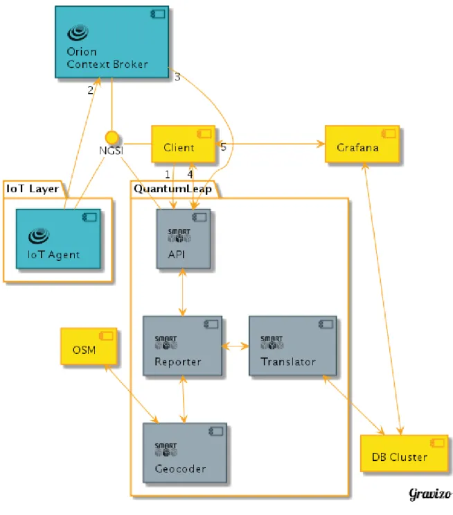
query records on both defined indices. Figure 3.2 shows a typical Quantum Leap setup. As shown, NGSI is the interface through which all components interact with each other.

Figure 3.2: Quantum Leap

When working with Quantum Leap, a client needs to set it up as a subscriber to the Orion Context Broker in order to be notified when a change occurs. Step 1 on the figure shows the client creating this subscription. After creating the subscription, Quantum Leap will be notified when the IoT agents in the IoT layer push any data to the Context Broker (Step 2) to which

3.2 NGSI-TSDB 18

Quantum Leap is subscribed and will receive this data (Step 3). The NGSI formatted data is received at the API endpoint and then passed on to the Reporter component. The Reporter analyzes the data, checks the syntax and parses it. If an address attribute is attached to the entity and geo-coding is enabled in the Quantum Leap configuration, the data is sent to the Geocoder component. The Geocoder processes the address attribute with the aid of geographical information obtained from OpenStreetMap and adds an attribute called location representing the geographical location of this address to the entity.

The Reporter then forwards the parsed and validated data to the Translator component. This component transforms the data into time series records, indexed by time and optionally by location as well. When this is done, the data is stored in a database cluster. It is not necessary however, to be limited to only one Translator. If there are different database systems, it is possible to set up a Translator component for each of them. The Reporter can then decide to which Translator to send the processed data, based on how it was configured.

Once Quantum Leap has processed and stored time series records, the client can start querying them. Data selectors to specify the data to be retrieved consist of temporal intervals, geographical areas and basic aggregate functions such as averages. To return queries, Quantum Leap will first convert the received web requests into SQL queries. Then it will extract the necessary time series data from the database cluster and utilize the Translator and Reporter components to turn the record data back into entities conforming to the NGSI interface and transmit them to the clients (Step 4).

The interactions shown in Step 5 in the diagram are to be added to Quantum Leap in the near future. The idea here is to forego the step of converting time series records back into NGSI entities. Visualization tools, such as Grafana should be able to directly query the database cluster when using Quantum Leap and render visualizations based on the time series data. Web clients can then use these visualizations directly.

3.2.2 Obelisk

As shortly mentioned in the introduction, Obelisk is a platform for building scalable applications on IoT centric timeseries data [2], developed by imec. To supply its data, Obelisk implemented an NGSI-TSDB interface, making it interoperable with other Smart City solutions using NGSI. The Obelisk API abstracts sensors and actuators that generate the data and provide them to clients as ”Things”. This abstraction is provided by DYAMAND.

3.3 NGSI-LD 19

DYAMAND (DYnamic, Adaptive MAnagement of Networks and Devices) is a middleware layer framework aimed at overcoming inter- and intra-domain interoperability issues that arise from using sensor interfaces of different types or vendors across different application domains [15]. Obelisk divides its different data sets into scopes. Scopes isolate data values so that developers of an application for company A cannot access the data of company B. Scopes can be limited and bounded through time periods, geographic areas, a list of only certain metrics and data tag expressions, which are custom tags to further filter data values.

The data generated by the Things in Obelisk belong to certain metrics, such as NO2 levels, air humidity, temperature and many more. Through these metrics, historical data belonging to this metric can be queried.

The query model allows for high granularity data selectors. Time intervals in milliseconds and spatial areas can be passed along as parameters with queries. These spatial areas are defined as geohashes.

Geohashing

Geohashing is a public domain algorithm created by Gustavo Niemeyer used to convert two-dimensional latitude, longitude pairs to strings of letters and numbers [16]. The algorithm divides the world into cells and each latitude, longitude pair indicates such a cell. The content and length of the hashed strings is based on the level of precision at which the algorithm operates. Figure 3.3 shows how the algorithm works. The world is alternately divided according to latitude and longitude. Each division adds a new level of precision. The image shows how the cells at each level are encoded into a binary string. This way, the world space can progressively be divided until the desired level of precision is reached. The resulting string is represented in base32 format.

3.3

NGSI-LD

The platforms described above provide an NGSI-TSDB interface for clients to interact with. However, this data is not yet linked data in any way. The NGSI-LD (NGSI-Linked Data) specification is an evolution of NGSIv2 and provides better support for linked data in the context of NGSI. NGSI-LD revolves around three concepts: entities, properties and relationships. Entities are similar to entities in NGSIv2 and are represented in JSON-LD. The reason for this is that JSON-LD supports representing JSON terms as URIs. Properties can be considered as

3.4 NGSI-LDF server 20

Figure 3.3: Geohashing division

a combination of an attribute and value and are attached to entities. Relationships are used to link entities to other related entities.

3.4

NGSI-LDF server

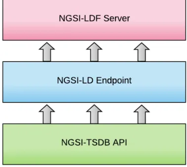
While NGSI-LD offers linked data support, it still has a few shortcomings. NGSI does not provide aggregation capabilities or historic data querying. The NGSI-LDF server developed by Harm Delva adds those capabilities and offers time series data as Linked Data Fragments [17]. Using Linked Data Fragments splits the time series data into pieces, classifying each element according to its measurement location and timestamp. Fragments are linked together through URIs so the data can be easily traversed. This decreases request specificity: clients no longer receive the exact data they requested. Instead, Linked Data Fragments containing the desired data are returned. Clients need to filter these fragments to extract the desired data. Linked Data Fragments can easily be cached and reused across multiple clients, decreasing the server cost. In order for the server to work, it needs an API endpoint that provides NGSI-LD (NGSI-Linked Data) compliant data. Both the NGSI-LDF server and the used NGSI-LD endpoint are Express-based servers and use the same type of air quality data as this thesis.

The process happens in two steps: first, the NGSI-LD endpoint is set up to query raw entity data from Obelisk. This data, which is formatted as JSON, is enhanced with context attributes. These context attributes are what turns the JSON data into Linked Data, which is called JSON-LD. They are used to map the properties in the JSON data to URLs. Through the context, an application may follow these links to find more related data. The setup is shown in figure 3.4. Note that this specific NGSI-LD endpoint is not a required component for the NGSI-LDF

3.4 NGSI-LDF server 21

Figure 3.4: NGSI-LDF Setup

server. The server can work with any NGSI-LD compliant endpoint.

Second, the data supplied by the NGSI-LD endpoint is fed to the NGSI-LDF server. This server then fragments the linked data documents in the geospatial dimension and in the temporal dimension.

3.4.1 Geospatial Fragmentation

In the geospatial dimension, fragmentation can happen in three ways. The first is through Slippy Map tiles. Contrary to the application developed for this thesis, these tiles do not have a fixed size and fragmentation can happen with multiple sizes. The size of a fragment is defined by the Slippy Map tile specification and uses an x-coordinate, y-coordinate and a zoom level z. The (x,y) coordinates indicate the location of the tile. The range of these coordinates is dependent on the zoom level, which indicates the distance from which the earth is observed. The higher the zoom level, the shorter this distance is and the more tiles are needed to represent the world and thus, the higher the range of values for x-coordinates and y-coordinates. Current supported zoom levels are 13 and 14. The second type of fragmentation is geohashing. This was already explained in section 3.2.2 so will not be discussed here again. The server supports geohashes with length 5 or 6. The final type of fragmentation is a hexagonal grid, called h3, a system

3.4 NGSI-LDF server 22

developed by Uber. The other two approaches use a more rectangonal grid as mapping. To identify tiles with this system, an index is required. Libraries such as h3-js can be used to find these indices.

3.4.2 Temporal Fragmentation

Fragmentation in the temporal dimension is fixed at one hour. This way, every fragment contains one hour of data belonging to one geospatial tile with measurements of all supported air quality metrics, timestamped at that particular hour and located in that specific tile.

3.4.3 Relation Between Fragments

To describe relations between fragments, the NGSI-LDF server makes use of the tree ontology. The tree ontology is a linked data vocabulary that can link different nodes, called tree:Nodes belonging to a hydra:Collection. It does this by describing parent-child relations between different tree:Nodes. These relations are defined by the tree:Relation entity and can be used to implement various comparisons between elements based on their values [18]. Figure 3.5 shows how this works in the context of the NGSI-LDF server.

3.4 NGSI-LDF server 23

Raw data fragments of the same tile are linked together through the tree:GreaterThanRelation and tree:LesserThanRelation relation entities and use the temporal fragmentation as ordering. What this means is, each fragment has a time interval of one hour, as stated earlier and contains an tree:GreaterThanRelation and an tree:LesserThanRelation attribute. The tree:GreaterThanRelation attribute has a link to the fragment that contains the data for the next hour. Same for the tree:LesserThanRelation attribute, but for the previous hour. This makes it possible for clients to navigate through time using these links and find all desired data. A tree:LesserThanRelation for the fragment that starts at 2019-11-25T16:00:00.000Z and ends at 2019-11-25T17:00:00.000Z is shown below.

"@type": "tree:LesserThanRelation", "tree:node": "http://localhost:3001/14/8393/5467?page=2019-11-25T15 ,→ :00:00.000Z", "sh:path": "ngsi-ld:observedAt", "tree:value": { "schema:startDate": "2019-11-25T15:00:00.000Z", "schema:endDate": "2019-11-25T16:00:00.000Z" }

There is a second type of link that exists on raw data fragments, one that connects them to the fragment containing the latest data. This relation attribute is called tree:AlternateViewRelation.

As can be seen on the figure, the server also supports server side summary fragments. The

way they are linked is the same as raw data fragments, with the addition of a tree:DerivedFromRelation, which points to the raw fragment - or fragments - from which the summary fragment is derived.

These summaries have a few more restrictions than the application developed for this thesis. It is for one, not possible to select a single aggregate metric. Instead, when querying summaries, all aggregate metrics are returned for the selected tile. The time interval over which these summary fragments span is also larger than for raw data fragments. Currently two aggregation intervals are available: hourly aggregations and daily aggregations. For the hourly aggregations, a period of six hours is calculated and returned. A whole week is returned for the daily aggregations. The aggregate metrics contained in these summary fragments are the standard deviation, sum, count, averages, minimum and maximum. In this aspect this implementation differs from the one developed for this thesis, where it is possible to select a specific aggregate function with

3.4 NGSI-LDF server 24

SOFTWARE IMPLEMENTATION 25

Chapter 4

Software Implementation

4.1

Data Model

The data used here is time series air quality data. So the data model needed to facilitate the modeling of sensors and sensor observations and do this compliant to linked data standards. The Semantic Sensor Network Ontology (SSN) was chosen, with its SOSA (Sensor, Observation, Sample, and Actuator) core ontology that contains the elementary classes and attributes. The data itself is represented in JSON-LD.

A fragment is made up of observations. These observations contain a measurement made by a sensor at a certain time and place. Below is an example of such an observation.

{ "@id":"http://example.org/data/airquality.no2.calib::number/lora ,→ .3432333855376318/1573315203092", "@type":"sosa:Observation", "hasSimpleResult":78.87322047543461, "resultTime":"2019-11-09T16:00:03.092Z", "observedProperty":"http://example.org/data/airquality.no2.calib::number", "madeBySensor":"http://example.org/data/lora.3432333855376318", "hasFeatureOfInterest":"http://example.org/data/AirQuality", "lat":51.238865023478866, "long":4.416282121092081 }

4.1 Data Model 26

Listing 4.1: Example of an observation in JSON-LD

It is also these observations that are aggregated into summaries. For this thesis, average and median were used as aggregate functions. Aggregate observations have the same format as above, minus the lat and long attributes and with the following properties added to them:

{ "usedProcedure":"http://example.org/data/id/average", "phenomenonTime":{ "rdf:type":"time:Interval", "time:hasBeginning":{ "rdf:type":"time:Instant", "time:inXSDDateTimeStamp":"2019-11-08T22:00:00.000Z" }, "time:hasEnd":{ "rdf:type":"time:Instant", "time:inXSDDateTimeStamp":"2019-11-08T23:00:00.000Z" } } }

Listing 4.2: Attributes belonging to an observation of a summary fragment

The reason for the lack of latitude and longitude is because summary observations are based on multiple raw observations and therefore cannot have an exact location. Instead the entire geospatial area in which the raw observations are located is considered as position of the summaries.

4.2 Architecture 27

4.2

Architecture

Figure 4.1: System Architecture

Figure 4.1 contains a diagram of the system architecture. Each component will be discussed.

4.2.1 Obelisk API

As already discussed in section 3, Obelisk provides raw sensor data. This API will be queried when the server receives an uncached HTTP request.

4.2.2 Server Side

The two LDF Server Nodes and the NGINX proxy each run in separate containers in a docker-compose setup.