Marian Schoorl | Anne Hollander |
Dik van de Meent
SimpleBox 4.0
A multimedia mass balance model for evaluating the fate of chemical substances
Colofon
© RIVM 2014
Parts of this publication may be reproduced, provided acknowledgement is given to: National Institute for Public Health and the Environment, along with the title and year of publication.
Marian Schoorl, Universiteit van Amsterdam Anne Hollander (author), RIVM
Dik van de Meent (author), RIVM
Contact:
Dik van de Meent DMG
dik.van.de.meent@rivm.nl
This investigation has been performed by order and for the account of I&M, within the framework of project REACH
This is a publication of:
National Institute for Public Health and the Environment
P.O. Box 1 | 3720 BA Bilthoven The Netherlands
Publiekssamenvatting
SimpleBox 4.0
SimpleBox is een van de rekenmodellen die het RIVM ontwikkelt voor het milieubeleid. Met dit model kan worden geschat aan welke
concentraties chemische stoffen mens en milieu blootstaan. SimpleBox wordt al twintig jaar gebruikt bij de ontwikkeling van Europese
regelgeving voor chemische stoffen (tegenwoordig: REACH-procedures) om te berekenen welke concentraties als veilig mogen worden
beschouwd. Het model is in 2014 geüpdatet op basis van de nieuwste wetenschappelijke inzichten en kan nu voor meer stoffen worden ingezet. Dit rapport bevat de gedetailleerde beschrijving voor technisch-wetenschappelijke onderzoekers en beleidsmakers.
Met SimpleBox kan de aanwezigheid van chemische stoffen in lucht, water en de bodem worden weergegeven. Het beschrijft ook hoe snel en in welke mate ze tussen deze compartimenten worden ‘uitgewisseld’. Stoffen in de lucht kunnen bijvoorbeeld door regen in de bodem terechtkomen.
De eerste versie van SimpleBox stamt uit 1986; de huidige versie 3.0, die momenteel in REACH dienst doet, is uitgebracht in 2004. Het vernieuwde model kan ook worden gebruikt voor stoffen die in het milieu geheel of gedeeltelijk als elektrisch geladen deeltjes (ionen) aanwezig zijn, zoals zware metalen en organische zuren en basen. Toekomstige modelvernieuwingen van SimpleBox zullen bovendien bruikbaar zijn voor nanomaterialen. Het RIVM ontwikkelt momenteel zo'n SimpleBox4nano in samenwerking met de Radboud Universiteit Nijmegen.
Het model wordt voor gebruik door onderzoekers en beleidsmakers beschikbaar gesteld via de RIVM-website www.rivm.nl/SimpleBox. Kernwoorden: milieumodellering, gifstoffen
Synopsis
SimpleBox 4.0
This document provides the technical description of the revised multi-media fate model SimpleBox 4.01 (20150331).
SimpleBox is a nested multi-media environmental fate model of the so-called Mackay level III/IV type. The environment is modelled as
consisting of well-mixed environmental compartments (air, water, sediment, soil, etc.), at three spatial scales. Emissions to the
compartments, transfer and partitioning between the compartments, and removal from the compartments are used to compute the steady-state and quasi-dynamic masses of chemical substance in the
environment. The SimpleBox model simulates the environmental fates of different substances in different landscape settings, of which the
characteristics are provided with the model database. In its default settings, SimpleBox returns results for a typical chemical, given a typical emission, to a typical environment.
SimpleBox vs. 4.01 (20150331) is an update of the SimpleBox vs 3.0 (20040614). Structural improvements made to the former version are the removal of the local scale and the vegetation compartments, and the addition of lake water and deep-sea water compartments. Further
improvements are a number of updates which implement new scientific insights in transport and degradation processes. The model’s application domain has been extended to cover a wider suite of chemical
substances, notably ionizing compounds such as metals, organic acids, and bases.
This report has been written to provide technical documentation for the new SimpleBox model.
Contents
Samenvatting — 9 1 Introduction — 11
1.1 Adjustments to the SimpleBox model — 11 1.2 Reader’s guide — 12
2 The SimpleBox model — 13 2.1 Model concept — 13
2.2 Scales and compartments — 13 2.3 Processes in SimpleBox — 13 3 Model calculations — 17 3.1 Model parameters — 17
3.2 Characteristics of the landscape — 22 3.3 Characteristics of the chemical — 23 3.3.1 Molecular weight — 23
3.3.2 Solid-water partitioning coefficient — 24 3.3.3 Gas-water partitioning coefficient — 25 3.3.4 Octanol-water partitioning coefficient — 26 3.3.5 pKa — 26
3.3.6 Fraction original species — 27 3.3.7 Vapour pressure — 27 3.3.8 Enthalpy of vaporization — 28 3.3.9 Solubility — 28 3.3.10 Enthalpy of dissolution — 28 3.3.11 Melting point — 28 3.3.12 Degradation rates — 28
3.4 Intermedia partitioning processes — 30 3.4.1 Air-water — 30 3.4.2 Aerosol solids-air — 31 3.4.3 Aerosol water-air — 32 3.4.4 Suspended solids-water — 32 3.4.5 Soil-water — 32 3.4.6 Sediment-water — 33
3.4.7 Colloidal organic matter-water — 34 3.5 Characteristics of the environment — 35 3.5.1 Air — 35 3.5.2 Water — 39 3.5.3 Sediment — 43 3.5.4 Soil — 44 3.6 Loss processes — 46 3.6.1 Degradation in air — 46 3.6.2 Degradation in water — 47 3.6.3 Degradation in sediment — 48 3.6.4 Degradation in soil — 49
3.7 Intermedia transfer processes — 50 3.7.1 Deposition — 50
3.7.2 Air to water and soil — 53 3.7.3 Water and soil to air — 56 3.7.4 Soil to water transfer — 58
3.7.6 Ocean mixing — 61
3.8 Mass balance equations-62 3.8.1 Air compartment-62 3.8.2 Water compartment-62 3.8.3 Sediment compartment-66 3.8.4 Soil compartment — 66 4 Model output — 69 4.1 Steady-state computation — 69 4.2 Quasi-dynamic computation — 73 5 The SimpleBox model code — 75 5.1 SimpleBox sheets — 75
5.1.1 Input — 75 5.1.2 Output — 75
5.1.3 Quasi-dynamic computation (“dynamicR”) — 75 5.1.4 Database — 77
5.1.5 Definition (“regional”, “continental” and “global”) — 77 5.1.6 Steady-state computation (“engine”) — 78
5.1.7 Operation — 78
5.2 Running the model — 79
6 References — 81
Samenvatting
Deze documentatie verstrekt de technische beschrijving van het
herziene multimedia lotgevallenmodel SimpleBox 4.01 (31 maart 2015). SimpleBox is een “genest” multimedia milieu lotgevallenmodel van het zogenaamde Mackay level III/IV-type. Het milieu wordt gemodelleerd als bestaande uit goed gemengde milieucompartimenten (lucht, water, sediment, bodem, et cetera) op drie ruimtelijke schalen. Emissies naar de compartimenten, transport en verdeling tussen de compartimenten, en verwijdering uit compartimenten worden gebruikt voor het berekenen van de steady-state en quasi-dynamische toestanden van milieuvervuiling, in termen van massa’s van stoffen in het milieu. SimpleBox simuleert het gedrag van verschillende chemische stoffen in verschillende milieus, waarvan de parameters in de met het model meegeleverde database zijn terug te vinden. Met alleen standaardwaarden modelleert SimpleBox de massa’s van een standaardstof in de compartimenten van een
standaardmilieu.
SimpleBox vs 4.01 (20150331) is een aangepaste versie van SimpleBox vs 3.0 (20040614). Structurele verbeteringen zijn de verwijdering van de lokale schaal en de vegetatiecompartimenten, en het toevoegen van een zoetwatermeer- en diepzeewatercompartimenten. Verder zijn nieuwe wetenschappelijke inzichten in transport en omzetting van stoffen in het nieuwe model geïmplementeerd. Hierdoor is het toepassingsgebied van het model uitgebreid en kunnen er meer
verschillende soorten stoffen worden gemodelleerd. Met name metalen en andere geheel of gedeeltelijk ionogene stoffen, zoals organische zuren en basen.
Dit rapport is bedoeld als technisch achtergronddocument voor het nieuwe SimpleBox model.
1
Introduction
A central issue in risk assessment of chemicals in the environment is the lack of information on the organisms’ levels of exposure to these
chemicals. In the late 1970s, the development of the first multimedia mass balance models (MMBM) provided an opportunity to predict the environmental fate of chemicals (Mackay, 1979). Thanks to these models, exposure levels of organisms to chemicals can now be
predicted, resulting in more powerful risk assessment and management. While the first models focused on screening and evaluation of the behaviour of chemicals, currently MMBMs are used to identify the behaviour of chemicals and data gaps, as well as to provide input for environmental policy and legislation. MMBMs are made up of multiple homogeneous compartments in a box; these can be at a local, regional, continental, or global scale. The concentration of a chemical in each homogeneous compartment such as air, water, soil or sediment is predicted using a separate equation. By combining all the
compartments’ equations, the model predicts the steady states and/or non-steady states of the chemicals.
SimpleBox is a nested multimedia environmental fate model in which the environmental compartments are represented by boxes. In the past few years some major changes have been made, resulting in a new version; SimpleBox 4.0. SimpleBox is a generic model; it can be customised to represent specific environmental situations. In its default setting, the SimpleBox computation represents the behaviour of a typical substance in a typical environment.
In 1982, the first SimpleBox was introduced at the RIVM; its complete history has been published by Brandes et al. (1996).
1.1 Adjustments to the SimpleBox model
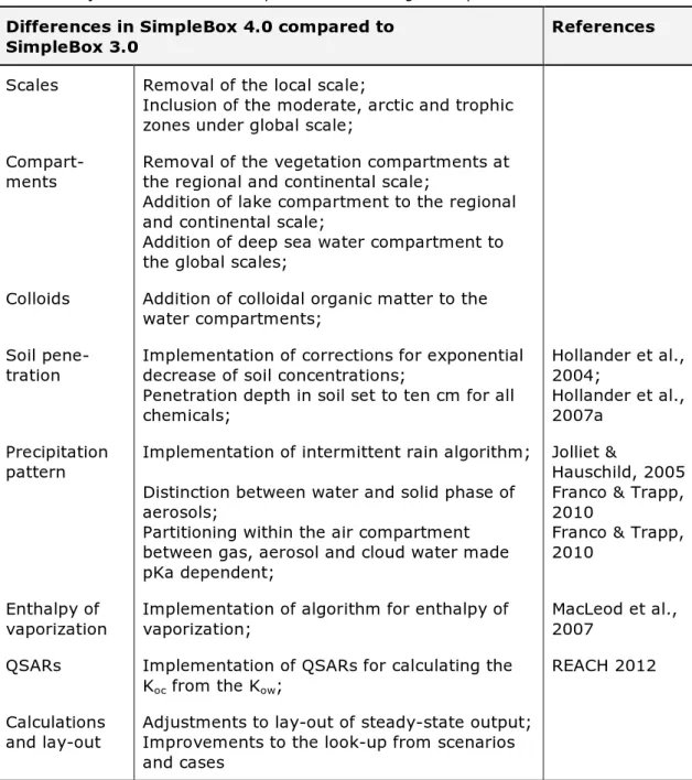
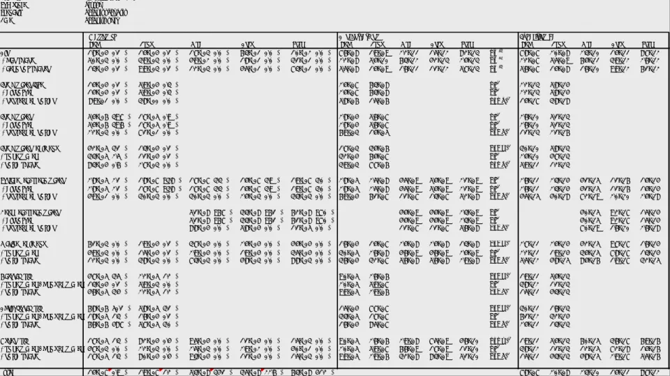
Both the transport processes between and the removal processes from all the compartments are described using equations. However, recent studies have shown that more accurate parameters or equations to describe certain processes are possible. An overview of all the improvements made to SimpleBox 4.0, are presented in Table 1. For example, the enthalpy of vaporization is set to a constant value in SimpleBox 3.0, while a relationship between this vaporization enthalpy and the subcooled liquid vapour pressure of a compound has been described (MacLeod et al., 2007). In addition, precipitation patterns are assumed to be continuous over the year. This results in a possible overestimation of removal of hydrophilic compounds due to wet
deposition (Jolliet & Hauschild, 2005). Franco & Trapp (2010) described new equations for more reliable predictions on ionized compounds. Therefore, the SimpleBox 3.0 model, which is only valid for neutral non-ionized compounds only, has been updated with routines for ionisable chemicals (Franco & Trapp, 2010), to obtain version 4.0. However, it is important to ensure that the partitioning of this class of chemicals depends on the pH of the compartment. As explained above, all
compartments are considered as being homogeneous, while an
exponential concentration profile in soils is described by Hollander et al., (2004, 2007a). To obtain more reliable and up-to-date predictions, all of these findings have been implemented in the SimpleBox model.
Table 1. Adjustments made to SimpleBox 3.0 resulting in SimpleBox 4.0. Differences in SimpleBox 4.0 compared to
SimpleBox 3.0 References
Scales Removal of the local scale;
Inclusion of the moderate, arctic and trophic zones under global scale;
Compart-ments Removal of the vegetation compartments at the regional and continental scale; Addition of lake compartment to the regional and continental scale;
Addition of deep sea water compartment to the global scales;
Colloids Addition of colloidal organic matter to the water compartments;
Soil pene-
tration Implementation of corrections for exponential decrease of soil concentrations; Penetration depth in soil set to ten cm for all chemicals; Hollander et al., 2004; Hollander et al., 2007a Precipitation
pattern Implementation of intermittent rain algorithm; Distinction between water and solid phase of aerosols;
Partitioning within the air compartment between gas, aerosol and cloud water made pKa dependent;
Jolliet &
Hauschild, 2005 Franco & Trapp, 2010
Franco & Trapp, 2010
Enthalpy of
vaporization Implementation of algorithm for enthalpy of vaporization; MacLeod et al., 2007 QSARs Implementation of QSARs for calculating the
Koc from the Kow;
REACH 2012
Calculations
and lay-out Adjustments to lay-out of steady-state output; Improvements to the look-up from scenarios and cases
1.2 Reader’s guide
This report is complementary to the technical documentation as described by Brandes et al. (1996). Chapter 2 describes the model concept and all the processes in the SimpleBox model, chapter 3
describes the improvements made to the model, chapter 4 describes the output possibilities of the model, and chapter 5 describes the SimpleBox model code.
2
The SimpleBox model
2.1 Model concept
SimpleBox (version 4) is an example of a level III and level IV “Mackay type” model, where both equilibrium steady-state and
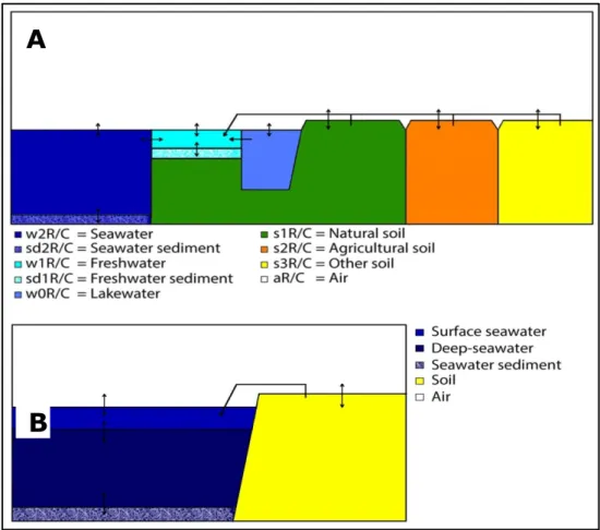
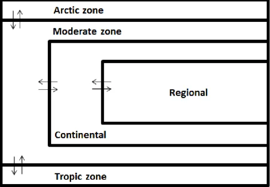
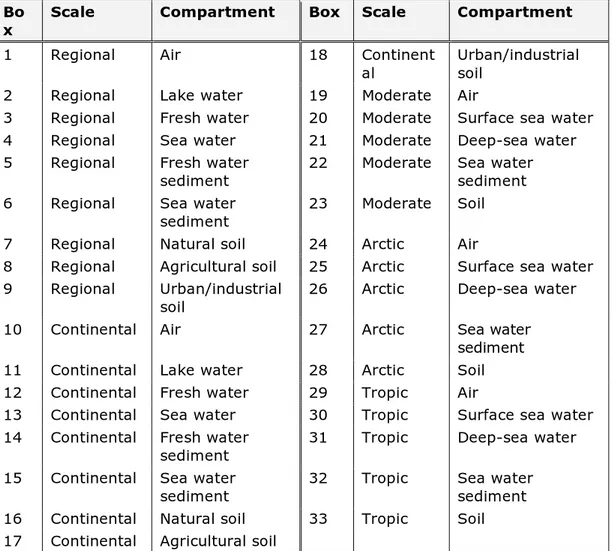
non-equilibrium non-steady-state are computed. This model contains a local scale containing eight compartments, regional and continental scales each containing nine compartments, and global zones, each containing five compartments (Figure 1; Hollander et al., 2007b).
Environmental compartments are represented by boxes. The mass of a chemical in these boxes is the result of various mass flow processes to and from the boxes. Entry mechanisms of chemicals into a box are: (a) emission (EMIS), (b) import flows of air or water (IMP) from boxes outside the spatial scale to which the box belongs, and (c) intermedia transport (IMT) from another box inside the spatial scale. Loss
mechanisms are: (d) degradation (DEG), (e) export (EXP) to outside the spatial scale, and (f) intermedia transport (IMT) to other boxes in the same spatial system. A mass balance equation can be written for each of the boxes. The mass balance equations have the following format: d𝑚𝑚��⃗𝑥𝑥(𝑡𝑡)
d𝑡𝑡 = 𝐸𝐸𝐸𝐸𝐸𝐸𝑆𝑆𝑥𝑥+ 𝐸𝐸𝐸𝐸𝑃𝑃𝑦𝑦→𝑥𝑥∙ 𝑚𝑚𝑦𝑦− 𝐸𝐸𝐸𝐸𝑃𝑃𝑥𝑥→𝑦𝑦∙ 𝑚𝑚𝑥𝑥+ 𝐸𝐸𝐸𝐸𝑇𝑇𝑧𝑧→𝑥𝑥∙ 𝑚𝑚𝑧𝑧− 𝐸𝐸𝐸𝐸𝑇𝑇𝑥𝑥→𝑧𝑧∙ 𝑚𝑚𝑥𝑥
− 𝐷𝐷𝐸𝐸𝐺𝐺𝑥𝑥∙ 𝑚𝑚𝑥𝑥
(1)
with
mx : mass of the chemical in box x [mol]
t : time [s]
EMISx : emission rate of the chemical into box x [mol∙s-1]
IMPy→x : import rate of the chemical from box y into box x [s-1]
EXPx→y : export rate of the chemical from box x into box y [s-1]
IMTz→x : intermedia transfer rate of the chemical from box z into box x [s-1]
IMTx→z : intermedia transfer rate of the chemical from box x into box z [s-1]
DEGx : loss rate of the chemical from box z [s-1]
2.2 Scales and compartments
SimpleBox 4.0 is a nested multimedia model consisting of three scales: regional, continental, and global. The global scale includes three zones: the arctic, moderate, and tropic. The regional and continental scales include nine compartments: air, lake water, freshwater, fresh water sediment, sea water, sea water sediment, natural soil, agricultural soil, and urban/industrial soil (Figure 1). At the global scale, each scale includes five compartments: air, surface sea water, deep-sea water, sea water sediment, and soil (Figure 1).
2.3 Processes in SimpleBox
Emissions can enter the air, water and soil compartments of all scales. Emission rates are expressed as products of production volumes and
Figure 1. Schematic view of the system and its compartments. A: Regional and continental scale, B: global scale.
emission factors, each of which needs to be entered by the modeller as model input.
Imports and exports of a substance enter and leave the air and water compartments of all spatial scales. At the regional and continental scales, fresh water flows through the lake water compartments via the fresh water compartments into the coastal marine and the ocean water compartments At the global scale, the water flows from tropical surface water through the moderate zone to the arctic zone and back through deep-sea waters. At all scales and global zones, air masses carry chemicals between air compartments. Import and export flow rates of water and air are considered constant in time. In addition, export of a substance occurs from the air compartments of all spatial scales by diffusion to the stratosphere.
Degradation of the substance occurs in all compartments at all scales. As with export with flowing air and water, and escape by diffusive transfer, degradation is a loss mechanism, assumed to obey (pseudo) first order kinetics. The first-order degradation rate constants
characterising the virtual degradation mass flows must be entered as input. Leaching of the substance occurs from the soil compartments into the groundwater, which is not considered to be part of the modelled system; leaching mass flows are considered as output terms. Unlike the
A
input mass flows, output mass flows are concentration dependent and become constant with time only when at steady state.
Intermedia transfer takes place between nearly all the compartments. Atmospheric deposition to soil and water in aerosol particles and rain droplets, run-off from soil to water, and leaching from soil are examples of advective transport. Gas absorption and volatilization across the air-soil and air-water interfaces are examples of diffusive transport.
Distinguishing between these types of transport is helpful because of the implications for the direction of the resulting (net) intermedia mass flows. Net transport between two compartments by diffusion can go both ways, depending on the concentrations of the chemical in the two adjacent media: diffusive transport from air to the earth’s surface is called gas absorption, diffusive transport in the opposite direction is called volatilization. As described by Brandes et al. (1996), diffusive intermedia transfer was successfully addressed by Mackay (2001) in his 'fugacity approach'. In the case of advective transport, a chemical is carried physically from one compartment into another so that the chemical mass flow strictly takes the direction of the carrier flow, independent of the (direction of) concentration gradients. Advective mass transfer can carry the chemical against the chemical potential or fugacity gradients.
3
Model calculations
In this chapter, the SimpleBox model is described in detail. In the following sections, the parameters and the equations for the landscape characteristics, chemical characteristics, partition coefficients,
degradation and transformation rates, intermedia partitioning and transfer processes are specified.
3.1 Model parameters
SimpleBox 4.0 contains multiple categories of parameters:
1. Default parameters: parameters that have a default value which is generally accepted or described in the literature (Table 2). 2. Input parameters: parameters that describe the substances or
landscape.
3. Calculated parameters: parameters that are described by a formula which contains other default, input and/or calculated parameters.
The following conventions are applied for symbols, where possible:
Parameters are mainly denoted in lower case (capitals indicating separate words), which indicate the type of the parameter.
Specification of the parameter and compartment for which the parameter is specified in subscript.
Specification of the scale is shown as a subscript in capital.
As an example, the symbol Fracaers,a[S] means the fraction (Frac) aerosol
solids (aers) in air (a) at a certain scale [S], denoted in the subscript ([S]); [S] may be the regional [R], continental [C], moderate [M], arctic [A] and tropic [T] scale.
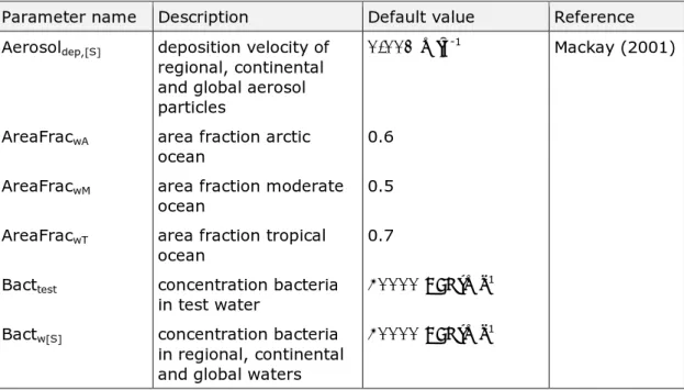
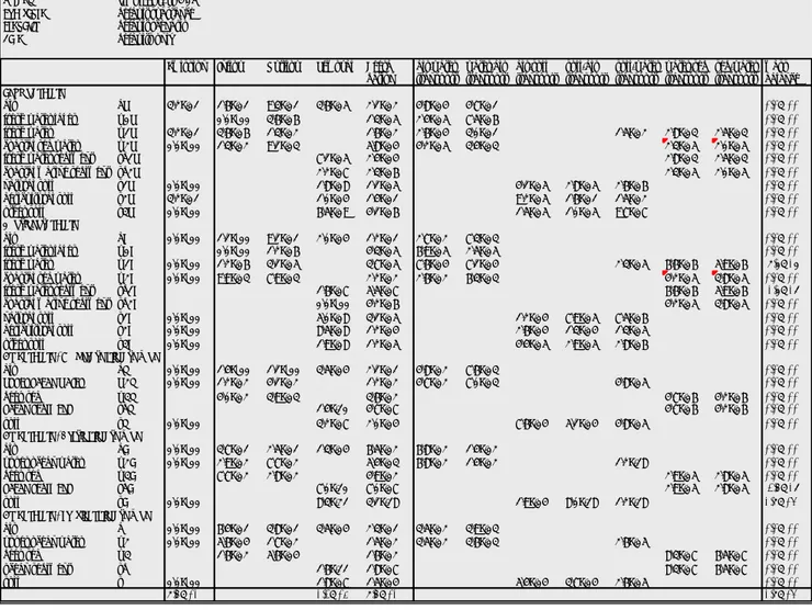
Table 2. Parameters with a default value used in the model.
Parameter name Description Default value Reference Aerosoldep,[S] deposition velocity of
regional, continental and global aerosol particles
0.001 m∙s-1 Mackay (2001)
AreaFracwA area fraction arctic
ocean 0.6
AreaFracwM area fraction moderate
ocean 0.5
AreaFracwT area fraction tropical
ocean 0.7
Bacttest concentration bacteria
in test water 40000 CFU∙ml
-1
Bactw[S] concentration bacteria
in regional, continental and global waters
Parameter name Description Default value Reference
COHrad,a[S] OH radical concentration 500000 cm-3 Den Hollander
et al., (2004) Collecteff[S] aerosol collection
efficiency representing the volume of air
efficiently scavenged by rain of its aerosol content, per unit volume of rain.
200000 Mackay (2001)
Colw[S] concentration of
colloidal organic matter in regional and
continental lake, fresh and sea water
0.001 kg∙m-3
Corg standard mass fraction organic carbon in soil/sediment
0.02 Den Hollander
& Van de Meent (2004)
Corgaers mass fraction organic
carbon in aerosol 0.1 Corgs[S] mass fraction organic
carbon in regional and continental natural and agricultural soil
0.02 Den Hollander
& Van de Meent (2004)
Corgsd[S] mass fraction organic
carbon in regional and continental lake, fresh and sea water sediment
0.05
Corgsusp[S] mass fraction organic
carbon in regional and continental lake, fresh and sea water
suspended matter
0.1
Depths[S] mixing depth regional,
continental and global soils
0.05 m for regional and continental natural land, other soils, and global soils; 0.2 m for the regional and continental agricultural soils Den Hollander & Van de Meent (2004)
Depthsd[S] mixed depth regional,
continental and global water sediments
Parameter name Description Default value Reference Depthw[S] mixed depth of regional,
continental and global sea waters
10 m for regional sea water;
200m for continental sea water;
100 m for global surface sea water; 3000 m for global deep sea water
EaOhrad Activation energy OH
radical reaction 6000 J∙mol
-1
Erosions[S] Erosion of global soils 0.000000000000951
m∙s-1
Fraca,s[S] volume fraction air in
regional, continental and global soils
0.2
Fracaers,a[S] Volume fraction solid
particles in regional, continental and global airs
0.00000000002
Fracaerw,a[S] Volume fraction
aqueous phase aerosols in regional, continental and global airs
0.00000000002
Fracinf,s[S] Volume fraction of
precipitation infiltrating into global soils
0.25
Fracrun,s[S] Volume fraction of
precipitation running off to global waters
0.25
Fracw,s[S] volume fraction water in
regional, continental and global soils
0.2
Fracw,sd[S] volume fraction water in
regional, continental and global sediments
0.8 Paterson & Mackay (1994)
H0sol enthalpy of dissolution described in
substance data,if not: 10000 J.mol-1
Heighta [S] mixed height of the
regional, continental and global air
1000 m Den Hollander & Van de Meent (2004)
k0OHrad frequency factor OH
Parameter name Description Default value Reference
Kp,col[S] colloidal organic
matter-water partitioning coefficient in global waters
220 L∙kg-1
kwsd,sed,sd[S] partial mass transfer
co-efficient for the sediment side of regional, continental and global water/sediment interface 0.00000002778 m.s-1 Mackay (2001)
kwsd,water,w[S] partial mass transfer
co-efficient for the water side of regional, continental and global water/sediment interface
0.000002778 m.s-1 Mackay (2001)
NetSed-Ratew[S] Net sediment
accumulation rate for regional, continental and global waters
0.0000000000868 m∙s-1 for regional fresh water; 0.0000000000862 m∙s-1 for continental fresh water; 0.0000000000634 m∙s-1 for regional sea
water; 0.0000000000274 m∙s-1 for continental sea water; 0.000000000000089 5 m∙s-1 for moderate sea water; 0.000000000000063 4 m∙s-1 for arctic/tropical sea water;
Ocean-Current global ocean circulation
current 150000000 m
3∙s-1
pHaerw pH aerosol water 3 Franco & Trapp
(2010)
pHcldw pH cloud water (average
of pH of water in air before oxidation (6.5) and after oxidation (4.7))
5.6 Franco & Trapp (2010)
pHs pH of soil 5 for natural soil;
7 for agricultural and other soil
Franco & Trapp (2010)
Parameter name Description Default value Reference pHw pH of water 7 for fresh water;
8 for sea water Franco & Trapp (2010)
Prodsusp,w[S] autochthonous
production of suspended matter in regional, continental and global waters
1.99 kg∙s-1 for
regional fresh water; 0.32 kg∙s-1 for
regional sea water; 32.39 kg∙s-1 for continental fresh water; 552.52 kg∙s-1 for continental sea water; 1229.88 kg∙s-1 for
moderate sea water; 808.6 kg∙s-1 for arctic
sea water; 2830.1 kg∙s-1 for
tropical sea water
Den Hollander & Van de Meent (2004)
Q10 rate increase factor per
10°C 2
RainRate[S] global annual
precipitation 2.22E-08 m∙s
-1 forthe
moderate scale; 4.12E-08 m∙s-1 for
the tropic scale; 7.93E-09 m∙s-1 for
the arctic scale Settl-Velocity[S] settling velocity of
suspended particles 0.0000289 m∙s -1 Den Hollander & Van de Meent, 2004 Suspw[S] concentration of suspended matter in regional and continental lake, fresh and sea water 0.0005 kg∙m-3 for lake water; 0.015 kg∙m-3 for fresh water; 0.005 kg∙m-3 for sea water Asselman (1997)
System-AreaA area arctic scale 42500000000000 m2
System-AreaT area tropical scale 127500000000000
m2
Temp[S] temperature global
scale 263 K for the arctic zone; 285 K for the moderate zone; 298 K for the tropical zone
Wind-Speed[S] average global wind
speed 3 m.s
Parameter name Description Default value Reference
ρaers dry density of aerosol
solids 2000 kg·m
-3
ρsolid mineral density of
sediment and soil 2500 kg·m
-3
3.2 Characteristics of the landscape
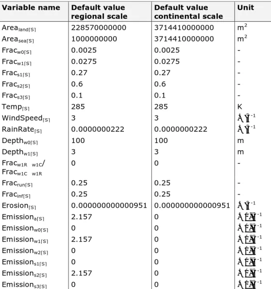
The landscape data in Table 3 contain values for the regional and continental landscape characteristics: area land and sea; fraction lake, fresh and sea water; fraction natural, agricultural and other soil; wind speed; rain rate; depth of lake and fresh water; river flow; fraction runoff; fraction infiltration; erosion and the emission scenario. In its default settings, SimpleBox represents the Earth’s northern hemisphere: continents surrounded by oceans in three climatic zones, and continents composed of river catchments, one of which is detailed as regional environment. In addition to this default landscape, specific landscapes can be selected from SimpleBox’s database, such as the standard EUSES landscape and 17 sub-continental landscapes, based on the REIMSEA model proposed by Wegener Sleeswijk et al. (2003).
Table 3. Default values for landscape characteristics. Variable name Default value
regional scale Default value continental scale Unit
Arealand[S] 228570000000 3714410000000 m2 Areasea[S] 1000000000 3714410000000 m2 Fracw0[S] 0.0025 0.0025 - Fracw1[S] 0.0275 0.0275 - Fracs1[S] 0.27 0.27 - Fracs2[S] 0.6 0.6 - Fracs3[S] 0.1 0.1 - Temp[S] 285 285 K WindSpeed[S] 3 3 m∙s-1 RainRate[S] 0.0000000222 0.0000000222 m∙s-1 Depthw0[S] 100 100 m Depthw1[S] 3 3 m Fracw1R→w1C/ Fracw1C→w1R 0 0 - Fracrun[S] 0.25 0.25 - Fracinf[S] 0.25 0.25 - Erosion[S] 0.000000000000951 0.000000000000951 m∙s-1
Emissiona[S] 2.157 0 mol∙s-1
Emissionw0[S] 0 0 mol∙s-1 Emissionw1[S] 2.157 0 mol∙s-1 Emissionw2[S] 0 0 mol∙s-1 Emissions1[S] 0 0 mol∙s-1 Emissions2[S] 2.157 0 mol∙s-1 Emissions3[S] 0 0 mol∙s-1
3.3 Characteristics of the chemical
The substance data describes the physical-chemical characteristics and degradation rates of 267 high production volume chemicals (HPVC; supporting information from Harbers et al., 2006). In SimpleBox 4.0, these characteristics are used for conversion of units, calculations of partitioning coefficients, and degradation of the substances. This section describes the physical-chemical characteristics used in the fate
calculation of SimpleBox 4.0.
3.3.1 Molecular weight
Molecular weight is used to calculate the gas and water diffusion coefficients and the partial mass transfer coefficients between air and water. In addition, molecular weight is used to convert the units of water solubility, emissions and output. If the molecular weight is not mentioned in the substance data, the median of all substances is used as default, 0.138 kilogram per mol.
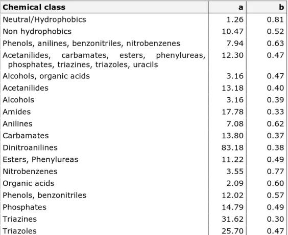
3.3.2 Solid-water partitioning coefficient
The solid-water partitioning coefficient is used to calculate the
partitioning coefficients of the suspended solids, sediment and soil to water and for estimating the degradation rate in sediment and soil. If the solid-water partitioning coefficient is not mentioned in the substance data, it can be obtained by means of QSARs (Franco & Trapp, 2008): For acids (original species):
𝐾𝐾𝑠𝑠𝑠𝑠= 100.54∙log 𝐾𝐾𝑜𝑜𝑜𝑜+1.11∙ 𝐶𝐶𝐶𝐶𝐶𝐶𝐶𝐶 ∙𝜌𝜌1000𝑠𝑠𝑠𝑠𝑠𝑠𝑠𝑠𝑠𝑠 (2)
For acids (alternate form):
𝐾𝐾𝑠𝑠𝑠𝑠,𝑎𝑎𝑠𝑠𝑎𝑎= 100.11∙log 𝐾𝐾𝑜𝑜𝑜𝑜+1.54∙ 𝐶𝐶𝐶𝐶𝐶𝐶𝐶𝐶 ∙𝜌𝜌1000𝑠𝑠𝑠𝑠𝑠𝑠𝑠𝑠𝑠𝑠 (3)
For bases (original species):
𝐾𝐾𝑠𝑠𝑠𝑠= 100.37∙log 𝐾𝐾𝑜𝑜𝑜𝑜+1.7∙ 𝐶𝐶𝐶𝐶𝐶𝐶𝐶𝐶 ∙𝜌𝜌1000𝑠𝑠𝑠𝑠𝑠𝑠𝑠𝑠𝑠𝑠 (4)
For bases (alternate form):
𝐾𝐾𝑠𝑠𝑠𝑠,𝑎𝑎𝑠𝑠𝑎𝑎= 10𝑝𝑝𝐾𝐾𝑎𝑎 0.65∙ 𝐾𝐾𝑜𝑜𝑜𝑜
1+𝐾𝐾𝑜𝑜𝑜𝑜 0.14
∙ 𝐶𝐶𝐶𝐶𝐶𝐶𝐶𝐶 ∙𝜌𝜌1000𝑠𝑠𝑠𝑠𝑠𝑠𝑠𝑠𝑠𝑠 (5)
For metals, solids-water partition coefficients need to be entered by users as model input. By default, a Kp value of 1000 is used:
𝐾𝐾𝑠𝑠𝑠𝑠= 1000 ∙ 𝐶𝐶𝐶𝐶𝐶𝐶𝐶𝐶 ∙𝜌𝜌1000𝑠𝑠𝑠𝑠𝑠𝑠𝑠𝑠𝑠𝑠 (6)
For other chemical classes:
𝐾𝐾𝑠𝑠𝑠𝑠= 𝑎𝑎 ∙ 𝐾𝐾𝑠𝑠𝑠𝑠𝑏𝑏∙ 𝐶𝐶𝐶𝐶𝐶𝐶𝐶𝐶 ∙𝜌𝜌1000𝑠𝑠𝑠𝑠𝑠𝑠𝑠𝑠𝑠𝑠 (7)
with
Ksw: dimensionless solids-water partitioning coefficient of the original
species [-]
Ksw,alt: dimensionless solids-water partitioning coefficient of the alternate
form [-]
Kow: octanol-water partitioning coefficient of the original species [-]
Corg: standard mass fraction organic carbon in soil/sediment [-]
ρsolid: mineral density in soil/sediment [kg∙m-3]
pKa: dissociation constant of (conjugated) acid [-]
1000: conversion factor [m3∙kg-1]
Where a and b values for the other chemical classes can be found in Table 4.
Table 4. Solid-water partitioning coefficient QSAR values for other chemical classes described by the European Commission (2003a).
Chemical class a b
Neutral/Hydrophobics 1.26 0.81
Non hydrophobics 10.47 0.52
Phenols, anilines, benzonitriles, nitrobenzenes 7.94 0.63 Acetanilides, carbamates, esters, phenylureas,
phosphates, triazines, triazoles, uracils 12.30 0.47
Alcohols, organic acids 3.16 0.47
Acetanilides 13.18 0.40 Alcohols 3.16 0.39 Amides 17.78 0.33 Anilines 7.08 0.62 Carbamates 13.80 0.37 Dinitroanilines 83.18 0.38 Esters, Phenylureas 11.22 0.49 Nitrobenzenes 3.55 0.77 Organic acids 2.09 0.60 Phenols, benzonitriles 12.02 0.57 Phosphates 14.79 0.49 Triazines 31.62 0.30 Triazoles 25.70 0.47
3.3.3 Gas-water partitioning coefficient
The air-water partitioning coefficient is used to calculate the scale specific air-water partitioning coefficient and the scale specific aerosol solids-water partitioning coefficient. If the air-water partitioning coefficient is not mentioned in the substance data, it can be obtained from: For 𝑃𝑃𝑣𝑣𝑎𝑎𝑝𝑝25> 100000: 𝐾𝐾aw= 100000 𝑆𝑆𝐶𝐶𝑆𝑆25 8.31 · 298 (8) For 𝑃𝑃𝑣𝑣𝑎𝑎𝑝𝑝25< 100000: 𝐾𝐾aw= 𝑃𝑃vap25 𝑆𝑆𝐶𝐶𝑆𝑆25 8.31 · 298 (9) with
Kaw: dimensionless gas-water partition coefficient of the original species [-]
Pvap25: vapour pressure of original species at 25°C [Pa]
Sol25: water solubility of original species at 25°C [mol·m-3]
8.31: gas constant [Pa∙m-3∙mol-1∙K-1]
298: temperature [K]
This estimation cannot be used for metals, and therefore the air-water partitioning coefficient is considered to be 1.0E-20.
3.3.4 Octanol-water partitioning coefficient
The octanol-water partitioning coefficient is used to estimate the water solubility, the apparent octanol-water partitioning coefficient, the organic carbon-water partitioning coefficient (original species and alternate form) and the aerosol solids-water partitioning coefficient. If no octanol-water partitioning coefficient is listed in the substance data, and the user does not specify one as model input, the median value of all substances in the database is used by default.
The octanol-water partitioning coefficient of the alternate form may be obtained from:
𝐾𝐾𝑠𝑠𝑠𝑠,𝑎𝑎𝑠𝑠𝑎𝑎= 10log 𝐾𝐾𝑜𝑜𝑜𝑜−3.5 (10)
with
Kow,alt: octanol-water partitioning coefficient of the alternate form [-]
Kow: octanol-water partitioning coefficient of the original species [-]
The apparent octanol-water partitioning coefficient is described by Trapp & Horobin (2005) and can be obtained from:
For acids: 𝐷𝐷 = �1 + 1017−𝑝𝑝𝐾𝐾𝑎𝑎� · 𝐾𝐾ow+ �1 − �1 + 1017−𝑝𝑝𝐾𝐾𝑎𝑎� · 𝐾𝐾ow,alt� (11) For bases: 𝐷𝐷 = �1 + 101𝑝𝑝𝐾𝐾𝑎𝑎−7� · 𝐾𝐾ow+ �1 − �1 + 101𝑝𝑝𝐾𝐾𝑎𝑎−7� · 𝐾𝐾ow,alt� (12) For neutrals: 𝐷𝐷 = 1 · 𝐾𝐾ow+ (1 − 1) · 𝐾𝐾ow,alt (13) with
D: apparent octanol/water partition coefficient at neutral pH [-]
pKa: dissociation constant of (conjugated) acid [-]
Kow: octanol/water partition coefficient of the original species [-]
Kow,alt: octanol/water partition coefficient of the alternate form [-]
7: neutral pH [-]
3.3.5 pKa
The dissociation constant of (conjugated) acid (pKa) is used to
determine the fraction of original species in waters, sediments and soils and to calculate the apparent octanol-water partitioning coefficient. For substances that may occur to a significant extent in their alternate (i.e. non-neutral) forms, it is essential that a pKa value is available. By default, a 50-50 split between original and alternate forms at neutral pH is assumed using a pKa value of 7.
3.3.6 Fraction original species
The fraction original species in aerosol water, in fresh water, in sea water, in sediments, in soils and in soil pore water are calculated in SimpleBox 4.0 in order to correct for ionisable compounds. These fraction original species for aerosol, fresh, sea and soil pore water can be determined using the Henderson-Hasselbalch equation (Henderson, 1908): For acids: 𝐹𝐹𝐶𝐶𝑠𝑠𝑜𝑜𝑠𝑠𝑜𝑜,𝑠𝑠 =1 + 101𝑝𝑝𝐻𝐻w−𝑝𝑝𝐾𝐾𝑎𝑎 (14) For bases: 𝐹𝐹𝐶𝐶𝑠𝑠𝑜𝑜𝑠𝑠𝑜𝑜,𝑠𝑠 =1 + 101𝑝𝑝𝐾𝐾𝑎𝑎−𝑝𝑝𝐻𝐻w For neutrals: 𝐹𝐹𝐶𝐶𝑠𝑠𝑜𝑜𝑠𝑠𝑜𝑜,𝑠𝑠 = 1 with
Frorig,w: fraction original species in aerosol, fresh, sea and soil pore
waters [-]
pHw: pH aerosol, fresh, sea and soil pore waters [-]
pKa: dissociation constant of (conjugated) acid [-]
The fraction original species in sediments and soil can be determined using equations proposed by Franco and Trapp (2008), which are derived from the Henderson-Hasselbalch equation (Henderson, 1908): For acids: 𝐹𝐹𝐶𝐶𝑠𝑠𝑜𝑜𝑠𝑠𝑜𝑜,𝑠𝑠/𝑠𝑠𝑠𝑠=1 + 10𝑝𝑝𝐻𝐻s/sd1 −0.6−𝑝𝑝𝐾𝐾𝑎𝑎 (15) For bases: 𝐹𝐹𝐶𝐶𝑠𝑠𝑜𝑜𝑠𝑠𝑜𝑜,𝑠𝑠/𝑠𝑠𝑠𝑠=1 + 101𝑝𝑝𝐾𝐾𝑎𝑎−4.5 (16) For neutrals: 𝐹𝐹𝐶𝐶𝑠𝑠𝑜𝑜𝑠𝑠𝑜𝑜,𝑠𝑠/𝑠𝑠𝑠𝑠= 1 (17) with
Frorig,s/sd: fraction original species in sediment and soil [-]
pHs/sd: pH sediment and soil [-]
pKa: dissociation constant of (conjugated) acid [-]
3.3.7 Vapour pressure
The vapour pressure is used to calculate Henry’s constant for both the original and the alternate form and the enthalpy of vaporization. If the vapour pressure is not mentioned in the substance data, the median of all substances is used as default; 4.7 Pascal.
3.3.8 Enthalpy of vaporization
The enthalpy of vaporization is used to calculate the scale specific air-water partitioning coefficients. The enthalpy of vaporization is substance dependent and is described by MacLeod et al. (2007):
With Tm>298: 𝐻𝐻0𝑣𝑣𝑎𝑎𝑝𝑝= �−3.82 ∙ 𝐿𝐿𝐿𝐿 �𝑃𝑃𝑣𝑣𝑎𝑎𝑝𝑝25∙ 𝑒𝑒−6.79∙�1− 𝑇𝑇 𝑚𝑚 298�� + 70� ∙ 1000 (18) With Tm≤298: 𝐻𝐻0𝑣𝑣𝑎𝑎𝑝𝑝= �−3.82 ∙ 𝐿𝐿𝐿𝐿�𝑃𝑃𝑣𝑣𝑎𝑎𝑝𝑝25� + 70� ∙ 1000 (19) with
H0vap: enthalpy of vaporization [J∙mol-1]
Pvap25: vapour pressure of original species at 25°C [Pa]
Tm: melting point [K]
298: temperature [K]
1000: conversion factor [J∙kJ-1]
3.3.9 Solubility
The solubility is used to calculate the Henry’s Law constant for both the original and the alternate form:
𝑆𝑆𝐶𝐶𝑆𝑆25= 10−1.214log 𝐾𝐾𝑜𝑜𝑜𝑜+0.85∙ 1000 (20)
with
Sol25: water solubility of neutral species at 25°C [mol∙m-3]
Kow: octanol-water partitioning coefficient of the original species
[mol∙L-1]
1000: conversion factor [dm3∙m-3]
3.3.10 Enthalpy of dissolution
The enthalpy of dissolution is used to calculate the scale specific air-water partitioning coefficient and has a default value of 10000 Joules per mol.
3.3.11 Melting point
The melting point of a substance is used to calculate the enthalpy of vaporization. If the melting point is not mentioned in the substance data, the median of all substances is used as default; 276 Kelvin.
3.3.12 Degradation rates
The degradation rates in air, water, sediment and soil are used to derive the scale specific removal rates in the air, water, sediment and soil compartments. If the degradation rate in air is not listed in the substance data, it can be obtained from (Wania & Daly, 2002):
𝑘𝑘𝑠𝑠𝑑𝑑𝑜𝑜,𝑎𝑎𝑠𝑠𝑜𝑜 = 𝐶𝐶𝑂𝑂𝐻𝐻𝑜𝑜𝑎𝑎𝑠𝑠,𝑎𝑎[𝑆𝑆]∙ 𝑘𝑘0𝑂𝑂𝐻𝐻𝑜𝑜𝑎𝑎𝑠𝑠∙ 𝑒𝑒
−𝐸𝐸𝑎𝑎𝑂𝑂𝑂𝑂𝑂𝑂𝑎𝑎𝑂𝑂
with
kdeg,air: gas phase degradation rate constant at 25°C [s-1]
COHrad,a[S]: OH radical concentration [cm-3]
k0OHrad: frequency factor OH radical reaction [cm3∙s-1]
EaOHrad: activation energy OH radical reaction [J∙mol-1]
8.314: gas constant [Pa∙m-3∙mol-1∙K-1]
298: temperature [K]
where the OH radical concentration, the frequency factor and the activation energy OH radical reaction are given in Table 2.
If degradation rate constants in water are not listed in the substance data, default half-lives for substances of which results from standard (OECD) tests are available can be used (European Commission, 2003a): For ready-biodegradable (r) substances:
𝑘𝑘𝑠𝑠𝑑𝑑𝑜𝑜,𝑠𝑠𝑎𝑎𝑎𝑎𝑑𝑑𝑜𝑜 = ln 2 15 ∙ 𝑄𝑄10 13 10 3600 ∙ 24 (22) with
kdeg,water: dissolved phase degradation rate constant at 25°C [s-1]
Q10: rate increase factor per 10°C [-]
where the rate increase factor per 10°C is given in Table 2.
For ready-biodegradable (r-) substances failing the ten-day window (see REACH TGD, European Commission 2003 a):
𝑘𝑘𝑠𝑠𝑑𝑑𝑜𝑜,𝑠𝑠𝑎𝑎𝑎𝑎𝑑𝑑𝑜𝑜 = ln 2 50 ∙ 𝑄𝑄10 13 10 3600 ∙ 24 (23) with
kdeg,water: dissolved phase degradation rate constant at 25°C [s-1]
Q10: rate increase factor per 10°C [-]
where the rate increase factor per 10°C is given in Table 2. For inherently biodegradable (i) substances:
𝑘𝑘𝑠𝑠𝑑𝑑𝑜𝑜,𝑠𝑠𝑎𝑎𝑎𝑎𝑑𝑑𝑜𝑜 = ln 2 150 ∙ 𝑄𝑄10 13 10 3600 ∙ 24 (24) with
kdeg,water: dissolved phase degradation rate constant at 25°C [s-1]
Q10: rate increase factor per 10°C [-]
where the rate increase factor per 10°C is given in Table 2.
For persistent (p) substances, the degradation rate in water is assumed to be 1.0E-20.
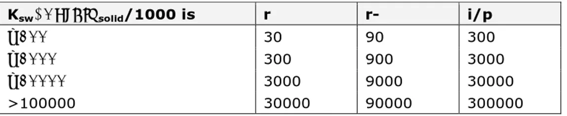
If the degradation rate in sediment is not mentioned in the substance data, it can be obtained from (European Commission, 2003a):
𝑘𝑘𝑠𝑠𝑑𝑑𝑜𝑜,𝑠𝑠𝑑𝑑𝑠𝑠 = 0.1 ∙ 𝑄𝑄10 13 10∙ ln (2) 𝑎𝑎 3600 ∙ 24 (25) with
kdeg,sed: bulk degradation rate constant standard sediment at 25°C [s-1]
Q10: rate increase factor per 10°C [-]
where the rate increase factor per 10°C is given in Table 2 and ‘a’ is derived from the biodegradation class and the partitioning from organic carbon in sediment to the water (Table 5).
Table 5. Half-lives (days) for sediment and soil based on biodegradation test results. Adapted from the European Commission (2003b).
Ksw/Corg∙ρsolid/1000 is r r- i/p
≤100 30 90 300
≤1000 300 900 3000
≤10000 3000 9000 30000
>100000 30000 90000 300000
If the degradation rate in soil is not mentioned in the substance data, it can be obtained from (European Commission, 2003a):
𝑘𝑘𝑠𝑠𝑑𝑑𝑜𝑜,𝑠𝑠𝑠𝑠𝑠𝑠𝑠𝑠 = 𝑄𝑄10 13 10∙ ln (2) 𝑎𝑎 3600 ∙ 24 (26) with
kdeg,sed: bulk degradation rate constant standard sediment at 25°C [s-1]
Q10: rate increase factor per 10°C [-]
where the rate increase factor per 10°C is given in Table 2 and ‘a’ in Table 5.
3.4 Intermedia partitioning processes
Intermedia equilibrium constants (air-water; aerosol-water; sediment-water; soil-water) or partition coefficients are required for various purposes, but principally for estimating intermedia mass transfer coefficients. The coefficients represent concentration ratios. Partition coefficients are available from experimental data or field measurements. More often, however, this information is not available. In these cases, the estimation methods described below can be used. It should be noted that, in general, the applicability of these estimation methods is limited to those classes of (organic) chemicals for which the relationships have been derived. Extrapolation beyond these limits may lead to errors of orders of magnitude.
3.4.1 Air-water
The air-water partition coefficient differs across the different scales of the SimpleBox model. The scale specific air-water partition coefficient can be obtained from:
𝐾𝐾𝑎𝑎𝑠𝑠[𝑆𝑆]= 𝐾𝐾𝑎𝑎𝑠𝑠∙ 𝑒𝑒 𝐻𝐻0𝑣𝑣𝑎𝑎𝑣𝑣
8.314 ∙�298−1 𝑇𝑇𝑑𝑑𝑇𝑇𝑝𝑝[𝑆𝑆]�1 ∙ 𝑒𝑒−𝐻𝐻08.314∙�𝑠𝑠𝑜𝑜𝑠𝑠 298−1 𝑇𝑇𝑑𝑑𝑇𝑇𝑝𝑝[𝑆𝑆]�1 ∙ 298
𝑇𝑇𝑒𝑒𝑚𝑚𝑇𝑇[𝑆𝑆] (27) with
Kaw[S]: dimensionless air-water partition coefficient of the original
species at regional, continental and global temperature [-]
Kaw: dimensionless gas-water partition coefficient of the original species [-]
H0vap: enthalpy of vaporization [J·mol-1]
Temp[S]: temperature [K]
H0sol: enthalpy of dissolution [J·mol-1]
8.31: gas constant [Pa∙m-3∙mol-1∙K-1]
298: temperature [K]
Where the dimensionless gas-water partition coefficient of the original species, the enthalpy of vaporization and the dissolution are described in Section 3.3.8; the regional and continental scale temperatures are described in Table 3; and the global scale temperature in Table 2.
3.4.2 Aerosol solids-air
The aerosol solids-water partitioning coefficient is calculated as
described by Harner & Bidleman (1998; adjusted according to Götz et
al., 2007): 𝐾𝐾𝑎𝑎𝑑𝑑𝑜𝑜𝑠𝑠,𝑎𝑎[S] = 0.54 ∙𝐾𝐾𝐾𝐾𝑠𝑠𝑠𝑠 𝑎𝑎𝑠𝑠∙ 𝐶𝐶𝐶𝐶𝐶𝐶𝐶𝐶𝑎𝑎𝑑𝑑𝑜𝑜𝑠𝑠∙ 𝜌𝜌𝑎𝑎𝑑𝑑𝑜𝑜𝑠𝑠 1000 (28) with
Kaers,a[S]: regional, continental and global dimensionless aerosol
solids-water partitioning coefficient [-]
Kow: octanol-water partitioning coefficient of the original species [-]
Kaw: dimensionless gas-water partitioning coefficient of the original
species at 25°C [-]
Corgaers: mass fraction organic carbon in aerosol [-]
ρaers: dry density of aerosol solids [kg∙m-3]
1000: conversion factor [m3∙kg-1]
Where the octanol-water partitioning coefficient and the gas-water partitioning coefficient are described in Sections 3.3.4 and 3.3.4, respectively. The mass fraction organic carbon in aerosol and the dry density of aerosol solids are described in Table 2.
3.4.3 Aerosol water-air
The aerosol water-water partitioning coefficient can be obtained from:
𝑘𝑘𝑎𝑎𝑑𝑑𝑜𝑜𝑠𝑠,𝑎𝑎[S]=𝐾𝐾 1
𝑎𝑎𝑠𝑠∙ 𝐹𝐹𝐶𝐶𝑠𝑠𝑜𝑜𝑠𝑠𝑜𝑜,𝑎𝑎𝑑𝑑𝑜𝑜𝑠𝑠 (29)
with
kaerw,a[S]: regional, continental and global dimensionless aerosol
water-water partitioning coefficient [-]
Kaw: dimensionless gas-water partitioning coefficient of the original
species at 25°C [-]
Frorig,aerw: fraction original species in aerosol water [-]
Where the gas-water partitioning coefficient and the fraction original species in aerosol water are described in Section 3.3.6.
3.4.4 Suspended solids-water
The suspended solids-water partitioning coefficient can be obtained from: 𝐾𝐾𝑝𝑝,𝑠𝑠𝑠𝑠𝑠𝑠𝑝𝑝[𝑆𝑆]= (𝐹𝐹𝐶𝐶𝑠𝑠𝑜𝑜𝑠𝑠𝑜𝑜,𝑠𝑠∙ 𝐾𝐾𝑠𝑠𝑠𝑠+ (1 − 𝐹𝐹𝐶𝐶𝑠𝑠𝑜𝑜𝑠𝑠𝑜𝑜,𝑠𝑠) ∙ 𝐾𝐾𝑠𝑠𝑠𝑠,𝑎𝑎𝑠𝑠𝑎𝑎) ∙ 1000 𝜌𝜌𝑠𝑠𝑠𝑠𝑠𝑠𝑠𝑠𝑠𝑠 𝐶𝐶𝐶𝐶𝐶𝐶𝐶𝐶 ∙ 𝐶𝐶𝐶𝐶𝐶𝐶𝐶𝐶𝑠𝑠𝑠𝑠𝑠𝑠𝑝𝑝[𝑆𝑆] (30) with
kp,susp[S]: regional, continental and global suspended solids-water
partitioning coefficient [-]
Frorig,w: fraction original species in water [-]
Ksw: dimensionless solids-water partitioning coefficient of the
original species [-]
Ksw,alt: dimensionless solids-water partitioning coefficient of the
alternate form [-]
Corg: standard mass fraction organic carbon in soil/sediment [-]
Corgsusp[S]: mass fraction organic carbon in regional, continental and
global suspended matter [-]
ρsolid: mineral density of soil/sediment [kg∙m-3]
1000: conversion factor [m3∙kg-1]
Where the fraction original species in water and the solids-water partitioning coefficients are described in Section 3.3.6 and 3.3.2, respectively. The standard mass fraction organic carbon in
soil/sediment, the mass fraction organic carbon in suspended matter, and the mineral density of soil/sediment are described in Table 2.
3.4.5 Soil-water
The soil-water partitioning coefficient may be derived from:
𝐾𝐾𝑝𝑝,𝑠𝑠[𝑆𝑆]= (𝐹𝐹𝐶𝐶𝑠𝑠𝑜𝑜𝑠𝑠𝑜𝑜,𝑠𝑠∙ 𝐾𝐾𝑠𝑠𝑠𝑠+ (1 − 𝐹𝐹𝐶𝐶𝑠𝑠𝑜𝑜𝑠𝑠𝑜𝑜,𝑠𝑠) ∙ 𝐾𝐾𝑠𝑠𝑠𝑠,𝑎𝑎𝑠𝑠𝑎𝑎) ∙
1000 𝜌𝜌𝑠𝑠𝑠𝑠𝑠𝑠𝑠𝑠𝑠𝑠
with
Kp,s[S]: regional, continental and global soil-water partitioning
coefficient [-]
Frorig,s: fraction original species in soil [-]
Ksw: dimensionless solids-water partitioning coefficient of the
original species [-]
Ksw,alt: dimensionless solids-water partitioning coefficient of the
alternate form [-]
Corg: standard mass fraction organic carbon in soil/sediment [-] Corgs[S]: mass fraction organic carbon in regional, continental and
global soil [-]
ρsolid: mineral density of soil/sediment [kg∙m-3]
1000: conversion factor [m3∙kg-1]
Where the fraction of original species in soil and the solids-water partitioning coefficients are described in Section 3.3.6. and 3.3.2, respectively. The standard mass fraction organic carbon in
soil/sediment, the mass fraction organic carbon in soil, and the mineral density of soil/sediment are described in Table 2.
The dimensionless soil-water partitioning coefficient can be derived from:
𝐾𝐾𝑠𝑠𝑠𝑠𝑠𝑠[𝑆𝑆]= 𝐹𝐹𝐶𝐶𝑎𝑎𝑐𝑐𝑎𝑎,𝑠𝑠[𝑆𝑆]∙ (𝐾𝐾𝑎𝑎𝑠𝑠[𝑆𝑆]∙ 𝐹𝐹𝐶𝐶𝑠𝑠𝑜𝑜𝑠𝑠𝑜𝑜,𝑠𝑠𝑠𝑠) + 𝐹𝐹𝐶𝐶𝑎𝑎𝑐𝑐𝑠𝑠,𝑠𝑠[𝑆𝑆]+ 𝐹𝐹𝐶𝐶𝑎𝑎𝑐𝑐𝑠𝑠,𝑠𝑠[𝑆𝑆]∙ 𝐾𝐾𝑝𝑝,𝑠𝑠[𝑆𝑆]∙𝜌𝜌1000𝑠𝑠𝑠𝑠𝑠𝑠𝑠𝑠𝑠𝑠 (32)
with
Kslw[S]: regional, continental and global dimensionless soil-water
partitioning coefficient [-]
Fraca,s: volume fraction air in regional, continental and global soil [-]
Kaw[S]: dimensionless air-water partitioning coefficient of the original
species at regional, continental and global temperature [-]
Frorig,sw: fraction original species in soil porewater [-]
Fracw,s[S]: volume fraction water in regional, continental and global soil
[-]
Fracs,s[S]: volume fraction solids in regional, continental and global soil
[-]
Kp,s[S]: regional, continental and global soil-water partitioning
coefficient [-]
ρsolid: mineral density of soil/sediment [kg∙m-3]
1000: conversion factor [m3∙kg-1]
Where the volume fraction air in soil, water in soil, and the mineral density of soil/sediment are described in Table 2. The volume fraction solid in soil is described in Equation 75. The fraction original species in soil pore water is described in Section 3.3.6. The air-water partitioning coefficient and the soil-water partitioning coefficient are described in Equation 27 and 31, respectively.
3.4.6 Sediment-water
𝐾𝐾𝑝𝑝,𝑠𝑠𝑠𝑠[𝑆𝑆] = (𝐹𝐹𝐶𝐶𝑠𝑠𝑜𝑜𝑠𝑠𝑜𝑜,𝑠𝑠𝑠𝑠∙ 𝐾𝐾𝑠𝑠𝑠𝑠+ (1 − 𝐹𝐹𝐶𝐶𝑠𝑠𝑜𝑜𝑠𝑠𝑜𝑜,𝑠𝑠𝑠𝑠) ∙ 𝐾𝐾𝑠𝑠𝑠𝑠,𝑎𝑎𝑠𝑠𝑎𝑎) ∙
1000 𝜌𝜌𝑠𝑠𝑠𝑠𝑠𝑠𝑠𝑠𝑠𝑠
𝐶𝐶𝐶𝐶𝐶𝐶𝐶𝐶 ∙ 𝐶𝐶𝐶𝐶𝐶𝐶𝐶𝐶𝑠𝑠𝑠𝑠[𝑆𝑆] (33) with
Kp,sd[S]: regional, continental and global sediment-water partitioning
coefficient [-]
Frorig,sd: fraction original species in sediment [-]
Ksw: dimensionless solids-water partitioning coefficient of the
original species [-]
Ksw,alt: dimensionless solids-water partitioning coefficient of the
alternate form [-]
Corg: standard mass fraction organic carbon in soil/sediment [-]
Corgsd[S]: mass fraction organic carbon in regional, continental and
global sediment [-]
ρsolid: mineral density of soil/sediment [kg∙m-3]
1000: conversion factor [m3∙kg-1]
Where the fraction original species in sediment and the solids-water partitioning coefficients are described in Section 3.3.6. and 3.3.2, respectively. The standard mass fraction organic carbon in
soil/sediment, the mass fraction organic carbon in soil, and the mineral density of soil/sediment are described in Table 2.
The dimensionless sediment-water partitioning coefficient can be derived from:
𝐾𝐾𝑠𝑠𝑠𝑠𝑠𝑠[𝑆𝑆]= 𝐹𝐹𝐶𝐶𝑎𝑎𝑐𝑐𝑠𝑠,𝑠𝑠𝑠𝑠[𝑆𝑆]+ 𝐹𝐹𝐶𝐶𝑎𝑎𝑐𝑐𝑠𝑠,𝑠𝑠𝑠𝑠[𝑆𝑆]∙ 𝐾𝐾𝑝𝑝,𝑠𝑠𝑠𝑠[𝑆𝑆]∙𝜌𝜌1000𝑠𝑠𝑠𝑠𝑠𝑠𝑠𝑠𝑠𝑠 (34)
with
Ksdw[S]: regional, continental and global dimensionless
sediment-water partitioning coefficient [-]
Fracw,sd[S]: volume fraction water in regional, continental and global
sediment [-]
Fracs,sd[S]: volume fraction solids in regional, continental and global
sediment [-]
Kp,sd[S]: regional, continental and global sediment-water partitioning
coefficient [-]
ρsolid: mineral density of soil/sediment [kg∙m-3]
1000: conversion factor [m3∙kg-1]
Where the volume fraction water in sediment and the mineral density of soil/sediment are described in Table 2. The volume fraction solids in sediment and the sediment-water partitioning coefficient are described in Equation 71 and 33, respectively.
3.4.7 Colloidal organic matter-water
The colloidal organic matter-water partitioning coefficient is described by Burkhard (2000) and can be obtained from:
with
Kp,col[S]: colloidal organic matter-water partitioning coefficient [-]
D: apparent octanol-water partitioning coefficient at neutral pH [-] Where the apparent octanol-water partitioning coefficient is described in Section 3.3.4.
3.5 Characteristics of the environment
The default settings for SimpleBox 4.0 are the Earth's northern
hemisphere with three climate zones ('moderate', 'arctic' and 'tropic'), one continental scale (within 'moderate') and one regional scale (within 'continental'). The regional system area can be obtained from:
𝑆𝑆𝑆𝑆𝑆𝑆𝑡𝑡𝑒𝑒𝑚𝑚𝑆𝑆𝐶𝐶𝑒𝑒𝑎𝑎𝑅𝑅= 𝑆𝑆𝐶𝐶𝑒𝑒𝑎𝑎𝑠𝑠𝑎𝑎𝑙𝑙𝑠𝑠,𝑅𝑅+ 𝑆𝑆𝐶𝐶𝑒𝑒𝑎𝑎𝑠𝑠𝑑𝑑𝑎𝑎,𝑅𝑅) (36)
with
SystemAreaR: regional system area [m2]
Arealand,R: area regional land [m2]
Areasea,R: area regional sea [m2]
Where the areas land and sea are described in Table 3.
The continental system area can be obtained from:
𝑆𝑆𝑆𝑆𝑆𝑆𝑡𝑡𝑒𝑒𝑚𝑚𝑆𝑆𝐶𝐶𝑒𝑒𝑎𝑎𝐶𝐶 = 𝑆𝑆𝐶𝐶𝑒𝑒𝑎𝑎𝑠𝑠𝑎𝑎𝑙𝑙𝑠𝑠,𝐶𝐶+ 𝑆𝑆𝐶𝐶𝑒𝑒𝑎𝑎𝑠𝑠𝑑𝑑𝑎𝑎,𝐶𝐶− 𝑆𝑆𝑆𝑆𝑆𝑆𝑡𝑡𝑒𝑒𝑚𝑚𝑆𝑆𝐶𝐶𝑒𝑒𝑎𝑎𝑅𝑅 (37)
with
SystemAreaC: continental system area [m2]
Arealand,C: area continental land [m2]
Areasea,C: area continental sea [m2]
SystemAreaR: regional system area [m2]
Where the areas land and sea are described in Table 3. The moderate system area can be obtained from:
𝑆𝑆𝑆𝑆𝑆𝑆𝑡𝑡𝑒𝑒𝑚𝑚𝑆𝑆𝐶𝐶𝑒𝑒𝑎𝑎𝑀𝑀= 85000000000000 − (𝑆𝑆𝑆𝑆𝑆𝑆𝑡𝑡𝑒𝑒𝑚𝑚𝑆𝑆𝐶𝐶𝑒𝑒𝑎𝑎𝐶𝐶+ 𝑆𝑆𝑆𝑆𝑆𝑆𝑡𝑡𝑒𝑒𝑚𝑚𝑆𝑆𝐶𝐶𝑒𝑒𝑎𝑎𝑅𝑅) (38)
with
SystemAreaM: moderate system area [m2]
8.5E13: area of the moderate zone [m2]
SystemAreaC: continental system area [m2]
SystemAreaR: regional system area [m2]
The arctic and the tropic system areas have default values, which can be found in Table 2.
3.5.1 Air
Air is treated in SimpleBox as a homogeneous compartment, consisting of a gas phase, an aerosol water phase, an aerosol solids phase, and a rain water phase; the concentration in air is a total concentration. The air in the system is not stagnant; it is continuously being flushed as wind blows air from a larger scale into the system, and from the system to a larger
scale. The wind blows from the regional scale, through the continental scale to the moderate zone and vice versa. From the moderate zone, the wind blows to the arctic and the tropical zones and vice versa. As the chemical is carried with these airstreams, this leads to "import" and "export" mass flows of the chemical to and from the system, see Figure 2. The refreshment rate is characterised by the atmospheric residence time.
Figure 2: Air flows between the scales in SimpleBox 4.0.
The volume of the air compartment in the urban, continental and global scales can be obtained from:
𝑉𝑉𝐶𝐶𝑆𝑆𝑉𝑉𝑚𝑚𝑒𝑒𝑎𝑎[𝑆𝑆]= 𝑆𝑆𝑆𝑆𝑆𝑆𝑡𝑡𝑒𝑒𝑚𝑚𝑆𝑆𝐶𝐶𝑒𝑒𝑎𝑎[𝑆𝑆]∙ 𝐻𝐻𝑒𝑒𝐻𝐻𝐶𝐶ℎ𝑡𝑡𝑎𝑎[𝑆𝑆] (39)
with
Volumea[S]: volume of the regional, continental and global air [m3]
SystemArea[S]: regional, continental and global system area [m2]
Heighta[S]: height of regional, continental and global air [m]
Where the height of the air compartment is described in Table 2.
The fraction of the chemical in the aerosol solids phase can be obtained from:
𝐹𝐹𝐶𝐶𝑎𝑎𝑑𝑑𝑜𝑜𝑠𝑠,𝑎𝑎[S]=1 + 𝐹𝐹𝐶𝐶𝑎𝑎𝑐𝑐 𝐹𝐹𝐶𝐶𝑎𝑎𝑐𝑐𝑎𝑎𝑑𝑑𝑜𝑜𝑠𝑠,𝑎𝑎[S]∙ 𝐾𝐾𝑎𝑎𝑑𝑑𝑜𝑜𝑠𝑠,𝑎𝑎[S]
𝑎𝑎𝑑𝑑𝑜𝑜𝑠𝑠,𝑎𝑎[S]∙ 𝐾𝐾𝑎𝑎𝑑𝑑𝑜𝑜𝑠𝑠,𝑎𝑎[S]+ 𝐹𝐹𝐶𝐶𝑎𝑎𝑐𝑐𝑎𝑎𝑑𝑑𝑜𝑜𝑠𝑠,𝑎𝑎[S]∙ 𝐾𝐾𝑎𝑎𝑑𝑑𝑜𝑜𝑠𝑠,𝑎𝑎[S] (40)
with
Fraers,a[S]: fraction of chemical in the aerosol solid phase [-]
Fracaers,a[S]: volume fraction solid particles in air [-]
Kaers,a[S]: dimensionless aerosol solid-air partitioning coefficient [-]
Kaerw,a[S]: dimensionless aerosol water-air partitioning coefficient [-]
Where the volume fraction solid particles in air and the volume fraction aqueous phase aerosols in air are described in Table 2. The dimensionless aerosol solid-air and aerosol water-air partitioning coefficients are
described in Equations 28 and 29, respectively.
The fraction of the chemical in the aerosol water phase can be obtained from:
𝐹𝐹𝐶𝐶𝑎𝑎𝑑𝑑𝑜𝑜𝑠𝑠,𝑎𝑎[S]=1 + 𝐹𝐹𝐶𝐶𝑎𝑎𝑐𝑐 𝐹𝐹𝐶𝐶𝑎𝑎𝑐𝑐𝑎𝑎𝑑𝑑𝑜𝑜𝑠𝑠,𝑎𝑎[S]∙ 𝐾𝐾𝑎𝑎𝑑𝑑𝑜𝑜𝑠𝑠,𝑎𝑎[S]
𝑎𝑎𝑑𝑑𝑜𝑜𝑠𝑠,𝑎𝑎[S]∙ 𝐾𝐾𝑎𝑎𝑑𝑑𝑜𝑜𝑠𝑠,𝑎𝑎[S]+ 𝐹𝐹𝐶𝐶𝑎𝑎𝑐𝑐𝑎𝑎𝑑𝑑𝑜𝑜𝑠𝑠,𝑎𝑎[S]∙ 𝐾𝐾𝑎𝑎𝑑𝑑𝑜𝑜𝑠𝑠,𝑎𝑎[S] (41)
with
Fraerw,a[S]: fraction of chemical in the aerosol water phase [-]
Fracaerw,a[S]: volume fraction aqueous phase aerosols in air [-]
Kaerw,a[S]: dimensionless aerosol water-air partitioning coefficient [-]
Fracaers,a[S]: volume fraction solid particles in air [-]
Kaers,a[S]: dimensionless aerosol solid-air partitioning coefficient [-]
Where the volume fraction solid particles in air and the volume fraction aqueous phase aerosols in air are described in Table 2. The
dimensionless aerosol solid-air and aerosol water-air partitioning coefficients are described in Equations 28 and 29, respectively. The fraction of the chemical in the gas phase can be obtained from:
𝐹𝐹𝐶𝐶𝑜𝑜𝑎𝑎𝑠𝑠,𝑎𝑎[S]= 1 − 𝐹𝐹𝐶𝐶𝑎𝑎𝑑𝑑𝑜𝑜𝑠𝑠,𝑎𝑎[S]− 𝐹𝐹𝐶𝐶𝑎𝑎𝑑𝑑𝑜𝑜𝑠𝑠,𝑎𝑎[S] (42)
with
Frgas,a[S]: fraction of chemical in the gas phase [-]
Fraerw,a[S]: fraction of chemical in the aerosol water phase [-]
Fraers,a[S]: fraction of chemical in the aerosol solids phase [-]
Air flows
Magnitudes of air flows are derived in SimpleBox from the residence times of air masses in air compartments. To estimate these residence times, it is assumed that air compartments are continuously refreshed by wind that blows at a constant speed of 3 ms-1 through a well-mixed
air box:
𝜏𝜏𝑎𝑎[𝑆𝑆]= 0.75 ∙�𝑆𝑆𝑆𝑆𝑆𝑆𝑡𝑡𝑒𝑒𝑚𝑚𝑆𝑆𝐶𝐶𝑒𝑒𝑎𝑎𝑊𝑊𝐻𝐻𝑊𝑊𝑊𝑊𝑆𝑆𝑇𝑇𝑒𝑒𝑒𝑒𝑊𝑊 [𝑆𝑆]
[𝑆𝑆] (43)
with
τa[S]: residence time in urban and continental air [s]
SystemArea[S]: regional, continental and global system area [m2]
WindSpeed[S]: regional, continental and global wind speed [ms-1]
0.75: empirical proportionality constant, according to Benarie (1980)
Where the regional and continental wind speeds are described in Table 3 and the global wind speed in Table 2.
The air flows from the regional scale to the continental scale and back, from the continental scale to the moderate zone and back, and from the moderate zone to the arctic and tropic zones and back. The airflows are obtained from:
𝑘𝑘𝑎𝑎𝑅𝑅→𝑎𝑎𝐶𝐶 =𝜏𝜏1
𝑎𝑎𝑅𝑅 (44)
with
kaR→aC:transfer rate of regional air to continental air [s-1]
τaR: residence time in regional air [s]
𝑘𝑘𝑎𝑎𝐶𝐶→𝑎𝑎𝑅𝑅 = 𝑘𝑘𝑎𝑎𝑅𝑅→𝑎𝑎𝐶𝐶∙𝑉𝑉𝐶𝐶𝑆𝑆𝑉𝑉𝑚𝑚𝑒𝑒𝑉𝑉𝐶𝐶𝑆𝑆𝑉𝑉𝑚𝑚𝑒𝑒𝑎𝑎𝑅𝑅
𝑎𝑎𝐶𝐶 (45)
with
kaC→aR: transfer rate of continental air to regional air [s-1]
kaR→aC: transfer rate of regional air to continental air [s-1]
VolumeaR: volume of the regional air [m3]
VolumeaC: volume of the continental air [m3]
Where the volumes of air compartments are described in Equation 39.
𝑘𝑘𝑎𝑎𝐶𝐶→𝑎𝑎𝑀𝑀=𝜏𝜏1
aC− 𝑘𝑘𝑎𝑎𝐶𝐶→𝑎𝑎𝑅𝑅 (46)
with
kaC→aM: transfer rate of continental air to moderate air [s-1]
τaC: residence time in continental air [s]
kaC→aR: transfer rate of continental air to regional air [s-1]
𝑘𝑘𝑎𝑎𝑀𝑀→𝑎𝑎𝐶𝐶= 𝑘𝑘𝑎𝑎𝐶𝐶→𝑎𝑎𝑀𝑀∙𝑉𝑉𝐶𝐶𝑆𝑆𝑉𝑉𝑚𝑚𝑒𝑒𝑉𝑉𝐶𝐶𝑆𝑆𝑉𝑉𝑚𝑚𝑒𝑒𝑎𝑎𝐶𝐶
𝑎𝑎𝑀𝑀 (47)
with
kaM→aC: transfer rate of moderate air to continental air [s-1]
kaC→aM: transfer rate of continental air to moderate air [s-1]
VolumeaC: volume of the continental air [m3]
VolumeaM: volume of the moderate air [m3]
Where the volumes of air compartments are described in Equation 39.
𝑘𝑘𝑎𝑎𝑎𝑎→𝑎𝑎𝑀𝑀 =𝜏𝜏1
𝑎𝑎𝑎𝑎 (48)
with
kaA→aM: transfer rate of arctic air to moderate air [s-1]
𝑘𝑘𝑎𝑎𝑀𝑀→𝑎𝑎𝑎𝑎 = 𝑘𝑘𝑎𝑎𝑎𝑎→𝑎𝑎𝑀𝑀∙𝑉𝑉𝐶𝐶𝑆𝑆𝑉𝑉𝑚𝑚𝑒𝑒𝑉𝑉𝐶𝐶𝑆𝑆𝑉𝑉𝑚𝑚𝑒𝑒𝑎𝑎𝑎𝑎
𝑎𝑎𝑀𝑀 (49)
with
kaM→aA: transfer rate of moderate air to arctic air [s-1]
kaA→aM: transfer rate of arctic air to moderate air [s-1]
VolumeaA: volume of the arctic air [m3]
VolumeaM: volume of the moderate air [m3]
Where the volumes of air compartments are described in Equation 39.
𝑘𝑘𝑎𝑎𝑇𝑇→𝑎𝑎𝑀𝑀=𝜏𝜏1
𝑎𝑎𝑇𝑇 (50)
with
kaT→aM: transfer rate of tropic air to moderate air [s-1]
τaT: residence time in tropic air [s]
𝑘𝑘𝑎𝑎𝑀𝑀→𝑎𝑎𝑇𝑇= 𝑘𝑘𝑎𝑎𝑇𝑇→𝑎𝑎𝑀𝑀∙𝑉𝑉𝐶𝐶𝑆𝑆𝑉𝑉𝑚𝑚𝑒𝑒𝑉𝑉𝐶𝐶𝑆𝑆𝑉𝑉𝑚𝑚𝑒𝑒𝑎𝑎𝑇𝑇
𝑎𝑎𝑀𝑀 (51)
with
kaM→aT: transfer rate of moderate air to tropic air [s-1]
kaT→aM: transfer rate of tropic air to moderate air [s-1]
VolumeaT: volume of the tropic air [m3]
VolumeaM: volume of the moderate air [m3]
Where the volumes of air compartments are described in Equation 39.
3.5.2 Water
At the regional and continental scale, three water compartments are present: lake water, fresh water and sea water. At the global scale, only sea water is present, which includes a surface sea water and a deep-sea water compartment. In SimpleBox, the water compartments are treated as homogeneous boxes, consisting of a suspended matter phase and a colloidal organic matter phase. The presence of suspended matter and colloidal organic matter influences the fate of chemicals in a very similar way to that of aerosol solids and aerosol water in the atmosphere. These phases bind the chemical, thus inhibiting it from taking part in the mass transfer and degradation processes that occur in the water phase. Suspended matter acts as a physical carrier of the chemical across the sediment-water interface. The colloidal organic matter only causes the chemical to be inhibited from taking part in mass transfer and
degradation processes. Concentration ratios among suspended matter, colloidal organic matter and water are often close to equilibrium. For multimedia fate modelling, the water compartment is treated the same way as the air, sediment and soil compartments: equilibrium is assumed among water, suspended matter and colloidal organic matter at all times. The water compartments at all scales are continuously flushed with water from outside that scale.