Fixed bed reactor design for calcium looping to capture CO2

(1)

capture CO2

Fixed bed reactor design for calcium looping to

Academic year 2019-2020

Master of Science in Chemical Engineering

Master's dissertation submitted in order to obtain the academic degree of

Counsellor: Varun Singh

Supervisors: Prof. dr. ir. Mark Saeys, Prof. dr. Vladimir Galvita

Student number: 01801088

Nilsu Bilgen

(2)

(3)

capture CO2

Fixed bed reactor design for calcium looping to

Master of Science in Chemical Engineering

Master's dissertation submitted in order to obtain the academic degree of

Counsellor: Varun Singh

Supervisors: Prof. dr. ir. Mark Saeys, Prof. dr. Vladimir Galvita

Nilsu Bilgen

(4)

ACKNOWLEDGMENTS

I would like to start by expressing my gratitude to my thesis promotors prof. dr. ir. Mark Saeys and prof. dr. Vladimir Galvita for giving me the opportunity to work on an inspiring project, for their guidance, and constructive feedback.

I would like to express my special thanks to my thesis counsellor Varun Singh for working diligently with me throughout this year, for his support, and valuable contributions.

I would also like to thank dr. Lukas Buelens for joining my thesis committee.

I sincerely thank assoc. prof. dr. Jean-François Portha for sharing his vision and expertise. I would also like to thank all the professors of the Department of Materials, Textiles and Chemical Engineering, who greatly contributed to my academic development and all of my classmates in the Chemical Engineering Program for sharing my master’s experience.

I sincerely thank the Government of Flanders for funding my master’s studies with the Master Mind Scholarship.

I would like to express my gratitude to my dear friends Oğuz Sarıgül and Mert Bayer for supporting me with their knowledge and advice.

Finally, I would like to give my special thanks to my family and friends, especially my husband Gerçek Armağan for his always smiling face, motivating words and endless enthusiasm. This accomplishment would not have been possible without their continuous encouragement.

(5)

LABORATORY FOR CHEMICAL TECHNOLOGY

Technologiepark 125, 9052 Gent, Belgium

Declaration concerning the accessibility of the master thesis

Undersigned, Nilsu Bilgen

Graduated from Ghent University, academic year 2019-2020 and is author of the master thesis with title:

Fixed Bed Reactor Design for Calcium Looping to Capture CO2

The author gives permission to make this master dissertation available for consultation and to copy parts of this master dissertation for personal use. In the case of any other use, the copyright terms have to be respected, in particular with regard to the obligation to state expressly the source when quoting results from this master dissertation.

31.05.2020 Nilsu Bilgen

(6)

Fixed Bed Reactor Design for Calcium Looping to Capture CO

2

Nilsu Bilgen

Supervisors: Prof. dr. ir. Mark Saeys, Prof. dr. Vladimir Galvita Counsellor: Varun Singh

Master's dissertation submitted in order to obtain the academic degree of Master of Science in Chemical Engineering

ABSTRACT

Due to the increase in energy demand and the necessity to mitigate the effects of greenhouse gas emissions, this study focuses on a promising novel technology for carbon capture, calcium looping. The main advantages of calcium looping are its reduced energy penalty and the use of a cheap and abundant CO2 sorbent. In this thesis, a multitubular fixed bed reactor is designed

to capture CO2 from an industrial flue gas stream. The mass and energy balances with kinetic

models for the carbonation and calcination reactions are solved by discretizing them spatially with the finite volume method. The resulting system of ordinary differential equations is solved using the ode15s solver in MATLAB. The rate of the carbonation reaction depends on the thermodynamic driving force, CaO conversion, and temperature through reaction kinetics. At higher temperatures the carbonation reaction occurs consecutively in each finite volume whereas at lower temperatures, it happens in more than one finite volume at a time. As the temperature increases, the cycle time and the operational cycle time also increase. To better incorporate the effect of the thermodynamic driving force, the force exerted from the previous finite volume is applied to the actual finite volume. The results demonstrate an increased rate of reaction. The non-isothermal and isobaric operation behaves similarly to the isothermal and isobaric operation due to the thickness and the internal diameter of the tubes, which enable the heat transfer to surroundings to be at the same order of magnitude with the reaction enthalpy. The experiments are designed to determine the reaction order, the reaction kinetics, and sorbent enhancement alternatives. They reveal that doping with supports, especially with Al, is beneficial in preserving the activity of the CaO sorbent.

KEYWORDS

(7)

Fixed Bed Reactor Design for Calcium Looping to

Capture CO

2

Nilsu Bilgen

Supervisors: Prof. dr. ir. Mark Saeys, Prof. dr. Vladimir Galvita Counsellor: Varun Singh

Abstract: Due to the increase in energy demand and the

necessity to mitigate the effects of greenhouse gas emissions, this study focuses on a promising novel technology for carbon capture, calcium looping. The main advantages of calcium looping are its reduced energy penalty and the use of a cheap and abundant CO2

sorbent. In this thesis, a multitubular fixed bed reactor is designed to capture CO2 from an industrial flue gas stream. The mass and

energy balances with kinetic models for the carbonation and calcination reactions are solved by discretizing them spatially with the finite volume method. The resulting system of ordinary differential equations is solved using the ode15s solver in MATLAB. The rate of the carbonation reaction depends on the thermodynamic driving force, CaO conversion, and temperature through reaction kinetics. At higher temperatures the carbonation reaction occurs consecutively in each finite volume whereas at lower temperatures, it happens in more than one finite volume at a time. As the temperature increases, the cycle time and the operational cycle time also increase. To better incorporate the effect of the thermodynamic driving force, the force exerted from the previous finite volume is applied to the actual finite volume. The results demonstrate an increased rate of reaction. The non-isothermal and isobaric operation behaves similarly to the isothermal and isobaric operation due to the thickness and the internal diameter of the tubes, which enable the heat transfer to surroundings to be at the same order of magnitude with the reaction enthalpy. The experiments are designed to determine the reaction order, the reaction kinetics, and sorbent enhancement alternatives. They reveal that doping with supports, especially with Al, is beneficial in preserving the activity of the CaO sorbent.

Keywords: power industry, carbon capture, calcium looping,

multitubular fixed bed reactor, CO2 sorbent

I. INTRODUCTION

The global energy demand continues to grow with the increase in population, growing prosperity especially due to emerging economies, and higher heating and cooling needs in certain parts of the world. With the increase in the use of fossil fuels as primary energy sources, global warming continues to be a concerning issue. The combustion of fossil fuels emits greenhouse gases, mainly CO2, which has been proven to be the primary reason for climate change.

Carbon capture and storage consists of the separation of CO2 from industrial and energy-related sources, transportation to a storage site, and long-term isolation from the atmosphere up to thousands of years [1]. In industrial applications, carbon capture and storage could decrease CO2 emissions by up to 4 gigatonnes per year by 2050, accounting for almost 9% of the reductions required to halve the energy-related emissions. In

by 2050. Power plants, oil refineries, natural gas processing, ammonia and ethylene oxide production, and cement, iron, and steel industries are the main industrial sources of CO2 emissions, so these are the most significant areas for potential applications of carbon capture technologies [2].

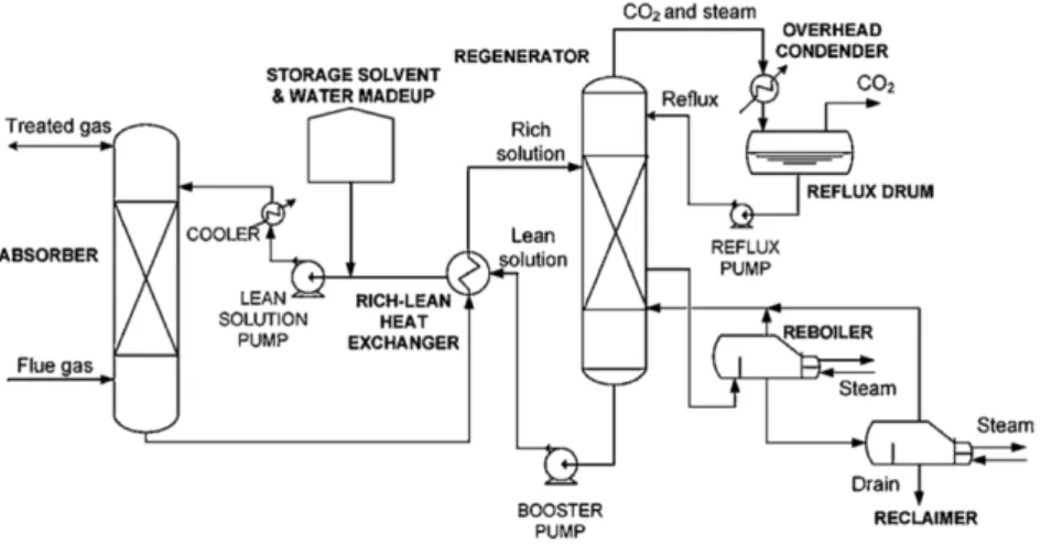
Calcium looping can be used to capture CO2 through pre and post-conversion as well as oxy-fuel combustion. It occurs through the continuous cycling of a CaO sorbent between two reactors. In one reactor, named as carbonator, CaO reacts with CO2 and removes it from the flue gas. The formed CaCO3 is fed to another reactor called calciner where the sorbent is regenerated. At the outlet of the calciner, the CaO is cycled back to the carbonator and a CO2-rich stream exits for storage and utilization [3]. The primary advantage of calcium looping is that it has a reduced energy penalty compared to other CO2 capture methods. The energy penalty is the reduction in the net efficiency of the power plant due to the energy requirements associated with CO2 capture and compression processes [4]. Romano [5] reports that for a CO2 capture efficiency of 80-90%, the energy penalty is 7-8% with respect to plants without a CO2 capture system and it is 1-5% energy penalty points advantaged over competitive oxyfuel plants. Markewitz et al. [6] state that for a coal-fired combustion process with an efficiency of 46%, the energy loss is 7.2% including the CO2 compression and processing. Other advantages of calcium looping are its synergy with heavy emitting industries such as cement production and steel manufacturing, and the use of a moderately cheap and abundant sorbent derived from natural limestone [7].

II. METHODOLOGY

Fixed bed reactors are investigated to be able to avoid sorbent losses, gas-solid separation, and attrition. Moreover, no prior studies focusing on calcium looping in fixed bed reactors are found in literature, so this study aims to investigate a potential alternative. Carbonation of CaO is a highly exothermic reaction; thus, heat management is a critical factor in designing a reactor for calcium looping. To increase the heat transfer surface area, a multitubular fixed bed reactor is chosen. The derived model equations of the fixed bed reactor design are discretized spatially with the finite volume method to yield a coupled ordinary differential equation (ODE) system and each element is treated as an ideally mixed control volume. An upwind scheme is used due to the defined flow direction. The resulting system of ODEs is solved with the ode15s solver in

(8)

one-dimensional models are chosen as a trade-off between model accuracy and complexity. The simulation algorithm is presented in Figure 1 and the equations mentioned will be explained in detail in the following sections.

Figure 1. The simulation algorithm A. Mass Balances

Time-dependent mass balances are written for gas and solid phases separately. The gas phase consists of CO2 and N2. The gas phase mass balance is based on equations derived by Wenzel et al. [8] and the evolution of the mole fraction of the gas component 𝛼 in the gas phase, 𝑥$(&), is described by,

()_*(+) (, = −𝜗0 ()_*(+) (1 + (3456) 5₆ 78 9_:,6𝜂=>>𝜈$ @A_B @, 3 C_B (1) 𝛼 = {𝐶𝑂G, 𝑁G} 𝛽 = {𝐶𝑎𝑂, 𝐶𝑎𝐶𝑂L}

The solid phase consists of CaO and CaCO3 and the evolution of the mole fraction of the solid component 𝛽 in the solid phase, 𝑥_M(N), is described as [8], ()_B(O) (, = 𝜂=>>𝜈M @A_B @, (2) B. Energy Balance

The energy balance is constructed to investigate the change in temperature with respect to time and distance, and to incorporate the temperature dependency of the kinetic constants and the equilibrium partial pressure of CO2. The energy balance is based on equations derived by Spallina et al. [9]. It consists of the convective heat transfer throughout the reactor, the axial heat dispersion, the reaction enthalpy, and the heat transfer to surroundings. The following assumptions are made: both gas and mass phases have the same temperature and the reaction enthalpies, the specific heats, the densities, and the heat transfer coefficients are constant. The evolution of

C. Kinetic Models

Calcium looping consists of two consecutive reactions which are carbonation and calcination.

1) Carbonation

The carbonation reaction is an exothermic, gas-solid reaction as follows,

𝐶𝑎𝑂(T)+ 𝐶𝑂G₍₆₎ → 𝐶𝑎𝐶𝑂L₍₈₎, ∆𝐻NVe= −180 𝑘𝐽/𝑚𝑜𝑙 (4)

The heterogeneous carbonation reaction occurs through two sequential stages. The initial fast stage is controlled by surface chemical kinetics. The driving force is the difference between the bulk partial pressure of CO2 and the equilibrium partial pressure of CO2. The formation and growth of CaCO3 is considered to be an important rate-limiting step during carbonation. As the CaCO3 starts to form and grow on the outer region of the CaO particle, it starts to prevent the contact between the unreacted core and the reacting gas. Due to this effect, the slower diffusion-controlled stage begins which is controlled by the diffusion of gas through the product layer of CaCO3 [10]. In most industrial applications, the diffusion-controlled stage is neglected because it is much slower [11].

In this study, the grain model is used to model the reaction kinetics of carbonation. The grain model focuses on how the grain size distribution changes over the course of the reaction and assumes that the material is made up of non-porous solid grains of CaO, randomly located in the particle and dispersed in the gas which is considered as the continuous phase [9].

Sun et al. [12] expresses the specific rate under kinetic control as,

@Aopq

@, (34Aopq)= 𝑀sXt𝑘9Xuv(𝑃stx− 𝑃stx,=y)

z_𝑆 ₍₅₎

The investigation of Sun et al. [12] shows that when the thermodynamic driving force, 𝑃stx− 𝑃stx,=y, is higher than 10 kPa, the reaction is zeroth order and when it is less than 10 kPa, the reaction is first order. The calculated kinetic parameters for limestone are shown in Table 1.

Table 1. Kinetic parameters by Sun et al. [12]

𝑷𝑪𝑶𝟐− 𝑷𝑪𝑶𝟐,𝒆𝒒 𝒏 𝒌𝟎 E

> 10 kPa 0 1.67x10-3 _mol/m2_/s _{29 ± 4 kJ/mol}

≤ 10 kPa 1 1.67x10-7 _mol/m2_/s/Pa _{29 ± 4 kJ/mol} 2) Calcination

The calcination reaction is an endothermic, gas-solid reaction as follows,

𝐶𝑎𝐶𝑂L₍₈₎→ 𝐶𝑎𝑂(T)+ 𝐶𝑂G₍₆₎, ∆𝐻NVe= 180 𝑘𝐽/𝑚𝑜𝑙 (6)

The calcination reaction is modeled based on the study conducted by Martinez et al. [13], which proposes using the shrinking core model due to its simplicity and ability to adequately model the reaction. The shrinking core model is derived from the homogenous particle model and the particle is defined as a non-porous sphere. This model discriminates between the product layer diffusion and reaction at the surface

(9)

Martinez et al. [13] calculate the necessary kinetic constants as 2.05x103_m3_{/mol/s for the pre-exponential factor, 𝑘}

Š, and

112 kJ/mol for the activation energy, 𝐸.

III. EXPERIMENTAL INVESTIGATION

The experimental investigation is planned to determine the reaction order and the kinetic parameters for the carbonation reaction, and to examine the effect of sorbent enhancement on deactivation trends. The intraparticle and transport resistances may lead to a kinetic analysis resulting with effective values instead of intrinsic properties [10]. In designing the set of experiments, the Eurokin spreadsheet for the assessment of transport limitations in gas-solid fixed bed reactors is used to consider these effects. It requires the physical properties of the components as well as operating conditions to determine the heat and mass transfer limitations.

In designing the experiments, the following phenomena are checked:

1. Relative pressure drop over the fixed bed using the Ergun equation [14]

2. Assumption of ideal plug flow behavior using the criterion proposed by Mears [14] and Gierman [15] 3. External mass transfer limitation using the Carberry

number [15]

4. Internal diffusion limitation using the Weisz-Prater criterion [17]

5. External heat transfer limitation using the criterion proposed by Mears [15]

6. Radial heat transfer limitation using the criterion proposed by Mears [15]

7. Adiabatic temperature rise

As a result of the preceding criteria, the following decisions for the experimental investigation are made:

• The total molar inlet flow rate of the feed gas is 0.09 mmol/s.

• The feed gas consists of 15% CO2 and 85% He. • The solid phase consists of CaO and SiC which is used

as the diluent. The mass ratio of CaO over SiC is 0.1 • To be in the first order region of carbonation, the

difference between the partial pressure of CO2 and equilibrium partial pressure of CO2 should be below 10 kPa, so the temperatures and pressures are chosen accordingly.

The following experiments mentioned in sections IIIA and IIIB were not conducted due to Covid-19 measures; thus, these sections aim to give guidelines for further research.

A. Determination of the Reaction Order

Using the grain model [18] and the specific rate under kinetic control [12] the following equation is derived,

𝑙𝑛𝑟Š= ln •Copq_L‘’p“”• + 𝑛𝑙𝑛P𝑃stx− 𝑃stx.=yU + 𝑙𝑛𝑆Š (8) The slope of the 𝑙𝑛𝑟Š vs 𝑙𝑛P𝑃stx− 𝑃stx.=yU plot gives the order of the carbonation reaction with respect to the partial pressure of CO2. In order to determine the reaction order, experiments shown in Table 2 will be conducted. By varying the partial pressure of CO2, the dependence of carbonation reaction rate on the partial pressure of CO2 will be investigated.

Table 2. Experiments for the determination of the reaction order

Experiment

number Temperature (K)

Partial pressure of

CO2 (kPa) Time (min)

1 973 13 30

2 973 15 30

3 973 17 30

4 973 19 30

B. Determination of the Kinetic Parameters

Using the Arrhenius relation, the reaction rate constant can be expressed as,

𝑘 = 𝑘Šexp •4š_\V• (9)

Thus, Equation 8 can be rewritten as,

𝑙𝑛𝑟Š= ln •Copq_L‘›N›• −_\Vš (10)

By linearly fitting Equation 10 with the experimental data, the activation energy 𝐸 and pre-exponential factor 𝑘Š will be

determined. In order to determine the kinetic parameters, experiments shown in Table 3 will be conducted. By varying the operating temperature, the activation energy and the pre-exponential factor will be investigated.

Table 3. Experiments for the determination of kinetic parameters

Experiment

number Temperature (K)

Partial pressure of

CO2 (kPa) Time (min)

1 773 15 30

2 823 15 30

3 873 15 30

4 923 15 30

C. Sorbent Enhancement

Sorbent deactivation is an important phenomenon that greatly affects carbon capture performance. Since in fixed bed reactors it is operationally difficult to replace the sorbent, enhancing sorbent activity is an important aspect in design. In this study, different inert support materials, namely Al, Ce, and Mg are investigated to determine their effects on the activity of the CaO sorbent.

The experimental specifications are as follows:

The sample mass is 100 mg composed of 83 mass% CaO and the rest is inert support material under investigation. The particle size of the sorbent is in the 355 and 500 μm range. The total flow rate is 2.7 mmol/min. The instrument used for conducting the experiments is Micromeritics Autochem II 2920.

The experimental procedure is as follows:

The experiments are conducted under ambient pressure. Carbonation occurs at 923 K by flowing gas with 15 vol% CO2 and the rest being He for 10 minutes. After carbonation, the temperature is ramped from 923 to 1233 K at 10 K/min in a flow of 90 vol% CO2 in He. Once 1233 K is reached, calcination is continued under a flow of 90 vol% CO2 in He for 15 minutes and then the gas flow is switched to He which continues for another 15 minutes. This procedure is repeated for 10 cycles.

(10)

IV. RESULTS AND DISCUSSION

A. Simulation Results for the Carbonator Reactor Design The design of the carbonator consists of a multitubular fixed bed reactor made up of 2000 tubes with a length of 15 m and a diameter of 0.045 m. Each tube is discretized into five finite volumes with a height of 3 m and each volume is treated as a continuously stirred tank reactor. The composition of the feed gas of the carbonator is 15 vol% CO2 and 85 vol% N2, which is close to the typical flue gas composition of refineries and coal-fired power plants. The feed gas is assumed to be free of impurities such as SOx, NOx, and water. The initial conditions in the reactor are chosen as pure N2 in the gas phase and 100 mass% CaO sorbent in the solid phase. The carbonator reactor design aims to capture 90 vol% from the feed gas stream and in order to achieve this, the molar fraction of CO2 in the outlet gas should be below 1.5 vol%. The capacity of the process is determined as 1 t/h CO2, hence the superficial velocity of the gas phase is calculated as 1.1 m/s.

1) Isothermal and Isobaric Operation

Simulation results for the isothermal and isobaric operation at 873 K and ambient pressure are shown in Figure 2.

Figure 2. The simulation results for isothermal and isobaric operation at 873 K and ambient pressure. a) Temperature (K) with respect to time (h) b) Rate of reaction (1/s) with respect to time (h) c) Thermodynamic driving force (Pa) with respect to time (h) d) Mole fraction of CO2 (-) with respect to time (h) e) Mole fraction of CaO (-) with respect to time (h) f) Mole fraction of CaCO (-) with respect

equilibrium partial pressure of the CO2 at the operating temperature. Since it is never below zero, the calcination reaction is not favored.

Once the feed gas consisting of 15 vol% CO2 is fed to the reactor; the CO2 instantaneously starts to react with the CaO in the first finite volume. Thus, the mole fraction of CO2 is lowered down to 0.0027 which is its equilibrium value at 873 K. The mole fraction of CO2 cannot be below this value because the reaction is equilibrium limited. After 26 h, the mole fraction of CO2 starts to increase because the CaO available for the carbonation reaction is below 20 mol% from this point on.

Between 0 and 33 h, the mole fraction of CO2 remains below 0.11 in the first finite volume, resulting in the thermodynamic driving force being lower than 10 kPa. When the thermodynamic driving force is lower than 10 kPa, the reaction is modeled as first order. The rate of the first order carbonation reaction depends on the thermodynamic driving force, CaO conversion, and temperature through reaction kinetics. In isothermal operation, the temperature remains constant at 873 K, therefore the reaction kinetics, namely the first order rate constant, also remains constant at 3.1x10-9_mol/m2_/Pa/s throughout the isothermal operation. Secondly, since the thermodynamic driving force is a function of the partial pressure of CO2, it is relatively lower between 0 to 26 h and starts to increase significantly from thereon. Lastly, as conversion increases, the reaction rate decreases. The evolution of conversion can be tracked from the decrease in the mole fraction of CaO and the increase in the mole fraction of CaCO3. As a result of the above mentioned three components, the reaction rate is calculated as 4.9x10-2_{1/s at the initial conditions} of 15 vol% CO2 and 100 mass% CaO. As CO2 enters the reactor, its mole fraction instantaneously decreases, which significantly reduces the thermodynamic driving force, leading to lower reaction rates around 8.5x10-6_{1/s. The rate of reaction} fluctuates around this value for 33 h in the first finite volume. The reaction rate starts to slow down reaching 0 1/s at 35 h because of the full conversion of CaO. At this point, all CaO in the first finite volume is depleted so the output of this finite volume becomes 15 vol% CO2 in the gas phase.

The reaction almost occurs in consecutive stages in each finite volume. This behavior is investigated by comparing the reaction time and the residence time. The residence time is calculated by dividing the length of the finite volume by the velocity of the gas phase and found to be 2 s. The reaction time is calculated from the second term on the right-hand side of the gas phase mass balance (Equation 1) and found to be 0.06 s, initially for the first finite volume. Since the residence time is longer than the reaction time, CO2 reacts in the first finite volume without being transferred to the next finite volume. As the reaction proceeds, its rate decreases, increasing the reaction time. At 33 h, the reaction time becomes longer than the residence time, therefore a part of the CO2 stream is transferred to the next finite volume. The CO2 mole fraction of the second finite volume, which is between 3 to 6 m, starts to rise and the above-mentioned trends for the first finite volume are repeated here. Consecutively, all finite volumes show the same behavior. Moreover, the cycle time is defined as the time when the mole fraction of CaO in the solid phase becomes 0 everywhere in the reactor, meaning all of the sorbent is consumed. At this

a) b)

c) d)

(11)

the time when the mole fraction of CO2 in the outlet gas reaches the limit for 90 vol% capture. As mentioned in the previous section, the aim is to keep the mole fraction of CO2 below 1.5 vol% in the outlet gas, thus the corresponding time is chosen as the operational cycle time. The operational cycle time is 160 h at 873 K and ambient pressure.

Like at 873 K, the calcination reaction is not occurring at 373 K, and only the carbonation reaction is observed. However, the observed trends are different from those at a higher temperature. The most striking difference is that the reaction rate curves are overlapping, meaning that the reaction is simultaneously happening in more than one finite volume. The residence time is again calculated as 2 s. In the first finite volume, the reaction time is 20 s which is the minimum of this value because the rate of reaction decreases both with time and distance throughout the reactor. These values show that the reaction time is longer even during the fastest rate at each finite volume. Therefore, a portion of the gas stream is always transferred to the next finite volume. Due to this, the reaction occurs simultaneously in consecutive finite volumes. At 373 K, the value of the first order rate constant is 1.5x10-11 mol/m2_{/Pa/s. The maximum rate of reaction with a value of} 2.4x10-4_{1/s is calculated for the initial conditions. In the first} finite volume, the reaction rate becomes 1.9x10-5_{1/s because} the mole fraction of CO2 decreases from 0.15 to 0.008. From this point on, the rate of reaction slows down significantly due to increasing conversion and reaches 0 1/s at 22 h when full conversion is achieved.

At 373 K, the equilibrium mole fraction of CO2 is 6x10-17. Just like at a higher temperature, as the feed gas is fed to the reactor, the CO2 immediately starts to react with the CaO, lowering its mole fraction down to 0.008 in the first finite volume. From this point on, the rate of reaction decreases due to the increase in conversion. As a result, the mole fraction of CO2 starts to increase, reaching the composition of the inlet after 22 h. The thermodynamic driving force displays identical behavior with the mole fraction of CO2. When the mole fraction of CO2 is below 0.1, the thermodynamic driving force is below 10 kPa at 373 K, thus the reaction is modeled as first order up to 16 h in the first finite volume. Above this point, the reaction shifts to zeroth order and when this shift occurs, the mole fraction of CaO is below 0.1. Consecutively, all finite volumes show the same trends.

The cycle time is determined as 80 h, however, the operational cycle time is found as 63 h. At 63 h, the conversion of CaO is 50% in the last finite volume. This shows that the sorbent CaO is not fully utilized during the operation and for the remaining 23 h, the target of 90 vol% capture is not reached.

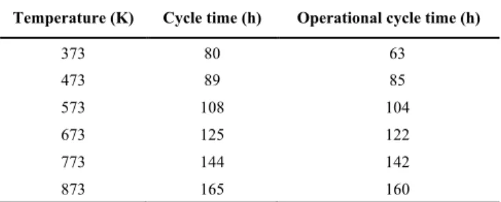
Investigating the effect of temperature on the cycle time and the operational cycle time is important in designing the carbonation operation. The observed cycle times and the operational cycle times for each simulated temperature are shown in Table 4.

Table 4. The effect of temperature on the cycle time and the operational cycle time

Temperature (K) Cycle time (h) Operational cycle time (h)

373 80 63

473 89 85

573 108 104

673 125 122

Table 4 shows that as the temperature increases both the cycle time and the operational cycle time increase. Moreover, the difference between the cycle time and the operational cycle time is more pronounced at 373 K with a value of 17 h. For simulated temperatures above 373 K, the difference is around 2-5 h. In order to investigate this phenomenon, the influence of the operating temperature on the evolution of the rate of reaction is investigated. As the temperature increases, the maximum rate of reaction (after initial conditions) reached in each finite volume decreases. This trend explains the increased cycle time with increasing temperature. Although the rate constant increases significantly by the increased temperature (two orders of magnitude increase in rate constant when the temperature is increased by 500 K), the rate of reaction is also influenced by the conversion and the thermodynamic driving force.

To better incorporate the effect of the thermodynamic driving force on the reaction rate, an improvement method is proposed to be added to the simulation. The hypothesis is that the difference between the partial pressure of CO2 in the finite volume i and the equilibrium partial pressure of CO2 will create a driving force on the finite volume i+1 due to the defined flow direction. As a result, the thermodynamic driving force will increase significantly at higher temperatures compared to previous simulations. The reason is that when the reaction is occurring in finite volume i+1, all of the CaO will already be consumed in finite volume i, resulting in a mole fraction of CO2 of 0.15. The outlet gas stream with an increased CO2 concentration of finite volume i will be the input of finite volume i+1, thus it will accelerate the reaction rate in finite volume i+1. The simulation results show that when the thermodynamic driving force for finite volume i+1 is defined through finite volume i, the rate of reaction modeled as zeroth order reaches its maximum value everywhere in the reactor instantaneously. From 0.05 1/s, it demonstrates an exponential decay due to conversion. As a result of this fast reaction, the cycle time is reduced to 120 s. To further improve this method, the initial amount of sorbent in the reactor can be defined in the simulation.

2) Non-isothermal and Isobaric Operation

The simulation is improved by adding the energy balance to construct the temperature profile and to incorporate its influence. During the non-isothermal simulation, the rate constants, the gas phase concentration, and the equilibrium partial pressure of CO2 are defined as functions of temperature. The temperature of the feed gas is chosen as 443 K, which is the typical flue gas temperature of coal-fired power plants. The temperature of the surroundings is chosen as 873 K, as recommended in the literature.

The feed gas is fed at 443 K and it heats up to 873 K due to the heat transfer from surroundings in the first finite volume. Moreover, as the exothermic carbonation reaction proceeds, the temperature is further increased reaching 916 K at 34 h. At 34 h, CaO is fully consumed in the first finite volume and the corresponding reaction rate is 0 1/s. Due to the termination of the reaction, the first finite volume cools down to the temperature of the surroundings. Consecutively, the identical behavior is repeated in all of the finite volumes. Since the thickness and the internal diameter of the tubes are chosen such that the heat transfer to surroundings by convection is of the same order of magnitude with the heat released during the

(12)

trends are almost identical with the isothermal and isobaric operation at 873 K and ambient pressure.

B. Results for Experimental Investigation

The experiments show that the undoped sorbent loses its capacity significantly in the first four cycles from 75% to below 10%. Mg and Ce doped sorbents also lose their activity throughout 10 cycles, however with a lesser difference of 35% and 20%, respectively. On the other hand, the Al-doped sorbent maintains its activity throughout 10 cycles at 50%. Although the initial theoretical capacity utilized is less than the undoped sorbent, doping with Al is beneficial in preserving the activity.

V. CONCLUSION AND FUTURE WORK

In this study, the mass and energy balances for the fixed bed reactor design are solved by discretizing them spatially with the finite volume method. The resulting system of ordinary differential equations is solved using the ode15s solver in MATLAB. The kinetic models for the carbonation of CaO and the calcination of CaCO3 are incorporated in the simulations. The rate of the carbonation reaction depends on the thermodynamic driving force, CaO conversion, and temperature through reaction kinetics. For the isothermal and isobaric operation at 873 K and ambient pressure, the carbonation reaction occurs consecutively in each finite volume. On the other hand, for the isothermal and isobaric operation at 373 K and ambient pressure, the carbonation reaction happens in more than one finite volume at a time. This phenomenon is explained by comparing the residence and the reaction times. Moreover, it is observed that as the temperature increases, the cycle time and the operational cycle time also increase. In order to investigate this phenomenon, the influence of the operating temperature on the evolution of the rate of reaction is examined. The results show that at as the temperature increases, the rate of reaction decreases as a combined effect of the three constituents of the rate equation. To better incorporate the effect of the thermodynamic driving force, the force exerted from the previous finite volume is applied to the actual finite volume as an improvement proposal. The results demonstrate an increased rate of reaction due to the increased thermodynamic driving force at 873 K compared to previous simulations. Furthermore, the non-isothermal and isobaric operation behaves similarly to the isothermal and isobaric operation due to the thickness and the internal diameter of the tubes, which enable the heat transfer to surroundings by convection to be at the same order of magnitude with the heat released during the exothermic carbonation reaction. The experimental investigation reveals that doping with supports, especially with Al, is beneficial in preserving the activity of the CaO sorbent.

The biggest bottleneck encountered during this study was defining the relationship between the kinetic models and the mass balances. As the future work, the initial amount of CaO in the reactor can be defined in the simulation which could increase the accuracy of determining the cycle time and the operational cycle time. The momentum balance can be added to the simulations to construct the pressure profile and to incorporate its effects on variables such as the thermodynamic driving force and the total gas concentration. The change in the

integration possibilities between the exothermic carbonation and the endothermic calcination reactions can be investigated.

ACKNOWLEDGMENTS

This work is funded by the Master Mind Scholarship from the Government of Flanders.

REFERENCES

[1] Metz, B., Davidson, O., De Coninck, H., Loos, M., & Meyer, L. (2005). IPCC special report on carbon dioxide capture and storage. Intergovernmental Panel on Climate Change, Geneva (Switzerland). Working Group III.

[2] International Energy Agency, United Nations Industrial Development Organization. (2011). Technology Roadmap Carbon Capture and Storage in Industrial Applications.

[3] Blamey, J., Anthony, E. J., Wang, J., & Fennell, P. S. (2010). The calcium looping cycle for large-scale CO2 capture. Progress in Energy and Combustion Science, 36(2), 260-279.

[4] Goto, K., Yogo, K., & Higashii, T. (2013). A review of efficiency penalty in a coal-fired power plant with post-combustion CO2 capture. Applied Energy, 111, 710-720.

[5] Romano, M. C. (2012). Modeling the carbonator of a Ca-looping process for CO2 capture from power plant flue gas. Chemical Engineering Science, 69(1), 257-269.

[6] Markewitz, P., Kuckshinrichs, W., Leitner, W., Linssen, J., Zapp, P., Bongartz, R., ... & Müller, T. E. (2012). Worldwide innovations in the development of carbon capture technologies and the utilization of CO 2. Energy & environmental science, 5(6), 7281-7305.

[7] MacDowell, N., Florin, N., Buchard, A., Hallett, J., Galindo, A., Jackson, G., ... & Fennell, P. (2010). An overview of CO 2 capture technologies. Energy & Environmental Science, 3(11), 1645-1669. [8] Wenzel, M., Rihko-Struckmann, L., & Sundmacher, K. (2018).

Continuous production of CO from CO2 by RWGS chemical looping in fixed and fluidized bed reactors. Chemical Engineering Journal, 336, 278-296.

[9] Spallina, V., Marinello, B., Gallucci, F., Romano, M. C., & Annaland, M. V. S. (2017). Chemical looping reforming in packed-bed reactors: modelling, experimental validation and large-scale reactor design. Fuel Processing Technology, 156, 156-170.

[10] Fedunik-Hofman, L., Bayon, A., & Donne, S. W. (2019). Kinetics of Solid-Gas Reactions and Their Application to Carbonate Looping Systems. Energies, 12(15), 2981.

[11] Emad, S., Hegazi, A. A., El-Emam, S. H., & Okasha, F. M. (2017). Dynamic model of calcium looping carbonator using alternating bubbling beds with gas switching. Fuel, 208, 522-534.

[12] Sun, P., Grace, J. R., Lim, C. J., & Anthony, E. J. (2008). Determination of intrinsic rate constants of the CaO–CO2 reaction. Chemical Engineering Science, 63(1), 47-56.

[13] Martínez, I., Grasa, G., Murillo, R., Arias, B., & Abanades, J. C. (2012). Kinetics of calcination of partially carbonated particles in a Ca-looping system for CO2 capture. Energy & Fuels, 26(2), 1432-1440.

[14] Ergun, S. (1952). Fluid flow through packed columns. Chem. Eng. Prog., 48, 89-94.

[15] Mears, D. E. (1971). The role of axial dispersion in trickle-flow laboratory reactors. Chemical Engineering Science, 26(9), 1361-1366. [16] Gierman, H. (1988). Design of laboratory hydrotreating reactors: scaling

down of trickle-flow reactors. Applied Catalysis, 43(2), 277-286. [17] Froment, G. F., Bischoff, K. B., & De Wilde, J. (1990). Chemical

reactor analysis and design (Vol. 2). New York: Wiley.

[18] Szekely, J., Evans, J. W., & Sohn, H. Y. (1976). Gas-solid reactions Academic Press. New York.

(13)

2.2 CALCIUM LOOPING ... 21 2.2.1 Process Description ... 21 2.2.2 Thermal Integration ... 23 2.2.3 Reactor Technology ... 24 2.2.4 Sorbent Properties ... 27 2.2.5 Pilot Plants ... 29 3 METHODOLOGY ... 31 3.1 MASS BALANCES ... 32 3.2 ENERGY BALANCES ... 33 3.3 KINETIC MODELS ... 34 3.3.1 Carbonation ... 34 3.3.2 Calcination ... 37 4 EXPERIMENTAL INVESTIGATION ... 38

(14)

4.1 DETERMINATION OF THE REACTION ORDER ... 39

4.2 DETERMINATION OF THE KINETIC PARAMETERS ... 40

4.3 SORBENT ENHANCEMENT ... 40

5 RESULTS AND DISCUSSION ... 42

5.1 SIMULATION RESULTS FOR THE CARBONATOR REACTOR DESIGN ... 42

5.1.1 Isothermal and Isobaric Operation ... 43

5.1.2 Non-isothermal and Isobaric Operation ... 55

5.2 RESULTS FOR THE EXPERIMENTAL INVESTIGATION ... 57

5.2.1 Sorbent Enhancement ... 57

6 CONCLUSION AND FUTURE WORK ... 59

7 REFERENCES ... 61

ANNEX A. MASS BALANCES ... 70

A.1.GAS PHASE MASS BALANCE ... 70

ANNEX B. HEAT BALANCE ... 72

(15)

LIST OF FIGURES

Figure 1. Global energy demand by sector (ExxonMobil, 2019) ... 1

Figure 2. Trajectory of the energy sources (ExxonMobil, 2019) ... 2

Figure 3. CO2 concentration in the atmosphere (U.S. Department of Commerce National Oceanic and Atmospheric Administration Earth System Research Laboratory Global Monitoring Division, 2019) ... 3

Figure 4. Global annual temperature anomaly (National Aeronautics and Space Administration [NASA], 2019) ... 3

Figure 5. Global fossil fuel and industry emissions in 2014 (Davis et al., 2018) ... 4

Figure 6. Industrial CO2 emission projections in the ETP Baseline Scenario (International Energy Agency, United Nations Industrial Development Organization, 2011) ... 5

Figure 7. Energy related CO2 emissions (IEA,2019) ... 6

Figure 8. Post-conversion capture (Cuéllar-Franca & Azapagic, 2015) ... 9

Figure 9. Pre-conversion capture (Cuéllar-Franca & Azapagic, 2015) ... 10

Figure 10. Oxy-fuel combustion capture (Cuéllar-Franca & Azapagic, 2015) ... 11

Figure 11. Absorption process diagram (Kenarsari et al., 2013) ... 13

Figure 12. Pressure swing adsorption (Aaron & Tsouris, 2005) ... 15

Figure 13. Membrane separation process (Wang, Zhao, Otto, Robinius & Stolten, 2017) ... 16

Figure 14. Hydrate-based separation process (Wang et al., 2013) ... 17

Figure 15. Cryogenic distillation process (Aaron & Tsouris, 2005) ... 18

Figure 16. Potential combustion process using calcium looping (Blamey et al., 2010) ... 19

Figure 17. Calcium looping process flow diagram (Romano et al, 2012)] ... 22

Figure 18. Equilibrium vapour pressure of CO2 over CaO as a function of temperature (Silcox et al., 1989) ... 23

Figure 19. Moving bed reactor (Moran & Henkel, 2000) ... 25

Figure 20. Rotary kiln (Moran & Henkel, 2000) ... 25

Figure 21. Fluidized bed reactor (Moran & Henkel, 2000) ... 26

Figure 22. Multitubular fixed bed reactor (Moran & Henkel, 2000) ... 26

Figure 23. The simulation algorithm ... 32

Figure 24. Schematic representation of CaO undergoing carbonation and calcination reactions [Fedunik-Hofman et al., 2019] ... 35

Figure 25. Schematic representation of the grain model ... 35

(16)

Figure 27. Simulation scheme for the carbonator reactor ... 42 Figure 28. Simulation results for isothermal and isobaric operation at 873 K and ambient pressure. a) Temperature (K) with respect to time (h) b) Rate of reaction (1/s) with respect to time (h) c) Thermodynamic driving force (Pa) with respect to time (h) d) Mole fraction of CO2

(-) with respect to time (h) e) Mole fraction of CaO (-) with respect to time (h) f) Mole fraction of CaCO3 (-) with respect to time (h) ... 44

Figure 29. Mole fraction of CO2 (-) throughout the reactor length (m) for isothermal and isobaric operation at 873 K and ambient pressure ... 46 Figure 30. Simulation results for isothermal and isobaric operation at 373 K and ambient pressure. a) Temperature (K) with respect to time (h) b) Rate of reaction (1/s) with respect to time (h) c) Thermodynamic driving force (Pa) with respect to time (h) d) Mole fraction of CO2

Figure 31. Mole fraction of CO2 (-) throughout the reactor length (m) for isothermal and isobaric operation at 373 K and ambient pressure ... 50 Figure 32. The evolution of rate of reaction (1/s) with respect to time (h) at different temperatures (K). a) T=373 K, b) T=473 K, c) T=573 K, d) T=673 K, e) T=773 K ... 52 Figure 33. The simulation results of the improvement proposal for isothermal and isobaric operation at 873 K and ambient pressure a) Temperature (K) with respect to time (s) b) Rate of reaction (1/s) with respect to time (s) c) Thermodynamic driving force (Pa) with respect to time (s) d) Mole fraction of CO2 (-) with respect to time (s) e) Mole fraction of CaO (-) with respect

to time (s) f) Mole fraction of CaCO3 (-) with respect to time (s) ... 54

Figure 34. The simulation results for non-isothermal and isobaric operation at ambient pressure a) Temperature (K) with respect to time (h) b) Rate of reaction (1/s) with respect to time (h) c) Thermodynamic driving force (Pa) with respect to time (h) d) Mole fraction of CO2 (-) with

respect to time (h) e) Mole fraction of CaO (-) with respect to time (h) f) Mole fraction of CaCO3 (-) with respect to time (h) ... 56

Figure 35. Durability and capacity of doped and undoped CaO ... 57 Figure 36. Simulation results for isothermal and isobaric operation at 473 K and ambient pressure. a) Temperature (K) with respect to time (h) b) Rate of reaction (1/s) with respect to time (h) c) Thermodynamic driving force (Pa) with respect to time (h) d) Mole fraction of CO2

(17)

Figure 37. Simulation results for isothermal and isobaric operation at 573 K and ambient pressure. a) Temperature (K) with respect to time (h) b) Rate of reaction (1/s) with respect to time (h) c) Thermodynamic driving force (Pa) with respect to time (h) d) Mole fraction of CO2

(18)

LIST OF TABLES

Table 1. CO2 concentration of the flue gases (Davidson & Thambimuthu, 2005) ... 5

Table 2. Carbon capture strategies (Markewitz et al., 2012; Leung, 2014) ... 11

Table 3. CO2 separation technologies ... 12

Table 4. Performance parameters of different CO2 separation technologies ... 20

Table 5. Comparison of potential sorbent materials (Salaudeen et al., 2018) ... 28

Table 6. Comparison of calcium looping pilot plants ... 30

Table 7. Kinetic parameters by Sun et al. (2008) ... 36

Table 8. Experiments for the determination of reaction order ... 40

Table 9. Experiments for the determination of kinetic parameters ... 40

Table 10. The effect of temperature on the cycle time and the operational cycle time ... 51

Table 11. Physical and thermodynamic properties and design specifications used in mass balances ... 71

Table 12. Physical and thermodynamic properties and design specifications used in heat balance ... 74

(19)

LIST OF ABBREVIATIONS

Al Aluminum

BFB Bubbling fluidized bed

BTU British thermal unit

Ca Calcium

CaCO3 Calcium carbonate

CaO Calcium oxide

Ce Cerium

CFB Circulating fluidized bed

CO Carbon monoxide

CO2 Carbon dioxide

DEA Diethanolamine

ETP Energy Technology Perspective

H2 Hydrogen H2O Water H2S Hydrogen sulfide He Helium MEA Monoethanolamine MDEA Methyldiethanolamine Mg Magnesium N2 Nitrogen

N/A Not available

NOx Nitrogen oxides

O2 Oxygen

ODE Ordinary differential equation

SiC Silicon carbide

SOx Sulfur oxides

SO2 Sulfur dioxide

STP Standard temperature and pressure

(20)

LIST OF SYMBOLS

Roman Symbols

Symbol Description Units

𝐵𝑖 Biot number -

𝐶_$,&'( specific heat capacity of CaO J/mol/K 𝐶_$,&'&(₎ specific heat capacity of CaCO3 J/mol/K

𝐶_$,&(_* specific heat capacity of CO2 J/mol/K

𝐶_$,+_* specific heat capacity of N2 J/mol/K

𝐶_$,, specific heat capacity of the gas phase J/mol/K

𝐶$,- specific heat capacity of the solid phase J/mol/K

𝑐/,, total gas concentration mol/m3

𝑑 particle diameter m

𝐷₂₃ Knudsen diffusivity of CO2 into CaO m2/s

𝐷₄ effective diffusion coefficient m2_/s

𝑑_45/ external tube diameter m

𝐸 activation energy kJ/mol

ℎ₈ wall heat transfer coefficient W/m2_/K

𝑘_: pre-exponential factor mol/m2_/s/Pan

𝑘:; kinetic constant mol/m2/s

𝑘_<'=< reaction rate constant for calcination m3_/mol/s

𝑘_<'>? reaction rate constant for carbonation mol/m2_/s/Pan

𝑘&'( thermal conductivity of CaO W/m/K

𝑘_&'&(₎ thermal conductivity of CaCO3 W/m/K

𝑘_&(_* thermal conductivity of CO2 W/m/K

𝑘₊_* thermal conductivity of N2 W/m/K

𝑘_, thermal conductivity of the gas phase W/m/K

𝑘_- thermal conductivity of the solid phase W/m/K

𝑀&'( molar weight of CaO kg/mol

𝑀_A molar mass of component 𝛽 kg/mol

(21)

𝑃_&(_* partial pressure of CO2 Pa

𝑃_&(_*_,4G equilibrium partial pressure of CO2 Pa

𝑃𝑒_'5 axial Peclet number -

𝑃𝑟 Prandtl number -

𝑟 constant -

𝑅 specific reaction rate 1/s

𝑅,'- ideal gas constant m3Pa/K/mol

𝑅𝑒 Reynolds number

-𝑆 surface area of the sorbent m2_/kg

𝑡 time s

𝑇 temperature K

𝑇_45/ temperature of the surroundings K

𝑥_&'( molar fraction of CaO -

𝑥&'&() molar fraction of CaCO3 -

𝑋_&'( conversion of CaO -

𝑋_&'&(₎ conversion of CaCO3 -

𝑥_&(_* molar fraction of CO2 -

𝑥₊_* molar fraction of N2 -

𝑥_P(R) mole fraction of the gas component 𝛼 -

𝑋 conversion -

𝑋_A conversion of component 𝛽 -

𝑧 distance m

Greek Symbols

Symbol Description Units

𝛼 component in the gas phase -

𝛽 component in the solid phase -

Δ𝐻_X enthalpy of reaction J/mol

𝜀, fixed bed void fraction -

𝜀_- solid porosity -

𝜂_4[[ effectiveness factor -

(22)

𝜆_'5 axial heat dispersion W/m/K

𝜆_?4^,: heat dispersion of the bed W/m/K

𝜆_, heat dispersion of the gas phase W/m/K

𝜇_, dynamic viscosity of the gas phase N.s/m2

𝜇&(* dynamic viscosity of CO2 N.s/m2

𝜇+* dynamic viscosity of N2 N.s/m2

𝜈_P stoichiometric coefficient of the component 𝛼 -

𝜌_&'( density of CaO kg/m3

𝜌&'&() density of CaCO3 kg/m3

𝜌_&(_* density of CO2 kg/m3

𝜌+* density of N2 kg/m3

𝜌- density of the solid phase kg/m3

𝜌_, density of the gas phase kg/m3

𝜎_< constriction factor -

(23)

1 INTRODUCTION

Global climate change is a concerning threat to life on Earth. The rise in global temperatures, warming of the oceans, shrinking ice sheets, sea-level rise, extreme events such as intense rainfalls, and ocean acidification are primary evidences of global warming. Anthropological sources like burning of fossil fuels for power generation vastly induce global warming by emitting greenhouse gases. Reduction in agricultural yields, limited access to clean water, flooding of residential areas, and extinction of wildlife are a few of the major consequences of climate change that require immediate and effective action.

1.1.1 Global Energy Demand

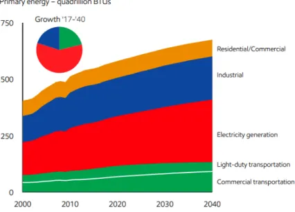
The global energy demand continues to grow with the increase in population, growing prosperity especially due to emerging economies, and higher heating and cooling needs in certain parts of the world. The global consumption of energy increased 2.3% since 2010. Electricity generation is responsible for half of this growth (International Energy Agency [IEA], 2019). Figure 1 demonstrates the projected change in energy demand by sectors over 40 years (ExxonMobil, 2019).

Figure 1. Global energy demand by sector (ExxonMobil, 2019)

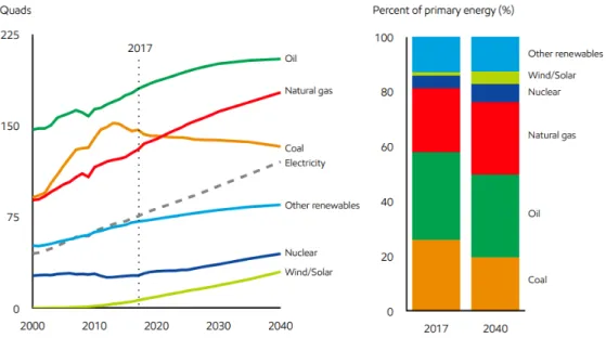
To be able to supply for this demand, the efficient use of primary energy sources is vital. Figure 2 shows the trajectory for 2040 and it indicates that fossil fuels, namely oil, natural gas, and coal will continue their leading role as primary energy sources (ExxonMobil, 2019).

(24)

Figure 2. Trajectory of the energy sources (ExxonMobil, 2019)

1.1.2 Greenhouse Gas Emissions

As mentioned in the previous section, with the increase in the use of fossil fuels as primary energy sources, global warming continues to be a growing and concerning issue. The combustion of fossil fuels emits greenhouse gases which has been proven to be the primary reason for climate change. A greenhouse gas is a gas that absorbs and emits radiation within the thermal infrared spectrum. The primary greenhouse gases in the atmosphere consist of carbon dioxide, methane, nitrous oxide, and fluorinated gases. Since the Industrial Revolution, the concentration of greenhouse gases in the Earth’s atmosphere has been rising steadily and the mean global temperature is also following this trend which is depicted in Figures 3 (U.S. Department of Commerce National Oceanic and Atmospheric Administration Earth System Research Laboratory Global Monitoring Division, 2019) and 4 (National Aeronautics and Space Administration [NASA], 2019) .

(25)

Figure 3. CO2 concentration in the atmosphere (U.S. Department of Commerce National Oceanic and Atmospheric

Administration Earth System Research Laboratory Global Monitoring Division, 2019)

Figure 4. Global annual temperature anomaly (National Aeronautics and Space Administration [NASA], 2019)

The average global temperature is directly linked to the concentration of greenhouse gases in the Earth’s atmosphere and the most abundant one is CO2, accounting for around two-thirds of

the total (United Nations [UN], 2019). Due to the increased energy demand and the growth in consumption of fossil fuels, energy-related CO2 emissions increased by 1.7% reaching the

highest level of all times at 33.1 Gt CO2 in 2018. It is the fastest rate in growth since 2013 and

(26)

for 30% of these emissions, being the largest single emitter (IEA, 2019). The International Energy Agency (2019) found out that coal combustion is accountable for over 0.3°C of the 1°C rise in global average annual surface temperatures above pre-industrial levels. Furthermore, a quarter of the worldwide CO2 emissions are attributed to total industry and fuel transformation.

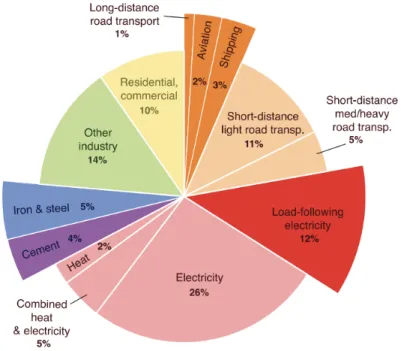
Figure 5 shows the distribution of CO2 emissions among various sectors ranging from

electricity production to transportation. As it can be seen, electricity accounts for 26% of overall CO2 emissions, thus focusing on emission reductions from power plants is significant

(Davis et al., 2018).

Figure 5. Global fossil fuel and industry emissions in 2014 (Davis et al., 2018)

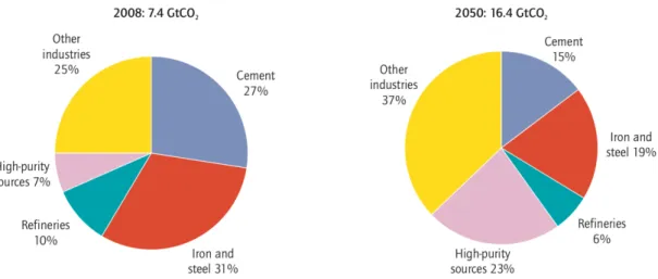
The main industrial sources and fuel transformation processes for CO2 emissions and their

projections in the Energy Technology Perspective (ETP) Baseline Scenario are represented in Figure 6 (International Energy Agency, United Nations Industrial Development Organization, 2011). The ETP Baseline Scenario assumes no additional policies are implemented on the current status regarding emission reductions (UN, 2019). The key finding of the ETP Baseline Scenario is that CO2 emissions increase by 120% from the total industry and fuel transportation

sectors by 2050. It is important to mention that biomass conversion is not included in this analysis (International Energy Agency, United Nations Industrial Development Organization, 2011).

(27)

Figure 6. Industrial CO2 emission projections in the ETP Baseline Scenario (International Energy Agency, United Nations

Industrial Development Organization, 2011)

Flue gases of high-purity sources have CO2 concentrations ranging between 80 vol% to 99

vol% and they are typically available from natural gas processing, hydrogen production from natural gas, coal or biomass, and ethylene oxide and ammonia production. The CO2 level in the

combustion flue gas is typically at 12-14 vol% for coal-fired and 10 vol% for gas-fired power plants (Song et al., 2004). CO2 concentration in flue gas is an important parameter in

determining the separation technology to be used, so it is important to distinguish between compositions of flue gases from different industries. Typical CO2 concentrations of flue gases

from major sources shown on Figure 6 are presented in Table 1 (Davidson & Thambimuthu, 2005). In refineries, there are various CO2 sources with different concentrations.

Table 1. CO2 concentration of the flue gases (Davidson & Thambimuthu, 2005)

Industry CO2 Concentration in Flue Gas (vol%)

Cement 14-33

Iron and steel 20

Refinery 8-20

High-purity sources 80-99

1.1.3 The Role of Carbon Capture

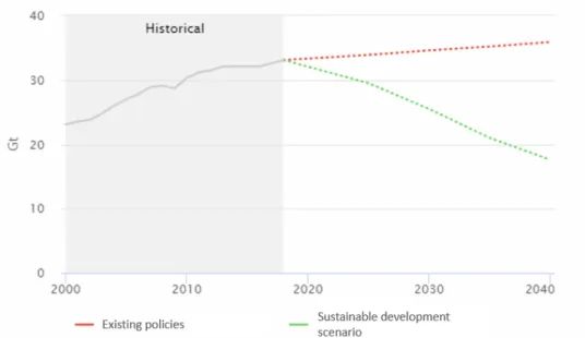
The Paris Agreement aims to limit global warming to 2°C above pre-industrial levels and carbon capture and storage technologies play a vital role in achieving this goal (Nookuea, Tan, Li, Thorin & Yan, 2016). Figure 7 compares the energy-related emissions of existing policies and the sustainable development scenario (IEA,2019).

(28)

Figure 7. Energy related CO2 emissions (IEA,2019)

Carbon capture and storage is a promising technology which aims at minimizing the effects of CO2 emissions. The Intergovernmental Panel on Climate Change states that the cost of limiting

CO2 concentrations to 430-480 ppm in the atmosphere would be 138% higher without the

large-scale deployment of carbon capture and storage systems for the 2°C scenario (Metz, Davidson, De Coninck, Loos & Meyer, 2005). In industrial applications, carbon capture and storage could decrease CO2 emissions by up to 4 gigatonnes per year by 2050, accounting for almost 9% of

the reductions required to halve the energy-related emissions. In order to achieve this, carbon capture and storage processes are needed to be implemented in 20% to 40% of all power plants by 2050 (International Energy Agency, United Nations Industrial Development Organization, 2011). As of 2020, 19 large scale carbon capture and storage facilities are in operation and four more are in construction worldwide. Of these 19 operating facilities, two are in the field of power generation (Global Carbon Capture and Storage Institute, 2019). The relatively high capital and operating costs of carbon capture methods in fossil fuel power plants are causing delays in commercialization. The reasons for the high capital costs are the size of units required to accommodate the flue gas volume and the energy penalty (Hanak, Biliyok, Anthony & Manovic, 2015). The energy penalty is the reduction in the net efficiency of the power plant due to the energy requirements associated with CO2 capture and compression processes (Goto,

Yogo & Higashii, 2013). The capture step is the costliest and most energy-intensive stage of the carbon capture and storage process, therefore the focus is on reducing the costs through different technologies and materials. Chemical and physical absorption, adsorption, cryogenic

(29)

separation, hydrate-based separation, the use of membranes, and calcium looping are the most well-known methods to capture CO2.

1.1.4 Aim of the Project

This project aims to develop a large-scale reactor model for the gas-solid calcium looping process to capture and separate CO2 from an industrial gas stream. The learning objectives

consist of acquiring knowledge about various carbon capture methods, specifically focusing on the calcium looping process, investigating potential reactor types for gas-solid reactions, developing a readable reactor model using MATLAB for the selected reactor type, and optimizing process conditions.

(30)

2 LITERATURE REVIEW

2.1 Carbon Capture, Storage, and Utilization

Carbon capture and storage consists of the separation of CO2 from industrial and energy-related

sources, transportation to a storage site, and long-term isolation from the atmosphere up to thousands of years (Metz et al., 2005). The capture stage removes CO2 from other gases

produced at large industrial processes, such as coal and natural gas-fired power plants, the steel and cement industry, and refineries. After capture, CO2 is further compressed and transported.

Transportation is done via pipelines, trucks, ships, or alternative methods that are applicable to geological storage. Finally, CO2 is injected into deep underground rock formations to be stored

geologically (Global Carbon Capture and Storage Institute, 2019). As an alternative, captured CO2 can also be directly utilized. Carbon capture and utilization offers the opportunity to

economically make use of CO2 emissions by closing the carbon cycle above the ground (Group

of Scientific Advisors, 2018).

2.1.1 Carbon Capture Technologies

Power plants, oil refineries, natural gas processing, ammonia and ethylene oxide production, and cement, iron, and steel industries are the main industrial sources of CO2 emissions, so these

are the most significant areas for potential applications of carbon capture technologies (International Energy Agency, United Nations Industrial Development Organization, 2011). Due to the diversity of application areas, different carbon capture implementation techniques are needed. However, capture systems vary in maturity across industries. As an example, large-scale implementations of carbon capture systems in power plants and oil refineries are beginning to be commercialized. On the other hand, cement, iron, and steel industries are still in the scale-up phase (Cuéllar-Franca & Azapagic, 2015). Carbon capture strategies can be classified into three groups, namely post-conversion, pre-conversion, and oxy-fuel combustion according to wherein they are implemented in the process flow. The concentration of CO2 in

the gas stream, the pressure of the gas stream, and the fuel type are significant parameters in choosing the capture system (Metz et al., 2005).

2.1.1.1 Post-Conversion Capture

Post-conversion capture is the separation of CO2 from the waste gas stream after the conversion

(31)

to achieve the highest CO2 purity among all capture methods which is above 95 mol%. Still,

the large energy penalty is the most important drawback of this method. The efficiency loss of a power plant due to post-combustion capture is typically around 10-12% (Markewitz et al., 2012). In utilizing the absorption by solvents method, the absorber of the post-combustion absorption unit would consume a quarter to one-third of the total steam produced by the plant, consequently decreasing its generating capacity by the same value. Due to this, research estimates that the cost of electricity would increase by 70% with post-combustion capture including the compression stage (Elwell & Grant, 2006). An economic study states that the cost of electricity would rise by 32% and 65% for post-combustion in gas and coal-fired plants, respectively (Kanniche, 2010). Therefore, research is focused on improving post-combustion capture in a cost-effective way (Leung, Caramanna & Maroto-Valer, 2014). The block diagram of post-conversion capture is represented in Figure 8 Cuéllar-Franca & Azapagic, 2015).

Figure 8. Post-conversion capture (Cuéllar-Franca & Azapagic, 2015)

2.1.1.2 Pre-Conversion Capture

Pre-conversion capture consists of reacting a carbonaceous fuel with O2 or steam to produce

mainly syngas or fuel gas composed of CO, H2,and trace amounts of H2O and H2S. When

steam is used, the reaction is called steam reforming (displayed in Equation 1 below) and when O2 is used, it is called partial oxidation (displayed in Equation 2 below) in the case of gaseous

or liquid fuels and gasification in the case of solid fuels. Generally, the carbonaceous fuel is either coal or natural gas. The formed CO is further reacted with steam in a catalytic reactor to produce CO2 and more H2. This reaction is called the water-gas shift reaction (displayed in

Equation 3 below). The concentration of CO2 in this mixture is 15-60 vol% (dry basis) at a total

pressure typically at 2-7 MPa (Jansen, Gazzani, Manzolini, van Dijk & Carbo, 2015). From this mixture, CO2 is separated easily and in a cost-efficient manner due to the lack of N2

(32)

(Kanniche et al., 2010). Usually, CO2 is separated by physical or chemical absorption at around

ambient temperatures, resulting in an H2-rich fuel which can be utilized in many areas such as

boilers, furnaces, gas turbines, engines, and fuel cells (Jansen et al., 2015). The corresponding reaction equations are as follows,

Steam reforming: 𝐶₅𝐻_e + 𝑥𝐻_g𝑂 ↔ 𝑥𝐶𝑂 + k𝑥 +𝑦 2n 𝐻g (1) Partial oxidation: 𝐶₅𝐻_e+5_g𝑂_g ↔ 𝑥𝐶𝑂 +e_g𝐻_g (2) Water-gas shift: 𝐶𝑂 + 𝐻_g𝑂 ↔ 𝐶𝑂_g+ 𝐻_g , ∆𝐻_: = −41 𝑘𝐽𝑚𝑜𝑙_&(xy (3)

This technology applies to integrated gasification combined-cycle power plants using coal as fuel with the capture efficiency of 80% (Markewitz et al., 2012). An efficiency loss of 7-8% will be caused by this implementation (Leung et al., 2014). Pre-conversion capture can also be applied to natural gas power plants. In a process called autothermal methane steam reforming, the oxygen burns a part of the methane to create heat that drives the main endothermic steam methane reforming reaction, forming syngas. Again, with the shift reaction, CO2 is produced

from CO, consequently, a stream that mostly consists of H2 and CO2 is formed (Kenarsari et

al, 2013). The block diagram of the pre-conversion capture is shown in Figure 9.

Figure 9. Pre-conversion capture (Cuéllar-Franca & Azapagic, 2015)

2.1.1.3 Oxy-Fuel Combustion Capture

O2, instead of air, is used in oxy-fuel combustion. Due to the elimination of N2 resulting in a

smaller volume of gases, the combustors are smaller but more complex compared to combustion with air. When fuel is burned with pure O , the combustion temperature is higher,