Netherlands Environmental Assessment Agency, P.O. Box 303, NL-3720 AH BILTHOVEN The Netherlands, ph +31 30 274 4529
Report 773001033/2006
The PIE information system
Platform on Integral Energy and emission Projections
- Technical description -
A Gijsen*, R A van den Wijngaart*, B W Daniels**
* Netherlands Environmental Assessment Agency (MNP)
The Netherlands Environmental Assessment Agency (MNP) is one the four independent assessment agencies in the Netherlands. These agencies all have a role to play in giving substance to the World Bank’s People-Planet-Profit concept, with the Social and Cultural Planning Office of the Netherlands (SCP) dealing with ‘People’, the Netherlands Bureau for Economic Policy Analysis (CPB), with ‘ Profit’ and the Netherlands Environmental Assessment Agency (MNP), along with the Netherlands Institute for Spatial Research (RPB), with the ‘Planet’.
** ECN Policy Studies
The Energy Research Centre of the Netherlands (ECN) Policy Studies provides independent advice to the public and private sectors with respect to energy and environmental issues. Innovation in the area of policy studies is primarily aimed at strengthening the synergy between market forces and sustainability. The multidisciplinary project teams provide advice at a local, national and international level, and make use of a wide range of up-to-date models and data to support the recommendations.
This research has been carried out in the framework of the project ‘Models and Policy Recommendations’, number 773001.
Abstract
The PIE information system
The information system, Platform on Integral Energy and emission projections (PIE) described here, has been developed by the Netherlands Environmental Assessment Agency (MNP) and the Netherlands Energy Research Centre (ECN), two Dutch research centres with overlapping interests in the area of energy and emission projections. PIE has been set up to share data common to both centres and as a means of responding to policy questions with greater speed, flexibility and insight. This report first of all describes the history and purpose of PIE before providing an explanation of the conceptual model. This is followed by a discussion of the conceptual model’s implementation in Excel and the mathematical rules connected with its use. The final chapter discusses plans for PIE application in the near future.
Key words: energy, emissions, platform, scenario
Rapport in het kort
Platform Integrale Energie- en Emissieverkenningen
Dit rapport beschrijft het informatiesysteem genaamd Platform voor Integrale Energie- en emissieverkenningen (PIE). Omdat het MNP en ECN een cruciaal raakvlak hebben op het terrein van energie en emissies werken zij gezamenlijk aan de ontwikkeling en het gebruik van het Platform voor Integrale Energie- en Emissieverkenningen. PIE dient bij te dragen aan enerzijds het vastleggen van gezamenlijke informatie en anderzijds aan flexibeler, sneller en inzichtelijker beantwoorden van beleidsvragen. Dit rapport geeft allereerst een beschrijving van de historie en het doel van PIE. Vervolgens wordt het conceptuele model uitgelegd. De toepassing van het conceptuele model in Excel en de daarmee samenhangende rekenregels worden toegelicht en er wordt afgesloten met een beschrijving van de te nemen vervolgstappen.
Contents
1 Introduction 7
2 Description of the model 13 3 PIE-Excel 19
3.1 Introduction 19
3.2 Energy demand from end-use sectors 20 3.3 Energy supply Conversion sector 26
3.4 Linking supply to demand: ‘Useful to Final’ sheet 30 3.5 Emissions from the Conversion sector 34
3.6 Emissions from the end-use sectors 35
4 Conclusions and follow-up 37 List of tables and figures 39
Reference 41 Appendix A 43
1
Introduction
This report describes the information system ‘Platform on Integral Energy and emission projections’ (PIE) that focuses on energy supply and demand, as well as the emissions related to these at a national level. This introduction details the background to and purpose of PIE. Chapter 2 provides a general description of PIE. Chapter 3 provides a description of the PIE model as implemented in Excel. The structure of the model is detailed and several formulae are also presented.
Background to the cooperation between MNP and ECN
Several years ago MNP acquired the ‘Reken en Informatie Model’ (RIM+) (Calculation and Information Model) as a tool for emission prognoses. However, this model was found to have shortcomings with respect to answering various questions concerning energy use and emissions. Accordingly MNP is looking to build a new model for energy provision. At the same time ECN wants to make its models more efficient and accessible so as to improve the flexibility and speed with which global results can be obtained. This will also mean that staff other than modelling experts will be able to run the models and make more general analyses. As there is a considerable overlap between MNP’s and ECN’s research interests in the area of energy and emissions, they are working together on the development and use of the Platform on Integral Energy and emission projections (PIE). On the one hand, PIE should contribute to establishing a joint pool of data and, on the other hand, to providing greater flexibility, speed and insight in answering policy questions.
Objective of the PIE platform
PIE has a strong integral function across the chain from economics via energy supply and demand to the associated emissions. In the first place, PIE can be used to calculate the consequences of changes in the energy demand (services) on emissions further up the chain. An example of this is the change in mobility and vehicle technology; a shift from combustion engines to electric motors (batteries and fuel cells) can be expressed in terms of emissions within the traffic sector as well as in the production sectors of electricity, biofuels and hydrogen. A second integral aspect is the simultaneous inclusion of all relevant energy emissions for climate (CO2) and large-scale air pollution (NOx, SO2,
VOCs and fine particles).
PIE is best classified as a platform as opposed to an endogenous model. Important functions are the accessing of information from existing models and the management of information (more flexible, faster and less ‘black box’ than the present situation). For example, at present, the information from the long-term projections (LT’97, NEV and MV4/5) is distributed over three different institutes (CPB (Netherlands Bureau for Economic Policy Analysis), ECN and MNP) each with its own information systems, submodels, etcetera, the results of which are reported in different documents. New insights, updating of the policy and potential studies such as the new Option document (Sectoral CO2 emissions to 2010 from December 2003 compared to the Reference framework from
January 2002) can be unequivocally included in PIE. Initially the objective was to link submodels (i.e. models on sub-areas) to PIE as well, feeding the outcomes of these to a usually higher aggregated level in PIE. However, due to the frequently complex nature of the submodels and differences in definitions, for example, in the protocol for energy saving, most of the submodels were not linked to PIE. And where submodels are linked, these and not PIE, should be used to obtain more detailed answers.
PIE can be used, for example, to analyse trends in indicators of energy use and emissions, to draw up new scenarios, to describe sensitivities and uncertainties in existing prognoses and to compare the
outcomes from different submodels. In addition to this the model can be unequivocally updated with new insights concerning the economy, energy supply and emissions. Some applications and specifications are:
• calculating the effects of changes in a subarea on the entire energy supply; • calculating the effects of cross-sectoral policy instruments;
• establishing scenarios and constructing variants of these. Attributes of the model
The purpose of the project is to construct a knowledge model with which the entire Dutch energy supply chain can be expressed in terms of energy use, CO2 emission and other emissions (NOx, SO2,
VOCs and fine particles). With this instrument, it should be possible to broadly calculate prognoses and different potential solutions for energy-related emissions. Important aspects include potential, costs and implementation options for different potential solutions and the effectiveness of policy instruments.
Policy-relevant questions
Ultimately the platform should be able to provide answers to a wide range of questions, such as: • What is the final energy demand, and/or energy requirement (distributed over the energy
carriers) for the different target groups?
• What is the overall pattern in the energy supply distribution (electricity and other energy carriers) and what are the resulting emissions?
• What are the patterns for CO2 emissions and the emissions of NOx, SO2, fine particles and VOCs
for the different target groups?
• What different potential solutions can be used to reduce the emissions? What are the reduction potentials and costs (including investment costs, annual costs, cost-effectiveness) of these? What are the associated limiting conditions?
• What are the possible options for government policy? This concerns, for example, the effectiveness of the following four types of policy instruments:
- levies and other fiscal measures; - subsidies;
- marketability;
- non-financial measures (emission standards, legislation, agreements and so forth). The last two aspects have not been included in PIE-Excel version 1.0.
Compounds
The platform considers emissions of CO2, NOx, SO2, VOCs and fine particles associated with energy
used in the Netherlands (energy sector and end-use sectors such as industry, traffic, etcetera)1. Sectors
The end use of energy is distinguished in five sectors with a total of 15 to 20 subsectors. In many cases several indicators are used for the development of the energy demand. The end use is provided for by energy from the energy supply sector, where the subsectors are energy transport/distribution and energy conversion. End use and energy supply together determine the total national use2.
Energy carriers
1 In order to present the total emission, the emissions of CO
2, NOx, SO2, VOCs and fine particles from other sources are included in
the reference scenario. Greenhouse gases other than CO2 are also included for the reference scenario.
2
The energy carriers distinguished are coal, oil, natural gas, electricity, renewable energy (such as wind energy, solar energy and biomass), heat and other sources. For this it should be noted that several energy carriers such as electricity and heat supply are either produced in the Netherlands from other energy sources such as (in part imported) natural gas and biomass, or are directly imported.
Method / structure
The platform, PIE, contains information about reference scenarios within which alternative developments can be worked out in broad terms. The most important steps:
1) PIE contains information about the reference scenario (indicators for energy development); 2) PIE links alternative data (policy, societal and scientific developments);
3) PIE calculates the effects of the alternative data. 1. PIE contains information about the reference scenario
The most important developments for energy and emissions in a reference scenario are stored in PIE. The indicators included are:
• The development of the energy demand by end users. Three developments are distinguished here:
- volume (for example, the growth of goods transport in tonne km);
- dematerialisation (for example, the development in the size of goods compared to their weight);
- energy savings (for example, the development of the capacity utilised). • The energy supply in the projected year is differentiated into:
- the distribution over energy carriers at end use (in the case of traffic for example oil (= petrol/diesel), gas (= LPG), electric transport, ethanol/methanol, hydrogen; the modal split is apparent in this case);
- the efficiency with which the energy source is converted into the previously stated energy demand (for example, the efficiency of the mode of transport such as more energy-efficient combustion engines, electric vehicles and fuel cells);
- the production of energy carriers in the energy supply sector. In a number of cases the energy source is directly imported or obtained; in other cases the energy source is produced from other energy carriers. Characteristics of this energy production have been included for the latter case. This mainly concerns electricity, heat and hydrogen.
• The emission factors of the energy carriers in the projected year which are converted in the sectors.
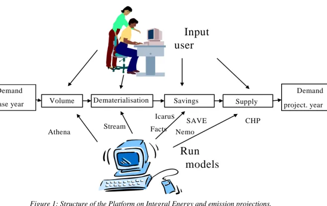
With the help of these characteristics and simple formulae (linear, like addition/subtraction and multiplication/division), PIE can calculate the energy use and emissions in a future year within a reference scenario. First of all, the energy demand in a baseline year is scaled up to the projected year. The total energy use is then determined with the help of the energy supply. Finally the emissions are calculated using the emission factors. The structure of PIE is summarised in Figure 1.
Figure 1: Structure of the Platform on Integral Energy and emission projections. .
2. PIE links alternative data
New insights, variants, potential studies and sensitivity analysis can be included in PIE. Examples are:
a. changes in economic developments such as GNP, physical production, economic structure and energy prices;
b. technical options for energy savings and emission reduction; c. policy instruments.
The alternative data are entered by changing the characteristics of the reference scenario (see 1). The alternative data can be entered manually. These data represent, for example, the results of a submodel (model in a separate sub-area). Originally it was the intention to directly link a number of submodels. With this, detailed results from submodels could be entered into PIE at a higher aggregate level. An example of this is the number of subsectors in ‘SAVE-industrie’ from ECN, which is much larger than in PIE. Due to the complexity of the submodels and the difficulties in overcoming differences in definitions between the submodels and PIE, the decision to link these submodels was suspended. (A third possibility would have been to include a global relation which describes the results of a submodel at a higher aggregate level).
PIE Structure
Demand
base year Volume Dematerialisation Savings Supply
Demand project. year
Input
user
Run
models
Athena SAVE Facts Nemo CHP Icarus
Stream3. PIE calculates the effects of the alternative data
Energy savings, emission reductions and costs over the entire chain can be determined by comparing the alternative (step 2) with the reference scenario (step 1). Two aspects need to be borne in mind in this respect:
a. PIE makes certain assumptions during the integral calculation of the alternative. Example: if the electricity demand is smaller in the alternative (for example, due to less growth in the ICT sector, increase in the Regulating Energy Tax, less transport per rail) then PIE changes the electricity production from power stations using natural gas (in other words, wind, coal-fired power stations, import, etcetera remain the same as in the reference scenario).
Such assumptions must be explicitly stated during the description of the alternative. b. Indicators may only be changed within certain boundaries. Example:
if an increase of the petrol price leads to a reduction in the number of traffic kilometres, this does not automatically result in a change in other macroeconomic effects (for example, decrease in industrial production). Boundaries to permitted changes of characteristics must be stated as much as possible.
2
Description of the model
This chapter provides an overview of the results of the development of PIE (Platform on Integral Energy and emission projections) and contains a general description of PIE (the conceptual model). A description of the software is given in Chapter 3.
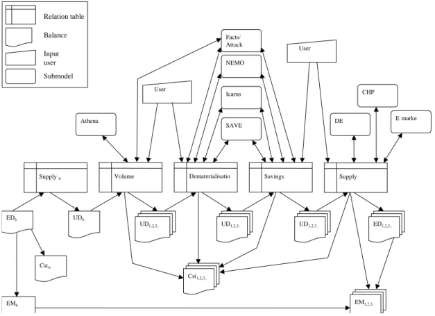
Figure 2: Structure of the energy demand side of PIE.
The primary process of the energy model is formed by linking tables containing energy balances, as shown in Figure 2. The relationships between two consecutive balances are recorded in a so-called relation table. The idea behind the structure of the primary process is that the user’s input, results from submodels, etcetera, are included in the relation tables; the numbers in the balances are derived from the previous balance and the relation table with the help of formulas. Moreover, a choice for this structure does not necessarily mean that the user also sees this structure.
The user will sometimes be interested in the numbers in the balances, yet it is just as likely that other information is being sought. For example, the user is not interested in the contribution of heat energy in the electricity demand but in the capacity and nature of the plants. Such information is made available separately (and is also linked to other parameters via the relation tables) but does not play a role in the rest of the primary process. It can therefore best be described as a sideline with a terminus and not as an intermediate result (transfer point). The same applies to the emissions.
SAVE UD1,2,3.. ED1,2,3.. EDb Supply Savings Dematerialisatio Volume Supplyb EMb Cst1,2,3.. EM1,2,3.. E marke CHP DE Icarus NEMO Athena User Facts/ Attack User UD1,2,3.. UD1,2,3.. UDb Cstb Balance Relation table Input
user Submodel
Energy balances
The following balances are distinguished: • Energy demand baseline year EDb
This is the demand from end users such as households and industry for energy carriers such as natural gas, oil and electricity in the baseline year.
• Useful demand baseline year UDb
This is the energy demand for natural gas, oil, electricity, etcetera, converted into the demand for heat, electricity and raw materials. For example, there is a demand for heat from households, and this can be met by various energy carriers such as natural gas and oil.
• Useful demand projected years after processing volume effects per sector (UD1,2,3,..)
The demand for energy also increases as a result of the growth of the sector. In the households sector, the number of households is increasing and, accordingly, so is the energy demand for the total sector.
• Useful demand projected years after processing dematerialisation (intrasectoral structural effects) per sector (UD1,2,3,..)
A sector can also undergo changes. For example, in the household sector people are making more use of televisions and computers in the evening and books are read less often. This shift has led to a greater demand for energy.
• Useful demand projected years after savings measures (UD1,2,3,..)
Due to a range of measures the demand for energy has decreased. Examples in the household sector are the insulation of homes or more energy-efficient refrigerators.
• Energy demand projected years (ED1,2,3,..)
The useful demand for heat, electricity and raw materials determines which energy source is used to generate the useful demand. In the case of households, the demand for heat can be satisfied with a gas boiler, but also with a wood stove.
The data per sector are presented in each balance. Table 1 shows the sector classification chosen.
Table 1: End-use sectors of PIE
Sector Subsector
Industry Food
Chemical
Primary metals industry Other metal industries Construction materials Printing and paper Refineries Other industry Agriculture Horticulture Other agriculture Transport People Goods
Services Trade and catering
Business services Non-profit sector
Households New buildings
Existing buildings Appliances
The following energy carriers are distinguished in the balances:
Energy demand: coal, oil, natural gas, electricity, renewable, heat and other Useful demand: heat, electricity and raw material
Relation tables
The relation tables contain the data needed to calculate the figures for one balance using the previous balance. These are relative figures such as components in the demand or growth percentages per year. Examples are the economic growth of the baseline industry, the conversion efficiency with which the energy demand from the baseline year is converted into useful demand, the efficiency improvement in a sector, etcetera. However, there is also the case of user (or certain submodel) results which do not directly agree with the parameters stated, and which need to be generated via an extra processing step. If the user wishes to clearly input the quantity of floor surface in hospitals, this will need to be converted by the model into a relationship between economic growth and physical growth, the process which results in (de)materialisation. This will have to take place in an interface between the user or submodel and the relation table.
External input
An existing scenario always forms the starting point for the integral energy model. This means that all of the balances and tables are filled with the applicable value from that scenario. As soon as the user enters new input in the model and/or submodels run with altered input, the figures in the relation tables will change. In principle the user can then see a new outcome immediately (the relation between balances and relation tables is unequivocal). However, it is also the case that the relationships derived using other submodels may no longer apply; for example, the relation tables contain a certain package of fuels for the electricity supply (distribution of coal, oil, gas, renewable and other). This is consequential to existing and new capacity and new buildings. If, as a result of changes elsewhere in the model, the electricity demand suddenly halves, the electricity production using natural gas will be lowered in PIEn. This is because natural gas is assumed to be the balancing item for electricity production. However, a different result can be obtained if the user modifies the characteristics of the electricity supply module.
Supply
After the Useful demand following energy savings measures has been calculated, this useful demand must once again be converted into the demand for the specific energy sources. This is described in the supply section. The useful demand from the end users is the main focus of the supply section. Part of the demand is not realised at the end users but at the central energy supply. This concerns the production of electricity and heat. These energy sources are transported to the end users after their production.
The losses associated with the transport of an energy source to the end users from the moment it is extracted, imported and converted are stated for transport. The losses are expressed as efficiency, which represents the relationship between the unit output by the transport sector (to end users) and the unit input (from extraction, production and import).
The central energy provision concerns the conversion of primary energy carriers into secondary energy carriers. The production of electricity, heat, hydrogen, etcetera takes place within this sector. During the modelling a clear distinction is drawn between the conversion of electricity and the conversion to other energy carriers.
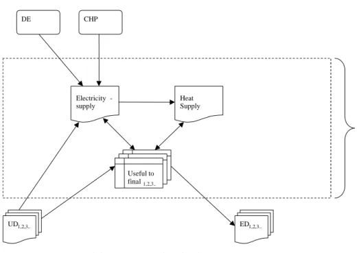
Due to the complex nature of the processes involved, supply is modelled more extensively. The process is illustrated in Figure 3.
ED1,2,3.. CHP DE UD1,2,3.. Electricity -supply Heat Supply Useful to final1,2,3..
Supply
Figure 3: Structure of the energy supply side of PIE.
Electricity supply
The ‘Electricity supply’ concerns the total electricity production and therefore includes the production which takes place at the end users.
Scaling up/down
The results from the background scenario and/or variant are used to determine how the electricity supply changes depending on alterations in the demand, manual input from the user and/or other starting points. The electricity production from natural gas acts as the balancing item for this part of the model. In other words, changes in the demand are initially translated into changes in the quantity of natural gas consumed. This factor has been introduced because many other types of capacity frequently need to be fixed in absolute terms. The principle of uniform scaling up/down of all types independent of the demand cannot meet this requirement.
Decentralised capacity
A number of capacity types can be present at the end user and, in the case of CHP (combined heat and power), can entail extra gas consumption and electricity production. This concerns large and small-scale CHP, wind power, solar power and biomass. If needed other types can be added here as well. The part of the capacity located at the end-use sectors can be entered for the capacity types concerned either by the submodel and/or the user. The sector in which the fuel consumption and the electricity production takes place is automatically calculated on the basis of the percentages entered. Conversion sector
The total electricity production is reduced by the decentralised generation. The production and capacity of the Conversion sector results from this.
Heat Supply
The heat production of the other energy sources is described under Heat Supply. The heat production concerns the production of heat combined with electricity production. This is therefore directly
linked with the electricity supply sheet. In principle, no fuel consumption is attributed to heat production. This is completely attributed to the electricity production.
Useful to Final
In ‘Useful to Final’ the distribution is once again made from the useful demand to the demand for energy carriers. In effect this is the opposite of the step from EDb to UDb.
Electricity
The category electricity under ‘Useful to Final’ is completely filled by the electricity provision; therefore the user of the model may not change the electricity part in this sheet. The extent to which the end-use sector provides for its own needs is determined on the basis of the decentralised generation and it is automatically assumed that the remaining amount is purchased from the supply sector.
Heat
There is not yet a separate submodel for the provision of the useful demand for heat by end users. Here, the user has relatively more freedom. However, a certain quantity of heat linked to the electricity production is available for heat distribution over the sectors. Further, the user of the model can fill in(if need be on the basis of submodels) whether the demand for heat is supplied by coal, oil, electricity (for example, by a heat pump) or renewable energy (solar boiler). The user should also enter the efficiencies associated with these inputs. Further, the model has been designed such that the remaining demand for heat is covered by natural gas. The calculation of the efficiency of heat production from natural gas per sector, takes into account whether the heat is produced from CHP or with a boiler. To this end, the model attributes the fuel consumption for current generation completely to electricity. This is a practical solution to ensure that the fuel consumption is not accounted for twice.
Raw material (feedstock)
The distribution of the raw materials is proportional to the distribution of raw materials in the baseline year. Therefore if only oil has been used as a raw material in the chemical industry in the baseline year, this is also the case now. However, the level of the use is adjusted depending on the volume, dematerialisation and the effects of energy savings measures.
Final balance
Eventually all of the figures are brought together in the final balance (ED1,2,3). In this balance the
demand for coal, oil, natural gas, electricity, renewable energy and other sources is stated per demanding sector. This demand must be supplied or produced by energy conversion, or by extraction or import. A negative demand from the end users means that a sector supplies this energy source to the supply sector. For example, this can happen in an industry where there is a lot of decentralised heat/power. The heat is used within the sector and the electricity is then returned to the supply net.
The data from energy conversion are also combined. In principle, coal, oil, natural gas and renewable energy are the only energy sources used per balance. In the case of electricity, this is production (and is therefore a negative number). Further, there is a balancing item which includes the production of heat, hydrogen, methanol and ethanol, but also the use of uranium and some of the waste incineration. This can therefore be both a positive as well as a negative number.
The amount of energy lost during the transport of the energy is also stated. The sum of these three categories is the total national consumption, representing the balance taken from extraction, import and export.
Emissions
The emission per unit of fuel consumed for energy at the end user is stated per energy carrier (coal, oil, natural gas, electricity, renewable, heat and other). Initially these emission factors were taken from the baseline scenario. They can be adjusted with the help of an external model.
Emissions are also released during the supply of energy. Here the emission per unit of fuel used is stated per type of conversion. Initially these were also data from the baseline scenario can be adjusted with the help of an external model.
External emission model
An accurate estimate of the emission can only be made if a model is developed in which new emission coefficients are calculated. The efficiency of the process also changes due to the range of technologies which have an effect on the emission coefficients. Therefore the efficiency is also an output of this model. For example, natural gas normally has an emission coefficient of 56.1 kg/GJinput. As part of the CO2 is stored, this coefficient will decrease, but the efficiency might
3
PIE-Excel
3.1
Introduction
This chapter contains a description of the PIE model as implemented in Excel (further referred to as: PIE-Excel). PIE-Excel is an elaboration of the theory from the previous chapters. PIE-Excel should be viewed as a working intermediate version of the final model, as described in the previous chapter. Therefore some components have still not been fully worked out as described.
PIE-Excel can be broadly divided into three blocks: i) energy demand, ii) energy supply, iii) emissions.
The calculations in the block ‘Energy demand’ proceed generally speaking as follows: first of all, the final energy demand (coal, oil, etcetera) of the end-use sectors is converted into the useful energy demand (heat, electricity and feedstock). The effects of economic changes which influence this useful energy demand are then worked out for the projected years. This provides the useful demand after energy savings measures and this useful demand is then converted into the demand for the final energy sources.
In the block ‘Energy supply’ the focus is on the origin of the useful demand from the end users. A proportion of the demand is not realised at the end user but at the central energy supply. This concerns mainly the production of electricity and heat (so-called secondary energy sources) from primary energy sources, such as coal and natural gas.
Finally, there is the block ‘Emissions’. Here, the emissions from both the end user sectors and the energy production sector are calculated.
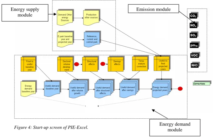
These sheets correspond with the different blocks in the start-up screen of PIE-Excel. This screen is shown in Figure 4.
Figure 4: Start-up screen of PIE-Excel.
By clicking on the coloured blocks, a sheet with the corresponding information will be displayed. Some data need to be entered whereas other data are the results of calculations. In PIE-Excel the cells for data to be entered are marked in yellow.
3.2
Energy demand from end-use sectors
3.2.1 Introduction
Table 2 shows the classification chosen for the end-use sector in PIE-Excel.
Energy demand module Energy supply
module
Table 2: End-use sectors in PIE
Sector Subsector
Industry Food
Chemical
Primary metals industry Other metal industries Construction materials Printing and paper Refineries Other industry Agriculture Horticulture Other agriculture Transport People Goods
Services Trade and catering Business services Non-profit sector Households New buildings
Existing buildings Appliances
The energy demand for these sectors is determined by the input of variables and calculations in the following sheets:
• ‘EdB’: final energy demand for baseline year;
• ‘final to useful’: conversion final energy demand into useful energy demand; • ‘UdB’: useful energy demand for baseline year;
• ‘volume’: the volume effects for the projected years; • ‘UDafterV’: useful energy demand after volume growth;
• ‘dematerialisation’: the structural effects for the projected years; • ‘UDafterD’: useful energy demand after the structural effects; • ‘savings’: the savings measures for the projected years;
• ‘temperature correction effect’: the temperature corrections for the projected years; • ‘UDafterC’: useful energy demand after energy savings measures;
• ‘Useful to Final’: conversion of useful energy demand to final energy demand; • ‘ED’: conversion of useful energy demand to final energy demand.
The necessary inputs and the calculations in these sheets are explained in the following subsections.
3.2.2 ‘EdB’: Final energy demand for baseline year
In this first sheet EdB (EnergyDemandBaseline year) the final demand for energy sources per end-use sector is given for the baseline year. This final energy demand is subdivided into:
• coal • oil • natural gas • electricity • renewable • heat • other
This sheet serves as the basis for all other calculations. No further calculations are carried out in EdB.
3.2.3 ‘FinaltoUseful’: conversion of final energy demand into useful energy
demand
The aforementioned energy sources are in many cases converted into so-called ‘useful energy sources’. In PIE-Excel the following useful energy sources are distinguished:
• heat • electricity
• feedstock (raw materials for chemical products)
The following variables are needed for the translation from final energy sources to useful energy sources (see also the Appendix):
• Which part of the final energy demand from sheet EdB is used as feedstock? (feedstock contribution)
• The efficiency (% of the energy content for energetic purposes) with which the final energy sources are converted into useful energy sources (efficiency of UdB).
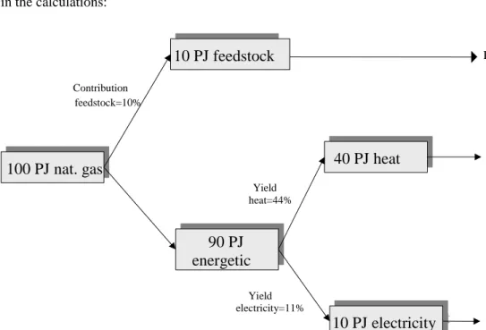
Figure 5 illustrates how the contribution feedstock and the heat and electricity efficiencies are used in the calculations:
Figure 5: Scheme showing Final to Useful.
100 PJ aardgas
100 PJ nat. gas
10 PJ feedstock
10 PJ feedstock
40 PJ warmte
40 PJ heat
90 PJ
energetisch
90 PJ
energetic
10 PJ elektriciteit
10 PJ electricity
Contribution feedstock=10% Yield heat=44% Yield electricity=11% Electricity 10 PJ Heat 40 PJ Feedstock 10 PJ
The total demand per subsector for heat, electricity and feedstock is calculated by repeating this process for each final energy source.
3.2.4 ‘UdB’: useful Energy demand baseline year
The results from the ‘Final to Useful’ sheet are calculated in the ‘UdB’ sheet and summed for the three secondary energy sources: heat, electricity and feedstock.
Example: The chemical sector uses 100 PJ oil and 200 PJ coal as EdB; 70% of the coal is used as feedstock (feedstock contribution); 10% of the energy content becomes electricity and 5% heat. The remaining 15% is lost, while 60% of the oil is used for electricity and 10% for heat.
Table 3 shows what the useful demand of the chemical sector will therefore be.
Table 3: Exemplary calculation of Useful demand
From coal From oil UdB
Feedstock 0.7*200 - 140
Heat (1-0.7)*200*0.05 100*0.1 13
Electricity (1-0.7)*200*0.1 100*0.6 12
3.2.5 ‘Volume’: the volume effects for the projected years
The demand for useful energy from the ‘UdB’ sheet is used as the basis for the calculation of the demand for useful energy carrier in the projected years. The first step in this process is to calculate the energy demand in the projected year, if the useful demand in each subsector grows at the same rate as the Monetary Added Value of this sector (the so-called volume effect).
The ‘volume’ sheet contains the annual growth percentages of the added value per subsector. These are expressed in blocks up to and including each projected year to be calculated.
3.2.6 ‘UDafterV’: useful Energy demand after volume growth
UDafterV is the useful demand after volume growth, and is the useful energy demand after the volume growth from the ‘volume’ sheet.
with
UDafterVi,j Useful Demand after Volume growth for end-use sector i and useful
energy source j.
UdBi,j Useful Demand Baseline year for end-use sector i and useful energy source
j.
volume growthi volume growth for end-use sector i and useful energy source j
3.2.7 ‘Dematerialisation’: the structural effects for the projected years
The next step in calculating the useful demand in the projected year is the calculation of the energy demand after volume growth and dematerialisation.
In the sheet ‘dematerialisation’ the percentage by which the volume growth must be reduced annually to calculate UDafterD (Useful Demand after Dematerialisation) is stated for the projected years per subsector and per useful energy source.
3.2.8 ‘UDafterD’: useful Energy demand after structural effects
The equation to calculate the useful energy demand after dematerialisation (UDafterD) from the useful demand after volume growth (UDafterV) for end-use sector i and energy source j in a given projected year t is then:
where:
UDafterDi,j Useful Demand after Dematerialisation for end-use sector i and useful
energy source j.
UDafterVi,j Useful Demand after Volume growth for end-use sector i and useful
energy source j.
dematerialisationi,j annual percentage change in the volume growth for end-use sector i and
useful energy source j.
3.2.9 ‘Temperature correction effect’: the temperature corrections for the
projected years.
Over the past 10 to 15 years it has gradually become warmer in the Netherlands during both the summer and the winter. This trend is expected to continue. This has a more than negligible effect on energy use, particularly for heating buildings in the winter, which is taken into consideration in the projections of the energy use by correcting the useful demand for energy for the expected number of heating degree days.
3.2.10 ‘Savings’: the energy savings measures for the projected years
The last step in calculating the useful demand in the projected year is the calculation of the energy demand after volume growth, and after dematerialisation and savings measures.
In the ‘Conservation’ sheet the percentage by which the volume growth must be reduced annually to calculate the UDafterC (Useful Demand after Conservation) is stated for the projected years per subsector and per useful energy source.
3.2.11 ‘UDafterS’: Useful energy Demand after Savings
where:
UDafterCi,j Useful Demand after Savings for end-use sector i and useful energy source
j.
UDafterDi,j Useful Demand after Dematerialisation for end-use sector i and useful
energy source j.
(2)
UDafterD
i,j=
UDafterV
i,j*
(
1
+
dematerial
isation
i,j)
t(3)
i j t j i j i j iUDafterD
savings
C
UDafterS
,=
,*
(
1
+
,)
*
,
savingsi annual percentage change in the growth after dematerialisation for end-use
sector i and useful energy source j.
Ci,j Temperature correction
3.2.12 ‘Useful to Final’: conversion of Useful energy demand to Final energy
demand
The data to convert the useful energy demand for a projected year back into a final energy demand are entered on this sheet. This is the reverse step to the step taken in ‘Final to Useful’. The following data are necessary for this calculation:
- The contribution of the useful energy source produced by the Final Energy sources;
- The efficiency of the production of Useful energy sources from the final energy sources (for example, how many units of coal are needed to produce one unit of heat?).
The boiler efficiency is also entered on this sheet, as explained in Chapter 3.4.
3.2.13 ‘ED’: conversion of useful energy demand to final energy demand
The ‘Useful to Final’ and ‘UDafterC’ sheets are now combined to create the Final energy demand for Projected year (ED).
For sector i, the useful energy demand source after savings k is converted into the final energy demand source j, using:
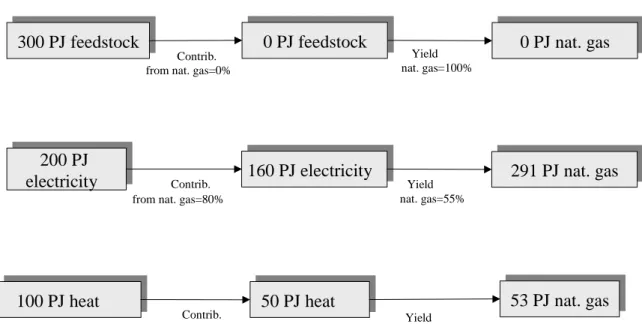
Figure 6 illustrates how the final demand for natural gas, for example, is calculated. In this example the final natural gas demand is therefore 344 PJ. In effect this is the reverse scheme of Figure 1 in Chapter 2.
(4)
=
∑
k j iUDafterC
ED
k j, i, k i, k j, i, ,efficiency
*
on
contributi
200 PJ
elektriciteit
200 PJ
electricity
300 PJ feedstock
300 PJ feedstock
50 PJ warmte
50 PJ heat
Contrib. from nat. gas=50%Useful Demand
100 PJ warmte
100 PJ heat
160 PJ elektriciteit
160 PJ electricity
Contrib. from nat. gas=80%0 PJ feedstock
0 PJ feedstock
Contrib. from nat. gas=0%
53 PJ aardgas
53 PJ nat. gas
Yield nat. gas=95%291 PJ aardgas
291 PJ nat. gas
Yield nat. gas=55%0 PJ aardgas
0 PJ nat. gas
Yield nat. gas=100% Final DemandFigure 6: Example ‘Useful to Final’ for natural gas
3.3
Energy supply Conversion sector
3.3.1 Introduction
The demand for the final energy carriers is calculated in the block ‘Energy demand’. A number of these energy carriers, e.g. electricity, are produced from other energy carriers (coal, natural gas, biomass, wind, etcetera). This production takes place in a separate Conversion sector but can also take place in the end-use sector. This section describes the block ‘Energy supply’, where the production of the energy carriers in the Conversion sector is modelled. The following section details the interaction with the production that takes place in the end-use sectors. The ‘Electricity supply’ sheet is now described. The electricity production park is first described ; this is flowed by the calculation of the use of energy. Finally, the ‘Demand other’ sheet describes the demand for other (non-electrical) energy sources, which are produced centrally. The heat production in the electricity supply is also considered under this sheet.
3.3.2 ‘Electricity supply': data on the electricity production park
In the ‘Electricity supply’ sheet data are entered for the total electricity production park (further referred to as ‘park’) as below:
1. production data for the park;
2. distribution of decentralised production over the subsectors;
Production data for the par;
In this model it is assumed that the park consists of the following types of plants:
• Natural gas • Solar
• Coal • Waste incineration plants
• Nuclear • Biomass
• Oil • Other
• CHP (Warmth Distribution) • Import
• CHP−large • Gas + CO2
• CHP−small • Coal + CO2
• Wind
The following characteristics are entered for each type: • Electrical capacity (in MW);
• Operational time per power station (in hours); • Electrical efficiency (%);
• Thermal efficiency (%).
The aforementioned characteristics are entered for both the plants in existence since the baseline year (baseline park) and those which have been built since (new capacity). These need to be entered separately because new plants often have production characteristics differing from the ’old’ plants. For example, an entry stating:
baseline year, existing capacity (MW)
Type 2000 2010
natural gas 1000 500
new, capacity currently under construction (MW)
Type 2000 2010
natural gas 0 1000
means that in 2010 there are still 500 MW of plants from the year 2000 running on natural gas, and that an additional 1000 MW have been constructed up to 2010.
Distribution of decentralised production over the subsectors Several types of plants are set up to run at end users. These are: • CHP−large
• CHP−small • Solar • Wind • Biomass
In the ‘Electricity supply’ sheet it must be stated that the production from these plants is distributed over the subsectors, being necessary for the calculations in Chapter 3.3.
Consumption balance of the final energy sources from the distribution sector
3.3.3 ‘ref, act, conv’: calculation of the reference, current and central parks
Reference park
The following are calculated per type of plant using the capacity, operational time and electrical and thermal efficiencies entered on the ‘Electricity supply’ sheet:
• Electricity production (in PJ) • Fuel consumption (in PJ) • Heat production (in PJ) by using the following formulae:
(5)
610
3.6
*
time
l
operationa
*
capacity
Electrical
production
-E
=
(6)
efficiency
Elektrical
production
-E
n
Consumptio
Fuel
=
(7)
Heat
-
production
=
Fuel
consumptio
n
*
Thermal
efficiency
The reference park is calculated by adding up the fuel consumption and heat production of the ‘park Baseline year’ and ‘park New capacity’ per year and per power station type.
Current park
The adjustments for a scenario can be such that the production of the Reference park no longer relates to the new electricity demand (as calculated in Chapter 3.2.11).
If this is the case, the electricity production from natural gas is used as the balancing correction. In other words a greater or lesser demand is translated into a greater or lesser natural gas burning capacity. This factor has been introduced due to the frequent requirement to fix other types of capacity in absolute terms. The principle of uniform scaling up/down of all types dependent on demand cannot be used in this case.
Natural gas as a balancing correction is calculated as follows:
First of all the total electricity demand is determined. This is the sum of the electricity demand of end users, on the one hand, and the electricity demand of the distribution companies, on the other. The electricity demand of the end users is calculated as the sum of:
1. the useful electricity demand after electricity savings (UDafterC, see Chapter 3.2.11); 2. the electricity needed for the production of heat (e.g. electricity for electric heaters); 3. the electricity needed for feedstock (e.g. electricity for electrolysis).
Expressed in an equation form this is per subsector:
feedstock to elec. conversion production feedstock in elec. feedstock heat to elec. conversion production heat in elec. heat elek efficiency on Contributi * UDafterC efficiency on Contributi * UDafterC UDafterC ElekDemand Totale = + +
The second part of the equation can be described as the part of the total demand for heat that is generated with electricity (above the dividing line) divided by the efficiency of this conversion. The third part of the equation is then the part of the total demand for feedstocks produced using electricity (above the dividing line) divided by the efficiency of this conversion.
The electricity demand for each subsector is calculated as such and then summed; the electricity demand of the distribution sector is added to this to give the total electricity demand.
The plant type ‘natural gas’ is then corrected for to satisfy this demand. The park calculated in this case is the Current Park.
Park Conversion sector
As previously stated not all of the plants are located in the Conversion sector; in fact, a certain percentage of the following are found in the end-use sectors:
• CHP–large • CHP–small • Wind • Solar • Biomass
The ‘Electricity supply’ sheet states the proportion located in the end-use sectors. The composition of the Conversion sector’s production can be calculated by correcting the current park with these percentages.
The Conversion sector has to transport the electricity over considerable distances, which leads to losses during transport. Therefore in practice more must be produced than is demanded by the end users. These transport losses are stated in the ‘Useful to Final’ sheet. The ‘park Conversion sector’ is calculated by correcting for this.
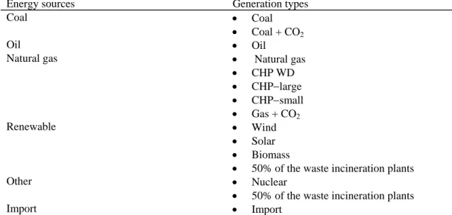
Distribution over the energy sources
The fuel consumption of the different types of generation in the Conversion sector is distributed over the energy sources: coal, oil, natural gas, electricity, renewable, other and import. This is done in accordance with the following distribution:
Table 4: Distribution of the final energy sources over the various generation types
Energy sources Generation types
Coal • Coal
• Coal + CO2
Oil • Oil
Natural gas • Natural gas
• CHP WD • CHP−large • CHP−small • Gas + CO2 Renewable • Wind • Solar • Biomass
• 50% of the waste incineration plants
Other • Nuclear
• 50% of the waste incineration plants
Import • Import
3.3.4 ‘Demand other’: demand on other energy sources by the end users
In addition to electricity the Conversion sector also produces heat. This heat production is calculated in the sheet: ‘ref, act, conv’. Which part of this production is supplied to various end-use sectors is described in the ‘Demand other’ sheet, which also contains the efficiency of transporting heat. The demand for other energy sources can also be entered here.
3.4
Linking supply to demand: ‘Useful to Final’ sheet
As previously described, the sheet ‘Useful to Final’ is intended to convert the useful energy demand from the end-use sectors in a projected year back into the final energy demand. This is the reverse step of ‘Final to Useful’. The following data are needed for this calculation (Chapter 3.2.12):
- The proportion of the useful energy source produced by the final energy sources;
- The efficiency of the production of useful energy sources from the final energy sources (for example, how many units of coal are needed to produce one unit of heat).
However, not everything from this sheet is input. Since how much of the park is located at the end-use sectors is also calculated in the ‘ref, act, conv’ sheer, this must also be corrected for in the ‘Useful to Final’ sheet. This ensures that in the model the end-use sectors do not produce more or less electricity than that calculated in ‘ref, act, conv’.
Table 5: Exemplary table Useful to Final
The calculations pertaining to the circled numbers are explained in the following subsections. Point 1: Efficiency of heat generation with natural gas.
In a developmental version of PIE, the following was determined about the method of calculating the efficiency of heat generation using natural gas:
‘The calculation of the efficiency of heat production from natural gas per sector takes into account whether the heat is produced from CHP and/or a boiler. Here, the fuel consumption from the current generation is completely ascribed to electricity.’ This should be borne in mind.
Efficiency is calculated by dividing the quantity of heat that comes OUT of the plant by the total amount of energy that goes IN to the plant.
However, here we are concerned with two systems for producing heat: the CHP plant production and the conventional heat production from a boiler. The efficiency in sector i for heat in a given projected year is then simply calculated as follows:
1
2
3
4
5
7
6
The gas input for the boilers is calculated by dividing the quantity of heat emitted from the boiler by the boiler efficiency. The boiler efficiency is entered in ‘Useful to Final’.
The gas input for the CHP plant is ascribed to electricity production (point to remember) and therefore the gas input for CHP is, by definition, 0.
i i i i gas natural i,
efficiency
boiler
boiler
production
heat
0
boiler
production
heat
CHP
production
heat
rendement
+
+
=
The quantity of heat produced by the boiler (heat production boileri), is calculated as follows:
First of all the total amount of heat produced using natural gas (therefore the boiler and CHP combined) is determined by multiplying the contribution of natural gas in heat production by the total demand for heat (UDafterCheat). The heat production from CHP is obtained as such.
The resulting equation is then (enter heat production boileri):
i i heat i i heat i i gas natural i,
efficiency
boiler
CHP
production
heat
-UDafterC
*
on
contributi
)
CHP
production
heat
-UDafterC
*
ion
(contribut
CHP
production
heat
efficiency
=
+
This can be rewritten as:
i heat i heat i i gas natural i,
CHP
production
heat
-UDafterC
*
on
contributi
UDafterC
*
on
contributi
*
efficiency
boiler
efficiency
=
The two variables to be filled in, i.e. contributioni and heat production CHPi are explained in point 4
and the following section, respectively.
(8)
i i i i gas natural i,boiler
input
gas
CHP
input
gas
boiler
production
heat
CHP
production
heat
efficiency
+
+
=
(9)
⎟⎟
⎠
⎞
⎜⎜
⎝
⎛
=
heat i i i i gas natural i,UDafterC
CHP
production
heat
-on
contributi
efficiency
boiler
*
on
contributi
efficiency
CHP heat production
The CHP heat production is divided up within PIE into the production from large plants (CHP– large) and the production from small plants (CHP–small). These plants can be located in both the end-use sectors and the Conversion sector. In PIE-Excel, which proportion of the CHP production taking place in which end-use sector must be entered on the ‘Electricity supply’ sheet.
The aforementioned percentages must be multiplied by the total CHP production in order to calculate the total CHP heat production per sector. In PIE the total heat production is calculated separately and further explained in Section 3.3.3.
Point 2: efficiency electricity generation using natural gas.
In PIE it is assumed that the natural gas consumption for CHP plants is completely ascribed to electricity. The two types of CHP plant, CHP–large and CHP–small, are used in the following equation i to calculate the electrical efficiency for sector i:
i i i i i
in)
large
-(CHP
in)
small
-(CHP
out)
large
-(CHP
out)
small
-(CHP
:
efficiency
+
+
If it is assumed that the plants in each sector have the same efficiency, the efficiency for sector i is described as: ⎟⎟ ⎠ ⎞ ⎜⎜ ⎝ ⎛ + ⎟⎟ ⎠ ⎞ ⎜⎜ ⎝ ⎛ + = large CHP efficiency out) large CHP ( * on contributi small CHP efficiency out) small (CHP * on contributi out) large CHP ( * on contributi out) small (CHP * on contributi efficiency total i large, -CHP total i small, -CHP total i large, -CHP total i small, -CHP i
This is in effect a sort of average efficiency for CHP–large and CHP–small. Point 3: efficiency electricity generation with renewable resources.
The electricity produced from renewable energy (solar, wind and biomass) is divided by the quantity of energy needed to generate this. The quantity of energy needed for the generation, is, just as in point 2, calculated by dividing the electricity produced by the efficiency. This provides a sort of weighted average of the efficiency from renewable sources.
Point 4: proportion of heat generation with natural gas This balancing item is calculated as:
Contributionnatural gas=1 - contributioncoal – contribution oil – contributionelectricity – contributionsustainable - contributionother
For the traffic sector, oil is the balancing item.
Point 5: The proportion of Other in the heat production
This item ‘other’ is calculated by dividing the heat production for energy from other heat sources by the total quantity of heat produced. Expressed as:
heat i, heat i, i i UDafterC efficiency * supply other by supplied demand heat * supply other heat to on contributi other on contributi =
The ‘heat demand supplied by other' is the total heat production from the sheet on ‘Supply other’ divided by the Transport efficiency for heat from the sheet ‘Demand other’. The efficiencyi,heat also
comes from the ‘Useful to Final’ sheet.
Point 6: The proportion of natural gas and renewable energy in the electricity production natural gas
Natural gas
It is once again assumed that in the end-use sectors all of the electricity production in CHP plants takes place with natural gas as the raw material. The proportion is then calculated by dividing the electricity production from CHP plants by the total electricity demand. As previously stated there are small and large CHP plants.
The ‘Electricity supply’ sheet states what part of the capacity from the two different types of CHP plants is located in what sectors (see 0). Using this and the total electricity production from the two different types of CHP plants (also calculated in the sheet ‘Electricity supply’), the electricity generated by each type of CHP plant in the sectors concerned can also be calculated. The proportion of natural gas in the electricity production in sector i is therefore calculated as:
i i i i demand y electricit Total large CHP production total * groot CHP on contributi small CHP production total * small CHP on contributi gas nat. on contributi = + Renewable energy
The calculation of the proportion of renewable energy in electricity generation per sector is analogous to that of natural gas. Instead of two types (CHP–small and CHP–large), three types can be distinguished for electricity generation using renewable sources: wind, solar and biomass. Point 7: proportion of electricity in electricity generation.
The difference in amount between the electricity demand and electricity supply within a sector is purchased (in other words, what the sector cannot produce itself is purchased). The proportion of this purchased electricity is therefore a balancing item calculated as:
Contributioni=1-contribution nat. gasi – contribution renewablei – contribution coali – contribution oili – contribution otheri
Assumptions:
- No feedstock contribution from 'other';
- No decentralised electricity generation from coal, oil and other; - Efficiency of electricity from electricity is always 100%.
3.5
Emissions from the Conversion sector
3.5.1 ‘EmConv’: emission factors and emissions from the Conversion sector
Emissions from electricity production
For the calculation of the emissions from the electricity production the emission factors per substance and the plant type must be entered in the ‘EmConv’ sheet for both the Existing Park and the New Park. The emissions are calculated in the following order: reference park, current park and conversion park. The emissions from the reference park are determined by multiplying the fuel consumption of the existing park, calculated in the sheet 'Electricity supply', by the emission factors of the existing park, and adding this to the fuel consumption of the new park multiplied by the emission factors of the new park. Then the emissions of the current park are calculated by correcting the reference park for the greater or lesser consumption of natural gas. Finally, the emissions of
conversion park are calculated by multiplying the emissions from the current park by the proportion of the Conversion sector in the production as stated in the ‘Electricity supply’ sheet.
Comments
• For the CO2 emission of waste incineration plants it is assumed that half of this is short-cycle
and therefore does not need to be considered as harmful emission. This is corrected for by introducing a waste incineration plant correction factor.
Emissions from transport/distribution
As the transport/distribution sector also falls under the energy companies, the emission calculations of this sector are included in ‘EmConv’. Emission factors are entered for each energy source and year; subsequently, the emissions of this sector are determined.
3.6
Emissions from the end-use sectors
3.6.1 Introduction
The emission calculations of the end-use sectors have not been placed in a single sheet because the emission factors must be entered for each substance and emissions are calculated per projected year, per sector, per energetic, process or feedstock emission, and per final energy source. This means, for example, that for 10 sectors, 3 years, 6 energy sources and 5 substances, there are about 3800 items of data. A single sheet containing all of this information would be too large and unwieldy to use. Therefore there are two sheets for each substance: ‘Emission factor Compound X’ and ‘Emission Compound X’.
3.6.2 ‘Emission factor Compound X’
In this sheet the following three variables are entered per projected year and per sector:
1. Energetic emission factors per final energy source for the calculation of the emissions from energetic applications;
2. Feedstock fixed percentage per final energy source for the calculation of the feedstock emissions (only for CO2);
3. Process emissions.
These three variables are then used to calculate:
- The emissions from energetic applications by multiplying the emission factors from point 1) by the consumption balances from the sheet ‘ED’.
- The feedstock emissions per sector, final energy source and projected year, which takes place as follows:
(
1
fixed
percentage
)
*
feedstock
use
*
emission
factor
feedstock
=
−
Putting this into words then: a certain part of the feedstock use from the sheet ‘ED’ is not permanently fixed, but the carbon in this is eventually released back into the atmosphere
(1-feedstock fixed percentage)*feedstock use. The quantity of carbon released is assumed to be equivalent to the quantity that would have been released had it been combusted (therefore: *emission factor).
3.6.3 ‘Emission Compound X’
In the ‘Emission’ sheet the emissions are summed and presented per main sector and per projected year. For the sake of completeness the emissions from the energy sector are also presented here.
4
Conclusions and follow-up
This report, forming an element of the PIE joint project of ECN and MNP, has provided a description of the PIE information system and its application. The chosen structure explained here seems to satisfy the stated objectives. The next step is to apply the PIE information system. The following actions will be undertaken in the short term in order to realise this:
1. A protocol and transfer module will be developed to transfer the energy data from ECN into PIE;
2. The results of projections currently developed in the Reference framework energy and emissions, and the scenarios from the Welfare and Living Environment project (Dutch acronym: WLO), will be implemented in PIE using the transfer module.
List of tables and figures
Tables
Table 1: End-use sectors of PIE...14
Table 2: End-use sectors in PIE ...21
Table 3: Exemplary calculation of Useful demand...23
Table 4: Distribution of the final energy sources over the various generation types ...30
Table 5: Exemplary table Useful to Final ...31
Figures Figure 1: Structure of the Platform on Integral Energy and emission projections...10
Figure 2: Structure of the energy demand side of PIE. ...13
Figure 3: Structure of the energy supply side of PIE. ...16
Figure 4: Start-up screen of PIE-Excel. ...20
Figure 5: Scheme showing Final to Useful. ...22
Reference
Appendix A
Definition efficiencies in PIE
This appendix describes the definition of efficiencies in PIE using a numerical example. In a number of cases the definition in combination with the lack of certain data can result in deviant values for historical years. This does not have any consequences for the utility of PIE, since the definition always concerns values of arithmetic efficiencies, which indicate the relationship between fuel consumption and the production of heat and electricity. However, the values from this are correct at the aggregated levels.
Streams and processes
The diagram shows an example of streams and efficiencies in the case where everything is known at the level of streams and processes. The figures have been chosen such that no single figure occurs twice. All of the efficiencies and streams are at process level. For CHP the efficiency of the total input is used to calculate both heat and electricity; the input is not differentiated into a part for heat and a part for electricity. This information is not available at this detailed level in PIE. Therefore PIE has to calculate using overall efficiencies for ‘Useful to Final' and 'Final to Useful’.
The following figures show the calculated efficiencies for ‘Final to Useful’ and ‘Useful to Final’. As in the following diagrams, the separate processes are no longer known; the efficiencies deviate from the efficiencies shown here, although the underlying system is identical.