Dioxins in Dutch vegetables

(1)

RIVM report 310305003/2004

Dioxins in Dutch Vegetables

R Hoogerbrugge, MI Bakker, WC Hijman, ACdenBoer, RS den Hartog, RA Baumann

With the cooperation of: G Groenemeijer B Stoffelsen R Zwartjes D Mooibroek R van Poll J Freijer H Bremmer G ten Hove

This investigation has been performed by order and for the account of the Inspectorate for Health Protection and Veterinary Public Health, within the framework of project 310305: Dioxins in food.

(2)

Abstract

The exposure to dioxins (including polychlorinated dibenzo-p-dioxins, dibenzofurans and dioxin-like polychlorinated biphenyls) occurs predominantly via the intake of food. The main contribution to the total intake originates from the consumption of animal fat. Nevertheless, vegetables were estimated to contribute 13 % to the total dietary intake, although the uncertainty in this figure was considered large in a previous investigation. In the present study, a detailed investigation into the concentrations of dioxins in vegetables and subsequently the intake via the consumption of vegetables is calculated. To that aim, eighteen different vegetables were purchased in eight Dutch retail shops in two different seasons. The samples were pooled per season and analysed for dioxins. The summer vegetables could be measured very sensitively: the maximum levels (assuming that samples below the limit of detection -LOD- equal a concentration equal to the LOD) vary between 3 and 10 pg toxic equivalents (TEQ) per kg fresh weight (FW). The winter vegetables could be measured less sensitively; the LOD for each congener was approximately 10 pg TEQ/kg FW. The maximum levels (with the exception of curly kale) vary between 30 and 70 pg TEQ/kg FW. The average level in curly kale is estimated as 100-200 pg TEQ/ kg FW. Using the maximum levels, the average intake of dioxins, furans and dioxin-like PCBs

by the consumption of vegetables is estimated as 0.12 pg TEQ/kg

bodyweight/day. When a consistency of patterns between detected and non-detected levels is assumed, the most likely estimate is 0.014 pg TEQ/ kg bodyweight/day, with an estimated standard deviation of 0.003 pg/kg bw/day. Using this most likely estimate, the calculated intake of dioxins by the consumption of vegetables contributes less than 2 % to the mean daily intake from the total diet. Therefore, the vegetable related exposure to dioxins is (almost) negligible compared to other food categories, such as meat products, fish and dairy.

(3)

Samenvatting

De blootstelling aan dioxinen vindt voornamelijk plaats via de voeding. De belangrijkste bron van deze stoffen in de voeding is dierlijk vet. Desalniettemin is de bijdrage van groenten geschat op 13 % van de totale dioxine-inname via de voeding, hoewel de onzekerheid van die waarde groot werd geacht (Freijer et al., 2001). Het doel van de huidige studie is om de dioxineconcentraties in individuele groenten en vervolgens de inname door de consumptie van groenten vast te stellen. Daartoe zijn achttien soorten groenten ingekocht bij acht Nederlandse detailhandels in twee seizoenen. De monsters zijn per seizoen gemengd en geanalyseerd op het vóórkomen van polychloordibenzo-p-dioxinen en -dibenzofuranen (PCDDs/PCDFs) en de dioxine-achtige non-ortho polychloorbifenylen (no-PCBs). De bijdrage aan de toxiciteit van de PCDDs/PCDFs was in het algemeen veel groter dan die afkomstig van de no-PCBs, derhalve werd de analyse van de overige dioxineachtige (mono-ortho) PCBs niet noodzakelijk geacht.

De zomergroenten zijn met extreme gevoeligheid geanalyseerd. De maximum niveaus (waarbij als een congeneer niet werd aangetroffen de concentratie werd aangenomen ter waarde van de detectielimiet) variëren van 3 tot 10 pg toxische equivalenten (TEQ) per kg versgewicht.

De analyse van de wintergroenten was iets minder gevoelig. Hierbij zijn detectiegrenzen gehaald van ongeveer 10 pg TEQ/kg versgewicht per congeneer. De maximum niveaus (met uitzondering van boerenkool) variëren van

30 -70 pg TEQ/kg versgewicht. Het gemiddelde niveau van de boerenkool is

100-200 pg /kg versgewicht.

Met deze maximale niveaus kan een maximale gemiddelde inname via de consumptie van groente van 0,12 pg TEQ/kg lichaamsgewicht/dag worden geschat. Indien wordt aangenomen dat er een consistent patroon is voor deze verbindingen in de diverse typen groenten dan is de meest waarschijnlijke gemiddelde inname ongeveer 0,014 pg TEQ/kg lichaamsgewicht/dag, (met een geschatte standaarddeviatie van 0,003 pg TEQ/kg lichaamsgewicht/dag). De inname van dioxines via de consumptie van groenten berekend met deze waarde bedraagt minder dan 2 % van de totale gemiddelde dioxine inname. De blootstelling aan dioxinen via groenten is dus (bijna) verwaarloosbaar vergeleken met andere voedselcategorieën (zoals vlees, vis en zuivel).

(5)

Summary

The exposure to dioxins occurs predominantly via the intake of food. The main contribution to the total intake originates from the consumption of animal fat. Nevertheless, vegetables were estimated to contribute 13 % of the total dietary intake. although the uncertainty was large (Freijer et al., 2001). In the present study, a detailed investigation into the concentrations of dioxins in vegetables and consequently, into the intake via the consumption of vegetables, is carried out. To this aim, eighteen different vegetables were purchased in eight Dutch retail shops in two different seasons. The samples were pooled per season and analysed for polychlorinated dibenzo-p-dioxins and dibenzofurans (PCDD/Fs) and the dioxin-like non-ortho polychlorinated biphenyls (no-PCBs). The contribution to the toxicity was much larger for the PCDD/Fs than for the no-PCBs, therefore the analysis of the other dioxin-like (mono-ortho) PCBs was considered not necessary.

The summer vegetables could be measured very sensitively: the maximum levels (assuming that samples below the limit of detection -LOD- equal a concentration equal to the LOD) vary between 3 and 10 pg toxic equivalents (TEQ) per kg fresh weight (FW). The winter vegetables could be measured less sensitively; the LOD for each congener was approximately 10 pg TEQ/kg FW. The maximum levels (with exception of curly kale) vary between 30 and 70 pg TEQ/kg FW. The average level in curly kale is estimated as 100-200 pg TEQ/ kg FW.

Using the maximum levels, the average intake of dioxins, furans and dioxin-like PCBs by the consumption of vegetables is estimated as 0.12 pg TEQ/kg bodyweight/day. When a consistency of patterns between detected and non-detected levels is assumed, the most likely estimate is

0.014 pg TEQ/kg bodyweight/day, with an estimated standard deviation of

0.003 pg TEQ/kg body weight/day. The most likely intake is less than 2 % of the mean daily intake from the total diet. Therefore, the vegetable related exposure to dioxins is (almost) negligible compared to other food categories, such as meat products, fish and dairy.

(6)

1. Introduction

In the past decade there has been much attention for the presence of organic micropollutants such as polychlorobiphenyls (PCBs), polychlorinated dibenzo-p-dioxins (PCDDs) and dibenzofurans (PCDFs) in the diet. This interest has started, in the Netherlands, in the eighties of the previous century with the contamination of cow’s milk with PCDDs originating from a municipal waste incinerator. Concentrations of these substances in the diet have declined since, but are presently strictly monitored. In a recent study the median dietary intake of PCDD/Fs and dioxin-like PCBs in the Netherlands during a human life was calculated to be 1.2 pg WHO-TEQ/kg bw/day (Freijer et al., 2001; Baars et al., 2004). In comparison, the TDI derived by the Scientific Committee on Food is 2 pg WHO-TEQ/kg bw/day. In the study of Freijer et al. (2001) the intake of dioxins due to the consumption of vegetables was estimated at 13 % of the total intake. Freijer et al. used a composite sample that contained a proportion of the vegetables as consumed in the Netherlands. Mainly because of low levels of dioxins in vegetables the determination of the average level in this composite sample was difficult, which resulted in an estimate with substantial uncertainty. This uncertainty is rather important in the subsequent dioxin intake calculation because of the large consumption of vegetables and of the decreasing levels in other food stuffs. Therefore the present study was conducted, based on composite samples for all relevant types of vegetables instead of on a single composite sample.

(7)

2. Vegetable selection and sampling

2.1 Selection of vegetables

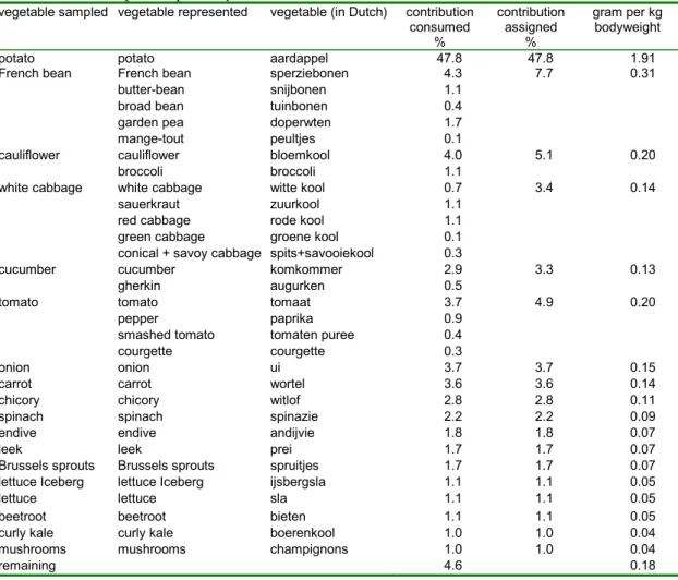
Based on the consumption pattern of vegetables in the Netherlands the eighteen most important vegetables were selected using the Dutch National Food Consumption Survey 1998 (DNFCS 3, Kistemaker et al., 1998). For some other vegetables the characteristic properties (leaf surface with respect to the weight, growing period, existence of the edible part below or above the surface etc.) were assumed to be sufficiently comparable to estimate the concentration of dioxins by its look-a-like. For example broccoli is estimated by cauliflower and red cabbage by white cabbage. The vegetables, the portion of Dutch consumption and the contribution by look-a-likes are summarized in Table 1.

Table 1. Estimated average intake of vegetables by the Dutch population. Both in gram vegetable per kg bodyweight per day and as percentages. Also the assignment of vegetables that were not sampled explicitely to the best look-a-like are shown. See also the text.

vegetable sampled vegetable represented vegetable (in Dutch) contribution consumed % contribution assigned % gram per kg bodyweight

potato potato aardappel 47.8 47.8 1.91

French bean sperziebonen 4.3

butter-bean snijbonen 1.1

broad bean tuinbonen 0.4

garden pea doperwten 1.7

French bean mange-tout peultjes 0.1 7.7 0.31 cauliflower bloemkool 4.0 cauliflower broccoli broccoli 1.1 5.1 0.20

white cabbage witte kool 0.7

sauerkraut zuurkool 1.1

red cabbage rode kool 1.1

green cabbage groene kool 0.1

white cabbage

conical + savoy cabbage spits+savooiekool 0.3

3.4 0.14 cucumber komkommer 2.9 cucumber gherkin augurken 0.5 3.3 0.13 tomato tomaat 3.7 pepper paprika 0.9

smashed tomato tomaten puree 0.4

tomato

courgette courgette 0.3

4.9 0.20

onion onion ui 3.7 3.7 0.15

carrot carrot wortel 3.6 3.6 0.14

chicory chicory witlof 2.8 2.8 0.11

spinach spinach spinazie 2.2 2.2 0.09

endive endive andijvie 1.8 1.8 0.07

leek leek prei 1.7 1.7 0.07

Brussels sprouts Brussels sprouts spruitjes 1.7 1.7 0.07

lettuce Iceberg lettuce Iceberg ijsbergsla 1.1 1.1 0.05

lettuce lettuce sla 1.1 1.1 0.05

beetroot beetroot bieten 1.1 1.1 0.05

curly kale curly kale boerenkool 1.0 1.0 0.04

mushrooms mushrooms champignons 1.0 1.0 0.04

(8)

2.2 Sampling

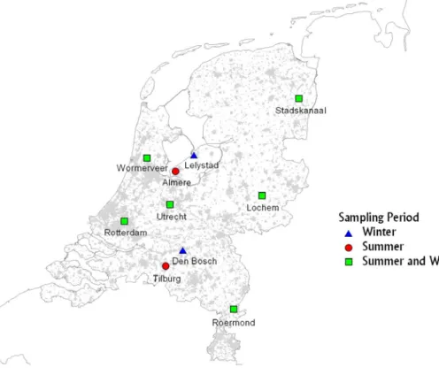
For each type of vegetable 8 volunteers bought sufficient material in shops at locations all over the Netherlands (Figure 1). The vegetables were divided into two categories, namely summer vegetables and winter vegetables. The summer vegetables were purchased in July 2001 and the winter vegetables in January 2002. The stores were selected to be representative for the stores where most of the vegetables are usually bought. The volunteers also registered the country of origin of the various vegetables. The large majority of the vegetables where harvested in the Netherlands. An exception was the French beans which were also imported from France, Spain, Egypt and Senegal. The volunteers were also asked to register whether or not vegetables were grown in greenhouses. Unfortunately this information often was not available in the stores.

Figure 1. Location of the stores where the vegetables were bought.

(9)

3 Analysis

3.1 Sample preparation

Visual soil and other dirt was removed from the vegetables. The non-edible parts were removed. From each sample 30 g was taken as representatively as possible. These parts were combined to make a pooled sample out of the eight individual samples. Unfortunately two individual spinach samples and one beet root sample were not available, therefore the pooled spinach and beet root samples were based on 6 and 7 individual samples, respectively. For each pooled sample also an analogon was made based on the same samples which were washed with cold water. These samples and the remainder of the individual samples were stored and available for further investigations.

Sample extraction and clean up

To the test portions, a solution of toluene containing 13C12-labeled internal

quantitation standards (Cambridge Isotope Laboratories, Woburn, MA, USA) of the 2,3,7,8-chlorine substituted PCDDs and PCDFs, and non-ortho PCBs 77, 81, 126 and

169 was added at levels between 0.6 and 3.2 pg/g vegetable. 13C12-labeled OCDF was

excluded to avoid interference with OCDD analysis. After freeze drying and refluxing with dichloromethane extracts were brought onto the top of a Carbosphere column.

Then an Al2O3 clean up took place. All eluates were evaporated to dryness and

redissolved in 50 µl of toluene containing an internal sensitivity standard (PCDD/F

analysis: 13_C

6-labeled 1,2,3,4-TeCDD; PCB analysis: 13C12-labeled PCB 80) at a

concentration of 2.4-2.5 ng/ml of toluene.

Gas chromatography - mass spectrometry

GC/MS analyses were performed on a VG70SQ or AutoSpec (Micromass, Manchester, UK) mass spectrometer coupled to a HP 5890 (Hewlett Packard, Palo Alto, MA, USA) gas chromatograph. GC separations were carried out on a non-polar column (60 m DB-5MS ; J&W Scientific, Folsom, USA; 0.25 mm ID, 0.10 µm film thickness). The temperature programme for PCDD/F analysis consisted of an isothermal period (150°C, 1 min), a rise at 10°C/min to 200°C, then at 2.5°C/min to 290°C and finally a second isothermal period of 4 min at 290°C. The temperature programme for non-ortho PCB analysis consisted of an isothermal period (90°C, 1 min), a rise at 10°C/min to 290°C, and finally a second isothermal period of 10 min at 290°C.

In all cases, helium was used as carrier gas at a linear velocity of 30 cm/s. Samples for PCDD/F analysis were injected by use of a solid all glass falling needle injector (Fa. Koppen, Best, The Netherlands). Samples for the non-ortho PCB analysis were injected using a CTC-A200s (CTC-Analytics, Zwinger, CH) autosampler on a split/splitless injector.

The GC/MS interface was maintained at 290°C in all cases. Ionization of samples was performed in the electron impact mode (EI) with 31 eV electrons. Instruments were operated at increased resolution. The resolving power (RP) was typically 5000 (VG70SQ) or 3000 (Autospec). Detection was performed by selected ion recording.

(10)

Limit of detection (LOD) and blanks

For each sample/congener combination the Limit Of Detection is (LOD) determined as a signal to noise ratio of 3. To control blank levels also procedural blanks and blank samples (peeled cucumber) were analysed. For some congeners low levels of dioxins in these blank samples could be detected. Results were not corrected for these levels in the blanks. The levels of TEQ have been calculated assuming non-detects equal to zero (lower bound estimates) and non-detects equal to LOD (upper bound estimates).

Estimate using pattern information (multiple imputation)

When a data set contains a number of results below the LOD several algorithms can be used to estimate the most likely value for the TEQ. In a recent publication several strategies were tested on a nearly complete, but artificially censored data set of dioxins in cow’s milk (Hoogerbrugge and Liem, 2000). In that study the multiple imputation algorithm appeared to have the smallest error of prediction and an adequate estimate for the uncertainty.

In the multiple imputation algorithm (Geman and Geman, 1984) any value below the detection limit in principle is replaced by a model value. However, instead of the model value itself a random value from a normal distribution around the model value is drawn. The standard deviation of this distribution is equal to the residual standard deviation between the model and the measured values.

In the resulting iteration process the levels of the first congener of all the samples of the dataset in which this congener is a non-detect are modelled using the concentrations of other congeners. The ‘old’ starting values on the positions of the non-detects are replaced by new imputations. Then the concentrations of the second congener are modelled and imputed and so on. After imputation of the last congener the iteration is continued with re-imputating the first congener etc. until 1000 iterations have been performed. In the iteration process some imputation candidates might be larger than the limit of detection. These candidates are rejected and a new candidate from the normal distribution is generated etc.

In the implementation of the multiple imputation as applied in this study the following choices were made:

- the model for each congener is generated using a regression model of the first 2 principal components (Principal Component Regression, PCR), (Massart, 1997). For the calculation of the principal components all other congeners are used. Principal components are used to reduce the number of independent variables with a minimum loss of information.

To obtain a full reflection of uncertainty rather extreme starting values were chosen: 1) Normal distributed random data with mean and standard deviation of the detected values; 2) Equal to the detection limit (LOD); 3) Equal to 0.01*LOD 4) Equal to 0.1*LOD.

The entire calculation is carried out for two data sets. In the first data set the data are logtransformed, which is in line with the assumption that the measurement uncertainty is proportional with the measured concentration. The second data set consisted of the original data, in line with the assumption that the measurement uncertainty is concentration independent. For the intake calculation (and for Figure 2) only the transformed data are used. The estimated uncertainty is based on both data sets.

(11)

3.2 Average intake of dioxins due to vegetable

consumption

In calculating the human exposure to dioxins the concentrations in consumed products are combined with the consumption rate of the products.

The consumption of the Dutch population was examined with the Dutch National Food Consumption Survey (DNFCS, Kistemaker et al., 1998). This survey describes the consumption of the Dutch population and includes information on the daily consumption over two consecutive days and a record of age, sex and body weight of 6250 individuals (Kistemaker et al., 1998). Usage of the DNFCS in calculating dietary intakes requires the concentration to be known in much more detail, i.e. at the level of the individual products of the Dutch Nutrient Databank (‘NEVO-products’; NEVO, 1996). Assignment of the NEVO-codes to the vegetables analysed contained two steps, namely 1) the summation of all products from the same vegetable (for example fresh, frozen and chopped) and 2) the combination of vegetables with similar characteristics.

(12)

4 Results and Discussion

4.1 Concentrations in vegetables

4.1.1 Analytical chemical results

The results of the analytical chemical analysis are summarised for each vegetable and for each congener in Appendix 1. In the analyses of the summer vegetables extremely low detection limits were obtained (< 1 pg/kg wet weight for each congener). Due to this low detection limit it is obvious that all summer vegetables have a toxic equivalent (TEQ) that is lower than 10 pg TEQ/kg fresh weight (FW). The results show that differences between the various vegetables exist which generally follow the assumption that vegetables with a high surface to volume ratio (such as endive and spinach) have relatively high concentrations and that vegetables with a low surface to volume ratio (such as tomato and cucumber) have relatively low concentrations. Another observation from the data is that in general for all components in each vegetable a strong consistency between the congener pattern seems to be present. The analyses of the winter vegetables were less successful with regards to a higher limit of detection. Therefore the differences between the upper and lower bound results are relatively large. This higher detection limit is presumably partly due to the difference in consistency between summer and winter vegetables since the latter are known to contain higher contents of interfering components like a waxy surface layer. On the other hand, the results for the blank and the cucumber are different for winter and summer, which indicates that for the winter vegetables the method or the instrument did not perform according to the standards as shown for the summer vegetables (Appendix 2). This difference was mainly caused by a much higher background which could not be solved by the various additional clean up steps that have been performed.

From the results one observation is very clear: curly kale shows much higher levels than any other vegetable analysed. This has been predicted and observed before since curly kale is famous for its large surface/content ratio, for a thick wax layer that perfectly absorbs hydrophobic contaminants, and for it’s extremely long presence on the field (9 months).

(13)

4.1.2 Multiple imputation

There is a large difference between the lower and upper bound estimates of the winter vegetables (Appendix 1). Below, a more accurate estimate for the most likely dioxin TEQ in the vegetable samples will be calculated. An important observation before starting this calculation is the fact that the patterns of the summer vegetables and of the curly kale show large similarities. This indicates that this similarity likely exists throughout our whole data set and can be used for a more precise estimate of the TEQ. For this reason all data are compiled into one data set and used as input for our multiple imputation algorithm.

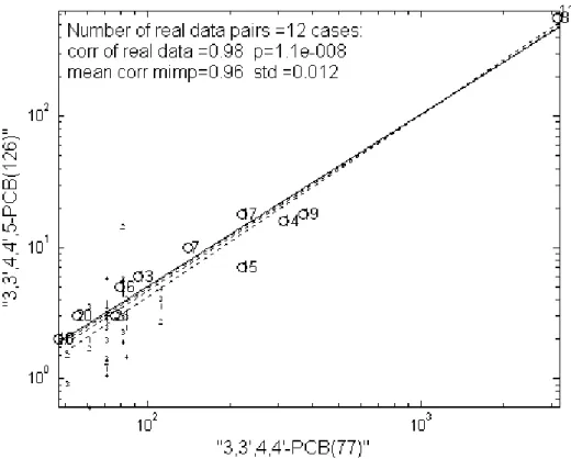
Figure 2 illustrates on a logarithmic scale the correlation between PCB-126 with PCB-77. The compound PCB-126 was detected in 12 from the 21 samples, while PCB-77 was present in all samples. The plot also shows the values that are generated by the multiple imputation algorithm as small numbers. For each of the four data sets (originating from the four different starting values) the regression is shown as dashed lines. According to the model the scatter of the imputed values should be part of the same distribution as the scatter of the detected values. The plot indicates that this objective is reasonably well achieved.

Figure 2. Correlation between concentrations of PCB-126 (pg/kg FW) and PCB-77 (pg/kg FW) in vegetables. The continuous line shows the relation based on the levels that were detected. The large numbers show the particular sample as used in Appendix 1 and 2 (11 and 8 are the curly kale samples). The small numbers show the imputed values for the four data sets. The relations based on both detected and imputed data are shown as dashed lines .

Using the imputed concentrations the TEQ values can be estimated. The results, indicate that the most likely multiple imputation estimate, especially for the winter vegetables, is much closer to the lower bound estimate than to the upper bound

(14)

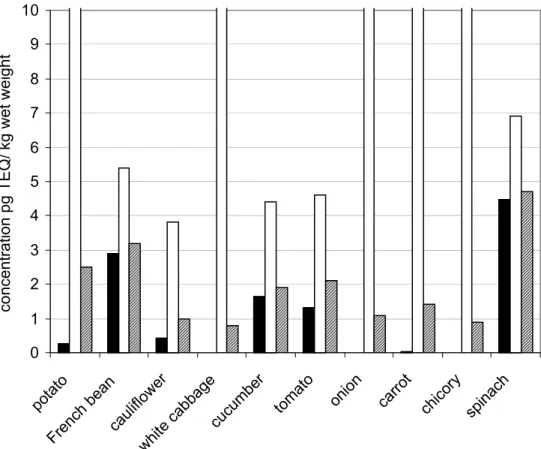
estimate (for the ten most important vegetables, see Figure 3). The explanation is probably that for most winter vegetables the observed levels of PCB 77 are low compared to the level in curly kale (<< 10 %) and to the leafy summer vegetables (<30 %) and also that some of the detection limits observed are lower than these levels. 0 1 2 3 4 5 6 7 8 9 10 potato Fren ch be an cauli flowe r white cabba ge cucu mbe r tom ato onion carro t chico ry spin ach concent ra tion pg T E Q/ kg w e t w e ight

Figure 3. Lower bound (black bars), upper bound (white bars) and most likely (hatched bars) concentrations of the sum of dioxins, furans and dioxin-like PCBs (pg TEQ/kg wet weight) in the ten vegetables with the highest consumption in the Netherlands. For five vegetables, the value of the upper bound levels are out of scale.

4.2 Average intake due to the consumption of vegetables

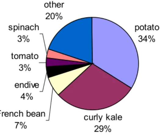
The average intake of dioxins by the DNFCS participants was estimated by multiplication and summation of the average consumption of the various vegetables per capita with the concentrations in these vegetables (Appendix 1). It appears that the total intake varies from 0.008 (lower bound) to 0.127 (upper bound) pg TEQ/kg bw/day, whereas the most likely intake is 0.014 pg TEQ/kg bw/day. The calculated uncertainty is 0.003 pg TEQ/kg bw /day. The highest contributions to the total intake by vegetables originates from potatoes and curly kale (Figure 4), the former because of the high consumption of potatoes and the latter because of the high concentrations in curly kale. Note that the uncertainty in the contribution of potatoes is relatively high (relative standard deviation of 68 %).

(15)

potato 34% curly kale 29% French bean 7% endive 4% tomato 3% spinach 3% other 20%

Figure 4. Contribution of the individual vegetables to the total dioxine intake. Under the category French bean also butter-bean, broad bean, garden pea and mange-tout are included, while the category tomato comprises tomato, but also pepper and courgette.

Comparison with levels found in composite samples.

In the intake study of Freijer et al. (2001) the levels found in the composite samples were 60 (lower bound) to 66 (upper) pg per kg vegetable. As indicated, this number was very uncertain due to several analytical problems. The average level in the vegetables without potatoes and curly kale calculated in this study is only 1.5 (lower bound) to 25 (upper bound) pg/kg vegetable. These data are not directly comparable since the composite sample for example contained spinach with cream and this cream was not present in the samples in this study. Despite these differences the conclusion still can be drawn that levels in this study are much lower than the levels estimated by Freijer et al. This difference might be due to contamination problems as described by Freijer et al.

For the contribution to the total intake this implies that the contribution was overestimated in the study of Freijer et al. and that the contribution of the consumption of vegetables to the total dietary dioxin intake is in the range 1-10 % and most likely at the lower end of this range.

Comparison with levels found in other countries

Recent data of dioxins (PCDDs/PCDFs only) in vegetables are available from Japan and Korea (Kwon et al., 2002). Spinach from Japan and Korea shows levels from 100-170 pg TEQ /kg spinach, which is much higher than the level found in this study. Levels found in other vegetables are much lower. Unfortunately in the lower bound presentation of the data the presumably large influence of the non-detects is not quantitatively indicated.

A study on British vegetables (Lovett et al., 1997) showed upperbound levels varying between 100-900 pg i-TEQ/kg for several vegetables and fruit. The low range of this data are determined by the values set at the detection limit. On the other hand in general these data seem to be considerably higher than the values reported in our study.

(16)

In an American vegetable composite sample all toxic PCDDs/PCDFs are below their limit of detection of 10-60 pg/g (Scheckter et al., 1997). The information content in this observation obviously is not very large. The only conclusion that can be drawn is that analysis of a mixture of our samples presumably would have given the same result.

Comparison with previous data

Dutch curly kale samples were analysed in 1991. In this study the level in background locations was around 1000 pg TEQ/ kg FW. This indicates that levels in kale are decreased considerably which coincides with the decrease in the emission of the major sources affecting the Dutch air.

(17)

5 Conclusions

Vegetables are analysed for toxic PCDDs/PCDFs and no-PCBs. Summer vegetables could be measured very sensitively. Upper bound levels vary between 3 and 10 pg TEQ/kg FW. Winter vegetables were measured less sensitively (LOD approximately 10 pg/kg per congener). Upper bound levels (with exception of curly kale) vary between 30 and 70 pg TEQ/ kg FW. The average level in curly kale is estimated as 100-200 pg TEQ/ kg FW.

Using upper bound levels the average intake of PCDDs/PCDFs and no-PCBs is estimated as 0.12 pg TEQ/kg bw/day. When a consistency of patterns between detected and non-detected levels is assumed, the most likely estimate is 0.014 pg TEQ/kg bw /day. The latter is less than 2 % of the mean total daily intake.

(18)

References

Baars, A.J., Theelen R.M.C., Janssen P.J.C.M., Hesse J.M., Apeldoorn M.E. van, Meijerink M.C.M., Verdam L., and Zeilmaker M.J. (2001) Re-evaluation of human-toxicological maximum permissible risk levels . Report number 711701025, National Institute for Public Health and the Environment, Bilthoven, The Netherlands.

Baars, A.J.,Bakker, M.I., Baumann, R.A., Boon, P.E., Freijer, J.I., Hoogenboom,

L.A.P., Hoogerbrugge, R., Van Klaveren, J.D., Liem, A.K.D., Traag, W.A. and De Vries, J. (2004) Dioxins, dioxin-like PCBs and non-dioxin-like PCBs in foodstuffs: occurrence and dietary intake in The Netherlands. Toxicology Letters 15: 51-61. EC (2001) European Commission, Council regulation No 2375/2001, Brussels,

Belgium.

Francken, J.M. (1999) Warenwetregeling verontreinigingen in levensmiddelen. Warenwet, Ministerie van Volksgezondheid, Welzijn en Sport, Directie Voeding en Veiligheid van Producten. Band 2, Levensmiddelen (A-12.1), p.3, Koninklijke Vermande BV, Lelystad, the Netherlands.

Freijer, J.I., Hoogerbrugge, R., Van Klaveren, J.D., Traag, W.A., Hoogenboom, L.A.P., and Liem, A.K.D. (2001). Dioxins and dioxin-like PCBs in foodstuffs:

Occurence and dietary intake in The Netherlands at the end of the 20th century.

Report number 639102022, National Institute for Public Health and the Environment, Bilthoven, the Netherlands.

Geman, S., and D. Geman. 1984. Stochastic Relaxation, Gibbs Distributions, and the Bayesian Restoration of Images. IEEE Transactions on Pattern Analysis and Machine Intelligence 6721-41.

Hoogerbrugge R. and A.K.D. Liem, How to handle non-detects, Organohalogen Compounds 45 (2000) 13-16.

Kistemaker, C., Bouman, M., and Hulshof, K.F.A.M. (1998) Consumption of separate products by Dutch population groups - Dutch National Food Consumption Survey 1997 – 1998 (in Dutch). TNO-report V98.812, TNO-Nutrition and Food Research Institute, Zeist, the Netherlands.

Kwon, O.-K., Eun, H-S, Uegi, M., Hong, S-M., Song, B-H., Lee, H-D., Park, C-H., and Ryu G-H. (2002) Organohalogen Compounds 57 113-116.

Liem, A.K.D., Theelen, R.M.C., Slob, W., and Van Wijnen, J.H. (1991). Dioxinen en planaire PCB’s in voeding. Gehalten in voedingsprodukten en inname door de Nederlandse bevolking. Report number 730501034, RIVM, Bilthoven, the Netherlands (In Dutch).

Liem, A.K.D., and Theelen, R.M.C. (1997). Dioxins. Chemical analysis, exposure and risk assessment. (Thesis), Research Institute of Toxicology (RITOX), University of Utrecht, The Netherlands; ISBN 90-393-2012-8.

(19)

Liem, A.K.D., Theelen, R.M.C., Hoogerbrugge R., and Jong A.P.J.M. de, (1993). Gehalte van dioxinen in boerenkool. Report number 730501048, RIVM, Bilthoven, the Netherlands (In Dutch).

Lovett, A.A., Foxall, C.D., Creaser C.S., and Chewe, D. (1997) Chemosphere 34, 1421-1436.

Massart D.L., Vandeginste, B.G.M., Buydens, L.M.C., de Jong, S., Lewi, P.J., and Smeyers-Verbeke, J. Handbook of Chemometrics and Qualimetrics, Elsevier, Amsterdam (1997).

NEVO (1996). NEVO-tabel Nederlandse Voedingsstoffenbestand 1996. Stichting NEVO, Voedingscentrum, Den Haag (In Dutch).

SCF (2001). Opinion of the SCF on the risk assessment of dioxins and dioxin-like PCBs in food. Update based on new scientific information avialable since the adoption of the SCF opinion of 22nd November 2000. European Commission, Scientific Committee on Food, Brussels, Belgium.

Scheckter, A., Cramer, P., Boggess, K., Stanley, J., and Olson, J.R., (1997) Chemosphere 34, 1437-1447.

SCOOP (2000) Assessment of dietary intake of dioxins and related PCBs by the population of EU member states. Final report 7 June 2000, Brussels, Belgium. Slob, W. (1993) Modeling long-term exposure of the whole population to chemicals

in food. Risk Analysis, 13:525-530

Voedingscentrum (1998) Zo eet Nederland 1998 (in Dutch). Voedingscentrum, Den Haag, The Netherlands; ISBN 90-5177-036-7.

(20)

Appendix 1: Concentrations of PCDDs, PCDFs and PCBs in Dutch consumer vegetables with several TEQ estimates and intake estimates

Vegetable

pot

ato oni_on carrot

chi cor y leek Bru ssel s spr out s cur ly kal e whi te cab bag e bee tro ot cuc um ber Fre nch bea n to mat o lett uce end ive lett uce Ice ber g spi nac h mu shr oo ms cau lifl ow er Inta ke [pg TE Q/ kg bw/ day ]

intake vegetable g/ kg bw/day 1.91 0.15 0.14 0.11 0.07 0.07 0.04 0.14 0.05 0.13 0.31 0.2 0.05 0.07 0.05 0.09 0.04 0.2

TEQ lower bound (pg/kg) 0.26 0.01 0.02 0.01 0.02 1.16 98.0 0.01 0.01 1.64 2.91 1.32 2.20 6.72 1.85 4.47 1.32 0.42 0.008

TEQ upper bound (pg/kg) 36.0 73.4 53.4 55.9 61.9 62.9 122.1 51.5 36.2 4.4 5.4 4.6 4.6 9.3 4.2 6.9 4.1 3.8 0.127

most likely TEQ (pg/kg) 2.5 1.1 1.4 0.9 1.7 2.6 100.2 0.8 1.5 1.9 3.2 2.1 2.5 7.1 2.3 4.7 1.7 1.0 0.014

uncertainty most likely TEQ (pg/kg) 1.7 1.4 0.8 1.3 0.6 0.8 5.1 0.5 1.3 0.1 0.5 0.7 0.4 0.7 0.4 0.7 0.4 0.9 0.003

Winter Summer dioxins (pg/kg) 2,3,7,8-TCDD <10 <30 <10 <20 <10 <20 <10 <10 <10 <1 <1 <1 <1 <1 <1 <1 <1 <1 1,2,3,7,8-PeCDD <10 <20 <20 <20 <20 <20 <10 <20 <10 <1 <1 <1 <1 <1 <1 <1 <1 <1 1,2,3,4,7,8-HxCDD <10 <10 <10 <10 <10 <20 21 <10 <10 <1 <1 <1 <1 2 <1 <1 <1 <1 1,2,3,6,7,8-HxCDD <10 <10 <10 <10 <10 <20 34 <10 <10 <1 <1 <1 2 4 1 2 3 <1 1,2,3,7,8,9-HxCDD <10 <10 <10 <10 <10 <20 46 <10 <10 <1 <1 <1 <1 3 1 <1 <1 <1 1,2,3,4,6,7,8-HpCDD <10 <10 <10 <10 <10 14 <50 <20 <40 13 14 20 27 51 23 33 17 6 OCDD 51 64 75 51 88 85 1536 54 59 85 114 146 240 305 162 247 73 67 furans (pg/kg) 2,3,7,8-TCDF <10 <30 <30 <10 <20 <20 27 <10 <10 <1 <1 <1 <1 <1 <1 <1 <1 <1 1,2,3,7,8-PeCDF <10 <20 <20 <10 <30 <10 <10 <20 <10 <1 1 <1 1 2 1 2 <1 <1 2,3,4,7,8-PeCDF <10 <20 <20 <10 <30 <10 46 <20 <10 1 1 <1 1 4 1 2 1 <1 1,2,3,4,7,8-HxCDF <10 <10 <10 <10 <20 <20 <10 <10 <10 <1 1 <1 1 <4 1 2 <1 <1 1,2,3,6,7,8-HxCDF <10 <10 <10 <10 <20 <20 <10 <10 <10 <1 1 <1 1 4 1 2 <1 <1 1,2,3,7,8,9-HxCDF <10 <10 <10 <10 <20 <20 <10 <10 <10 <1 <1 <1 <1 <1 <1 <1 <1 <1 2,3,4,6,7,8-HxCDF <10 <10 <10 <10 <20 <20 37 <10 <10 3 3 3 3 6 3 3 <1 <1 1,2,3,4,6,7,8-HpCDF 24 <10 <10 <10 <10 <10 140 <10 <10 8 6 8 14 30 13 22 4 4 1,2,3,4,7,8,9-HpCDF <10 <10 <10 <10 <10 <10 <10 <10 <10 1 1 <1 1 2 2 2 <1 <1 OCDF 63 <10 12 <10 13 12 109 <10 <100 9 10 13 20 39 18 37 5 <1 PCB's (pg/kg) 3,3',4,4'-PCB(77) 70 70 70 60 80 140 3130 50 80 92 315 221 79 222 47 372 55 76 3,4,4',5-PCB(81) <20 <20 <20 <20 <20 <20 240 <20 <20 15 21 23 8 9 8 25 11 9 3,3',4,4',5-PCB(126) <20 <20 <20 <20 <20 10 560 <20 <20 6 16 7 5 18 2 18 3 3 3,3',4,4',5,5'-PCB(169) <5 <5 <5 <5 <5 <5 60 <5 <5 <0.8 <0.8 <0.8 <0.8 3 <0.8 3 <0.8 <0.8 number in figure 2 2 3 4 5 6 7 8 9 10 13 14 15 16 17 18 19 20 21

Appe

n

dix 1

Concentations of PCDDs,

PCDFs and

PCBs

in

Du

tch

con

su

m

er veg

etab

les

with

s

ev

eral

TEQ estimat

es and intake estimat

(21)

Appendix 2 Concentrations of PCDDs, PCDFs and

control samples with several TEQ estimates (pg/kg)

Vegetable peel ed cucum ber (w inte r) digested curly kale peel ed cucum ber (sum m er)

TEQ lower bound 0.3 172.7 0.6

TEQ upper bound 85.9 384.7 3.5

most likely TEQ 2.5 190.1 1.3

uncertainty most likely TEQ (pg/kg) 1.2 8.5 0.6

dioxins 2,3,7,8- <60 <50 <1 1,2,3,7,8- <10 <20 <1 1,2,3,4,7,8- <10 <800 <1 1,2,3,6,7,8- <10 <400 <1 1,2,3,7,8,9- <10 <200 <1 1,2,3,4,6,7,8- 13 434 9 OCDD 90 1765 48 furans 2,3,7,8- <10 109 <1 1,2,3,7,8- <10 86 <1 2,3,4,7,8- <10 105 1 1,2,3,4,7,8- <10 163 <1 1,2,3,6,7,8- <10 89 <1 1,2,3,7,8,9- <10 <20 <1 2,3,4,6,7,8- <10 81 <1 1,2,3,4,6,7,8- 11 260 4 1,2,3,4,7,8,9- <10 45 <1 OCDF 42 460 4 PCBs 3,3',4,4'- 110 3190 82 3,4,4',5- <20 230 12 3,3',4,4',5- <20 630 <0.1 3,3',4,4',5,5'- <5 70 <0.8 number in figure 2 1 11 12

(22)

Appendix 3 Mailing list

1 Directeur-generaal, VWA

2 Directeur Onderzoek en Risicobeoordeling, VWA

3-5 Hoofdinspectie Levensmiddelen Keuringsdienst van Waren, VWA

6-8 Veterinair Hoofdinspecteur Keuringsdienst van Waren, VWA

9 Directeur Voeding en Gezondheidsbescherming, VWS

10 Directeur Voedings-, en Veterinaire Aangelegenheden, LNV

11 Hoofdinspecteur Milieuhygiëne, VROM

12 Directeur Stoffen, Afvalstoffen, Straling, VROM

13 Drs. G.A. Lam, KvW, VWA

14 Voorzitter Gezondheidsraad

15 Dr. R. Malisch, Chemisches und Veterinäruntersuchungsamt, Germany

16 Dr. S. Atuma, Swedish National Food Administration, Sweden

17 Dr. P.O. Darnerud, Swedish National Food Administration, Sweden

18 Dr. M. Rose, CSL, UK

19 Dr. A. di Domenico, Istituto Superiore di Sanita, Italy

20 Dr. A.K.D. Liem, EFSA, Brussels, Belgium

21 Mr. F. Verstraete, European Commission, Belgium

22 Dr. M.A. Slayne, European Commission, Belgium

23 Dr. Ch. Vinkx, Algemene Eetwareninspectie, Belgium

24 Dr. G. de Poorter, Federal Ministry of Agriculture, Belgium

25 Dr. R. van Cleuvenbergen, VITO, Belgium

26 Prof. Dr. L. Goeyens, Wetenschappelijk Instituut Volksgezondheid, Belgium

27 Dr. G. Becher, NIPH, Norway

28-37 Werkgroep Dioxinen in Voeding

38 Redactie Ware(n) ChemicusRedactie Voeding Nu

39 Ir. G. Kramer, Consumentenbond

40 Depot Nederlandse Publicaties en Nederlandse Bibliografie

41 Directie RIVM 42 Dr. ir. R.D. Woittiez 43 Ir. H.J.W.J. v.d. Wiel 44 Dr. L. A. van Ginkel 45 Dr. P. van Zoonen 46 Dr. E.A. Hogendoorn

47 Prof. dr. ir. D. van de Meent

48 Dr. M.G. Mennen

49 Dr. ir. M.N. Pieters

50 Dr. ir. A.J.A.M Sips

51 SBC/afd. Communicatie

(23)

53 Bibliotheek 54 Archief LAC 55 Archief SIR 56-70 Auteurs 71-75 Bureau Rapportenbeheer 76-80 Reserve exemplaren