Can we use CDS spreads to identify the monetary policy stance of the ECB?

(1)

CAN WE USE CDS SPREADS TO IDENTIFY THE

MONETARY POLICY STANCE OF THE ECB?

Aantal woorden/ Word count: 9.017

Loewy Lampaert

Stamnummer/ student number : 01709961

Promotor/ Supervisor: Prof. dr. Rudi Vander Vennet

Co-promotor/ Co-supervisor: Nicolas Soenen

Masterproef voorgedragen tot het bekomen van de graad van :

Master’s Dissertation submitted to obtain the degree of:

Master of Science in Economics

(2)

Deze pagina is niet beschikbaar omdat ze persoonsgegevens bevat.

Universiteitsbibliotheek Gent, 2021.

This page is not available because it contains personal information.

Ghent University, Library, 2021.

(3)

Foreword

This thesis wraps up my journey at Ghent University, where I have had the pleasure of following many insightful and challenging courses during the linking and master programme. I want to thank prof. Vander Vennet, who always enthusiastically shared his knowledge and whose courses encouraged me to pursue a career in the financial sector. I also want to express my gratitude to Nicolas Soenen, who helped me gain valuable insight into the topic and regularly made the time to follow up and answer questions. Furthermore, I’d like to acknowledge the effort of my proofreader Alexander and the continuous support of Laura, my friends, my parents and of course Bailey.

Loewy Lampaert June 1, 2020 Brussels

(4)

List of abbreviations

APP Asset purchase programme CAP Capital ratio

CCPs Central counter parties CDS Credit default swap CET Central European time DIV Diversification

DTL Deposits to liabilities ECB European Central Bank FED Federal Reserve

LLP Loan loss provisions

LTA Net loans to earnings assets LTRO Long-term refinancing operations MRO Main refinancing operations NIM Net interest margin

OMT Outright monetary transactions QE Quantitative easing

ROA Return on assets

SMP Securities market programme

(7)

List of Tables

2.1 Most important ECB policy announcement events (2008-2017) . . . 10

3.1 Factors proportion of total variance . . . 17

3.2 Estimated one-factor model . . . 20

4.1 Variable description and expected sign . . . 26

4.2 Baseline estimation results . . . 27

4.3 Subsample estimation results . . . 29

A.1 Sample European banks 2008-2017 . . . XII A.2 Summary statistics sample CDS premia (2008-2017) . . . XIII A.3 Summary statistics daily CDS returns (2008-2017) . . . XIV A.4 Eigenvalues to determine the number of factors . . . XV A.5 Estimated one-factor model . . . XVI A.6 Estimated monetary policy factor scores . . . XVII A.7 Correlation matrix of explanatory variables . . . XVIII A.8 Summary statistics quarterly and yearly panel models . . . XVIII A.9 Hausman test of the baseline models . . . XVIII A.10 Hausman tests of the subsample models . . . XIX

(8)

List of Figures

1.1 Evolution of the main refinancing operations rate, own creation based on ECB

data. . . 1

1.2 Evolution of the notional amounts outstanding of total CDS contracts (2004-2019), own creation based on BIS data. . . 5

1.3 Outstanding notional amounts of CDS contracts per type of institution in 2019, own creation based on BIS data. . . 6

2.1 Evolution of the average daily 5y CDS spread of 40 European banks (2008-2016), own creation based on Bankscope data. . . 9

3.1 Scree graph of the eigenvalues . . . 18

4.1 Factor scores over time . . . 23

(9)

1 Introduction

1.1 Setting the scene

Following the global financial crisis of 2007-2009 and the European debt crisis of 2010-2012, the monetary policy conducted by the ECB has mainly been very accommodative while deploying a whole toolbox of conventional and non-conventional measures. The interest rate on the main refinancing operations (MRO) has been gradually lowered to 0% (figure 1.1), while the inter-est rate on the deposit facility was lowered to an all-time low of -0,50% 1. Next to negative

0.00 0.25 0.50 0.75 1.00 1.25 1.50 1.75 2.00 2.25 2.50 2.75 3.00 3.25 3.50 3.75 4.00 4.25 2007 2008 2009 2010 2011 2012 2013 2014 2015 2016 2017 2018 2019 2020 % 11/01/2007−12/03/2020

Main refinancing operations rate (MRO)

Figure 1.1: Evolution of the main refinancing operations rate, own creation based on ECB data.

deposit rates, other unconventional tools that were utilized were different waves of long-term refinancing operations (LTRO) and targeted long-term refinancing operations (TLTRO) with varying maturities, which aim to provide liquidity to commercial banks. The securities market programme (SMP) was launched in 2010 amidst the Greek government debt crisis and consisted

(10)

Introduction

of purchasing government bonds on the secondary market. Further on in 2012 at the peak of the Euro crisis, Outright Monetary Transactions (OMT) was announced following the ‘whatever it takes’ mantra of former president of the ECB Mario Draghi. Although these measures narrowed spreads on the financial markets, the unlimited purchases of government securities on the sec-ondary market was never activated. Next, the first wave of the asset purchase programme (APP) or quantitative easing (QE) was initiated in the beginning of 2015 and lasted until the end of 2018. It involved the ECB purchasing mainly government bonds for an amount of 60-80bn EUR per month. The programme was reactivated in November 2019 at an initial pace of 20bn EUR net bond purchases per month, but was expanded along with other expansionary measures in reaction to the coronavirus outbreak2_{. At last, an important tool of communication is forward}

guidance which provides clear information about the future path of interest rates. The ultimate aim of these policies is to raise inflation expectations and achieve the ECB’s inflation target of close to, but below, 2%.

In this thesis, we are going to incorporate the monetary policy announcements of the ECB from 2008 until 2017. Based on bank CDS spreads, we aim to identify the monetary policy stance. Furthermore, we also want to examine which bank business models react more or less sensitive to these policy measures.

1.2 Monetary policy and asset returns

An extensive literature is available which examined the financial market’s response to monetary policy announcements. Regarding anticipated monetary policy measures, they are found to have little effect on asset prices, while unanticipated changes carry a large and significant impact (Kuttner, 2001; G¨urkaynak et al., 2005; Swanson, 2017). Bernanke and Kuttner (2005) found that on average, an unanticipated federal funds rate cut of 25bp is associated with a one percent inrease in broad stock indexes. In general, it is found that unanticipated expansionary measures have a positive impact on stock markets, while unanticipated restrictive measures and policy inaction have a negative impact. Madura and Schnusenberg (2000); Kuttner (2001); Bernanke and Kuttner (2005); Rigobon and Sack (2004) confirm this for monetary policy actions conducted by the FED. The same holds for policy actions conducted by the ECB (e.g. Bohl et al., 2008; Fiordelisi et al., 2014; Boeckx et al., 2017; Altavilla et al., 2019). Although it has to be mentioned that monetary policy surprises only explain a fraction of the stock prices’ overall variability (Bernanke and Kuttner, 2005).

2

ECB announces 750 billion EUR Pandemic Emergency Purchase Programme (ECB Press release, 18 March 2020). Source: www.ecb.europa.eu

(11)

Introduction

More recently, the focus has mainly been on the impact of unconventional measures such as QE and forward guidance following the global financial crisis and due to central banks such as the FED3 and ECB reaching the zero lower bound. Regarding the US, Swanson (2017) investigated the effects of forward guidance and large scale asset purchases during the zero lower bound period (2009-2015). They concluded that both unconventional measures had a significant impact on Treasury yields and stock prices similar to the effects of the federal funds rate before reaching the zero lower bound. Forward guidance had a greater effect on short-term Treasury yields, while quantitative easing was more effective at lowering long-term Treasury yields and corporate bond yields. Concerning the eurozone, Altavilla et al. (2019) found that monetary policy surprises that increase yields lead to a European stock market decline. Moreover, they concluded that forward guidance and QE surprises were both succesful at lowering longer-term yields. In addition, QE was found to have lowered all yields across maturities and successful at narrowing spreads.

Accomodative monetary policy measures were also found to have had a positive effect on bank stock returns and bank stability (e.g. Madura and Schnusenberg, 2000; Yin et al., 2010; Yin and Yang, 2013; Kim et al., 2013; Fiordelisi et al., 2014; Ricci, 2015; Altavilla et al., 2017; Lamers et al., 2019). Studies that investigated the heterogeneous response to policy announcements across bank business models are the closest related to this thesis. Some important findings are that banks with lower capital ratios are more exposed to monetary policy announcements (Madura and Schnusenberg, 2000; Yin and Yang, 2013; Ricci, 2015; Lamers et al., 2019). Banks with more non-deposit funding are also found to be more responsive to changes in monetary policy (Yin and Yang, 2013; Ricci, 2015). According to Lamers et al. (2019), banks with a higher asset risk experience a reduction in systemic risk following an expansionary monetary policy shock. Furthermore, banks reacted more sensitively to non-conventional measures than to interest rate announcements (Fiordelisi et al., 2014; Ricci, 2015). We expect to find similar results across bank business models when employing bank CDS spreads.

However, studies that deal with bank credit default swap spreads are rather limited. One group in the literature focussed on the determinants of bank CDS spreads (e.g. Annaert et al., 2013; Chiaramonte and Casu, 2013; Babihuga and Spaltro, 2014; Samaniego-Medina et al., 2016; Drago et al., 2017). Another group investigated bank fragility and contagion through bank- and sovereign CDS spreads (e.g. Eichengreen et al., 2012; De Bruyckere et al., 2013; Acharya et al., 2014; Ballester et al., 2016). In the next chapter we will focus on these areas more in depth.

3

The federal funds rate was lowered to 0-0,25% from 15-12-2008 until 14-12-2015. However in a swift response to the coronavirus outbreak, the FED cut its federal funds rate again to 0-0,25% as of 16-03-2020. Source: www.federalreserve.gov

(12)

Introduction

Nonetheless, the reaction to the monetary policy announcements of the ECB including the non-conventional measures and identifying the underlying bank business models of this reaction using bank CDS returns remains a rather unexplored topic. We do expect to find a negative effect of expansionary central bank balance sheet measures on bank CDSs, which would be in line with the estimates of Boeckx et al. (2017); Altavilla et al. (2017). In addition, the CDS market yields several advantages over bond and equity markets with regard to price discovery and liquidity, and contribute supplementary information next to what is contained by equity markets and accounting metrics (Avino et al., 2019). We will investigate these advantages in the following section.

1.3 Credit default swaps

1.3.1 Definition

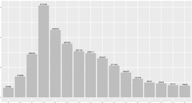
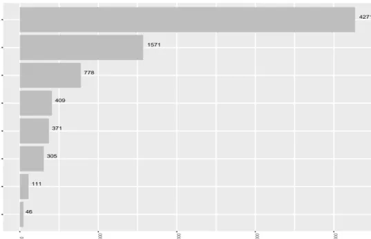
Introduced in the 1990’s by JPMorgan, a credit default swap (CDS) is a financial derivative or an insurance contract between two parties whereby the CDS seller agrees to compensate the CDS buyer for the losses incurred in case a certain credit event takes place such as bankruptcy, loan default or obligation default. The periodic premium paid by the CDS buyer to the CDS seller for transferring the risk of a credit event is called the CDS spread (Annaert et al., 2013). In essence CDS contracts allow the credit risk to be transferred and managed, but they also imply exposure to the default risk of the CDS seller. Because CDS contracts are traded over the counter (OTC), the market size has to be approximated. The Bank of International Settlements (BIS) uses the CDS exposures of about 70 banks and other brokers based in 12 other countries in their methodology. Leading up to the global financial crisis, the total outstanding notional amount of CDS contracts doubled each year from 2004 (6,4tn USD) until its peak in 2007 (61,2tn USD) but was reduced drastically to 9,4tn USD one decade later and has been on the decline ever since (figure 1.2). The main reason for this decline in the direct aftermath of the financial crisis is compression of CDS contracts (Aldasoro and Ehlers, 2018). Portfolio compression reduces the gross individual positions without affecting the net positions by terminating existing contracts and replacing these with new ones which have a lower total notional values. The more recent market developments are attributed to the rise in central counterparties (CCPs) and the decline in inter-dealer positions (Aldasoro and Ehlers, 2018). Pushed forward by financial regulators, CCPs intermediate and clear transactions between two parties where they takeover part of the credit risk (Heider et al., 2017). Nevertheless CDS contracts remain a very actively traded instrument and owned by a wide variety of institutions (figure 1.3).

(13)

Introduction 6396 13908 28650 61242 44943 35783 30718 29511 25937 21142 16507 12379 9931 ₉₃₅₄ 8141 7809 0 20000 40000 60000 2004 2005 2006 2007 2008 2009 2010 2011 2012 2013 2014 2015 2016 2017 2018 2019 Year

Total notional amounts outstanding

In billion USD

Total CDS contracts (2004 − 2019)

Figure 1.2: Evolution of the notional amounts outstanding of total CDS contracts (2004-2019), own creation based on BIS data.

1.3.2 Motivation

In comparison with bank accounting based measures, CDS spreads are forward looking. They incorporate all available information regarding the expected default risk, while the balance sheet information is only available ex-post. Bank CDS spreads especially capture the risk reflected by bank balance sheet ratios (Chiaramonte and Casu, 2010). Furthermore CDS spreads are immediately updated while accounting based measures are subject to the quarterly reporting period.

In addition, CDSs feature several advantages over bond yields as a market measure of risk. Speculative trading is mostly concentrated in the CDS market and less in the underlying bond market due to smaller trading frictions. Investors with short trading horizons tend to prefer the relative liquidity advantage of the CDS market over the underlying bond (Oehmke and Zawadowski, 2017). Longstaff et al. (2005) found evidence that the CDS market is more liquid than the corporate debt market. According to Blanco et al. (2005) and Norden and Weber (2009), the CDS market leads the bond market in price discovery but this deviation is mainly short-lived and is more pronounced in the US.

When comparing price discovery of CDS markets to equity market, the evidence is less clear-cut. Acharya and Johnson (2007) found empirical evidence for the existence of an information flow from the CDS market to the equity market. But this only occurs for negative credit events and for entities that previously occurred significant shocks. On the other hand, Narayan et al.

(14)

Introduction 1571 4271 409 111 46 371 778 305 SPVs, SPCc, SPEs Insurance and financial guaranty firms Non−financial institutions Hedge funds Banks and securities firms Other financial institutions Reporting dealers CCPs

0

1000 2000 3000 4000

Notional amounts outstanding In billion USD

Total CDS contracts per type of institution in 2019

Figure 1.3: Outstanding notional amounts of CDS contracts per type of institution in 2019, own creation based on BIS data.

(2014) argue that equity markets contribute more to price discovery than CDS markets in the majority of sectors, and in sectors where both equity markets and CDS markets contribute to price discovery, equity markets dominate this process. Nevertheless, bank specific CDS spreads supplement the information contained by equity markets and accounting metrics according to Avino et al. (2019). They find that an increase in bank CDS spreads is significantly associated with an increase in probability of future default of the bank.

1.4 Research questions and overview

The first main question that we aim to answer is if we can identify the monetary policy stance of the ECB based on bank CDS spreads. Secondly, we want to examine which bank business models are more exposed to monetary policy announcements, while including conventional and unconventional measures, based on the bank specific change in CDS spread on the respective policy announcement dates between 2008 and 2017. In the next chapter, we will deal with the literature about bank CDS spreads, give an overview of our data and describe our factor and econometric models. Chapter 3 will contain the methodology of our factor analysis and econometric model applied to our data. The regression output and interpretation of the results will be discussed in chapter 4. In our final section we will highlight the relevant results and wrap up with a conclusion.

(15)

2 Literature

2.1 Determinants of bank CDSs

We will start with the group of literature that focuses on the determinants of bank CDSs. It is important to make a distinction between corporate and bank CDSs when analyzing the determinants. The reasons are different financial structures, different relevant ratios 1 and loss of explanatory power when applying variables that affect credit spreads of corporations to banks (Drago et al., 2017). Annaert et al. (2013) analysed the CDS spread determinants of 32 euro area banks for the periods before and during the global financial crisis. The explained part of the CDS spread changes is decomposed in credit risk, liquidity and business cycle factors. They find that CDS spreads are not uniquely driven by credit risk factors but also by individual liquidity, market liquidity and business cycle factors. Furthermore these determinants are time-varying but less so across rating categories. During the global financial crisis, the sharp increase in CDS spreads was initiated by an increased credit risk, but individual and market liquidity were found to be the dominant factors of that period. Chiaramonte and Casu (2013) focused on accounting-based ratios when examining the determinants of bank CDS spreads. Their sample consisted of 57 international banks, including 43 European banks, and ranges from 2005 until 2011. During the global financial crisis, they found that the risk captured by accounting-based measures are well reflected by bank CDS spreads. In addition they also concluded that the determinants are time-varying depending on different economic and financial conditions. Babihuga and Spaltro (2014) used bank CDS spreads as a proxy for bank unsecured funding costs. According to their results, changes in bank CDS spreads are associated with credit worthiness and changes in the level and quality of the bank’s capital. Moreover, domestic economic conditions and short term interest rates are related, as well as global risk factors. Samaniego-Medina et al. (2016) incorporated CDS spreads of 45 European banks between 2004 and 2010. They incorporated accounting and market-based variables, individual liquidity, market liquidity and business cycle

1_{One indicator of financial strength for corporations is the current ratio. This is the ratio of current assets}

and current liabilities. These are not typically found on bank balance sheets because they do not include e.g. accounts payable and inventories. An alternative for banks would be to look at the net interest margin (NIM).

(16)

Literature

factors to investigate the determinants of bank CDS spreads. Their main finding is that market-based variables yield the most explanatory power and that the explanatory power of the model was higher during the global financial crisis than before. Finally, Drago et al. (2017) extend the literature by including a longer time horizon 2007-2016 and more cross-country variation (US, core and periphery eurozone countries) when analyzing the determinants of bank CDS spreads. Their findings indicate that wider bank CDS spreads are related with lower capital ratios, higher leverage, lower asset quality, less stable funding, lower credit rating of the bank and a more subdued business outlook. Furthermore, sovereign risk and bank size were also found to be important determinants.

2.2 CDSs and bank fragility

Bank and sovereign CDS spreads are also used in empirical studies which explore bank fragility and contagion. Eichengreen et al. (2012) utilized principal component analysis to identify com-mon factors in the change of 45 bank CDS spreads in Europe and the US from 2002 until 2008. Their results indicate that a common factor existed in the period before the global financial crisis and was mainly related to the macroeconomic environment. This common factor became significantly more important during the global financial crisis and its importance was initially driven by the deteriorating creditworthiness of the banking sector. After the collapse of Lehman Brothers, funding risk became a more important driver of the common factor while the worsened economic outlook contributed to the increase in spreads. De Bruyckere et al. (2013) found evi-dence of sovereign-bank contagion during the European financial and sovereign debt crisis, using CDS spreads as a measure of credit risk. They defined contagion as the excess correlation be-tween banks and sovereigns in addition to the explained part of the common factors, their results indicate that banks with lower capital ratios, less stable funding and less retail-oriented are more exposed to risk spillovers. Acharya et al. (2014) also examined the sovereign-bank contagion us-ing CDS spreads. They show that countries with a lower credit ratus-ing, higher levels of debt, and part of a monetary union have a stronger sovereign-bank CDS relationship. Finally, Ballester et al. (2016) incorporated a sample of 55 European and US bank CDS spreads. They used principal component analyses to distinguish between common and idiosyncratic components in CDS spread changes. Their results provide evidence for both common and idiosyncratic types of contagion. The systematic contagion was found to be always greater than the idiosyncratic counterpart with time-varying dynamics.

(17)

Literature

2.3 Data

2.3.1 Bank CDS spreads

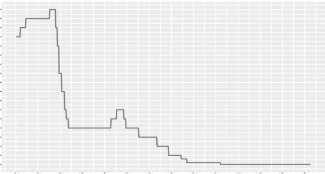
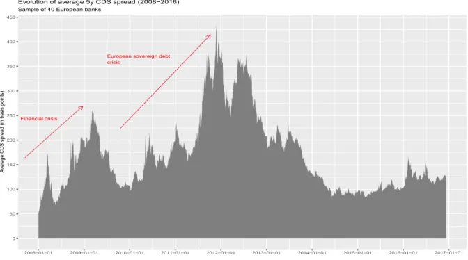
In this section, we will present the data used in this thesis obtained from the Bankscope database. For the full list of banks in this sample, we refer to table A.1 in the appendix. Our sample consists of daily CDS spreads with a 5-year maturity from 40 European banks in the period of October 2008 until December 2016. We make use of daily data in order to isolate the period of the ECB policy announcement and limit the impact of other macroeconomic events on the change in CDS spreads. The choice of 40 banks is not random, but based on completeness and availability of the data. Regarding the maturity, the market for 5-year CDS contracts is agreed to be the most liquid (V¨olz and Wedow, 2011; Annaert et al., 2013; Samaniego-Medina et al., 2016). The CDS spread is the percentage of the notional amount the CDS buyer needs to pay yearly to the CDS seller for the duration of the contract. A higher CDS spread indicates the market’s view of a higher default probability. Figure 2.1 shows the average evolution of our CDS spread sample. We can distinguish two significant moves on the graph. The first sharp increase in spreads was

0 50 100 150 200 250 300 350 400 450 2008−01−01 2009−01−01 2010−01−01 2011−01−01 2012−01−01 2013−01−01 2014−01−01 2015−01−01 2016−01−01 2017−01−01 Av er ag e C D S sp re ad (i n ba si s po in ts )

Sample of 40 European banks

Evolution of average 5y CDS spread (2008−2016)

Figure 2.1: Evolution of the average daily 5y CDS spread of 40 European banks (2008-2016), own creation based on Bankscope data.

during the global financial crisis, where the US subprime mortgage crisis and events such as the collapse of Lehman brothers contributed to the increase in credit risk. While the CDS spread of US banks rose to unprecedented levels, spreads of European banks increased to a lesser extend. (Babihuga and Spaltro, 2014). European bank spreads widened the most during the sovereign

(18)

Literature

debt crisis. The first sharp increase during this period is marked by Greece when the country requested a bailout from the European troika in April 2010. Spreads continued on to reach all time highs as sovereign-bank contagion fears peaked. Following Draghi’s ’whatever it takes’ speech in July 2012 and the announcement of OMT in September 2012, spreads have seen a steady decline but remain at elevated levels relative to the global financial crisis.

2.3.2 ECB policy announcements

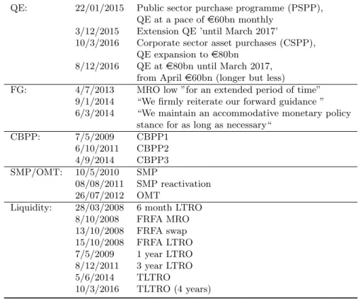
Next we have the policy announcement dates of the ECB which will be used to calculate the change in bank CDS spread on a given event date. From November 2001 until the end of 2014, the Governing Council of the ECB held a monetary policy meeting once a month which was generaly followed by a press conference. Since January 2015, the ECB holds a monetary policy meeting every six weeks although exceptions may occur as seen during the corona virus outbreak. The press release containing the policy decisions is released at 13:45 CET, followed by the press conference at 14:30 CET. During this event, the ECB President reads the introductory statement explaining the policy decision and providing insight about the future path of policy. This statement is then followed by a Q&A2. The following table highlights the most important non-conventional policy announcement days per type of measure in our event study 3.

Table 2.1: Most important ECB policy announcement events (2008-2017)

QE: 22/01/2015 Public sector purchase programme (PSPP), QE at a pace ofe60bn monthly

3/12/2015 Extension QE ’until March 2017’

10/3/2016 Corporate sector asset purchases (CSPP), QE expansion toe80bn

8/12/2016 QE ate80bn until March 2017, from Aprile60bn (longer but less)

FG: 4/7/2013 MRO low ”for an extended period of time” 9/1/2014 “We firmly reiterate our forward guidance ” 6/3/2014 “We maintain an accommodative monetary policy

stance for as long as necessary“

CBPP: 7/5/2009 CBPP1 6/10/2011 CBPP2 4/9/2014 CBPP3 SMP/OMT: 10/5/2010 SMP 08/08/2011 SMP reactivation 26/07/2012 OMT

Liquidity: 28/03/2008 6 month LTRO

8/10/2008 FRFA MRO 13/10/2008 FRFA swap 15/10/2008 FRFA LTRO 7/5/2009 1 year LTRO 8/12/2011 3 year LTRO 5/6/2014 TLTRO 10/3/2016 TLTRO (4 years) 2 Source: www.ecb.europa.eu

(19)

Literature

2.3.3 Accounting-based variables

For the explanatory variables in our baseline specification, we are going to include accounting-based measures as proxies to represent the individual bank business models. These allow us to investigate the heterogeneity in the bank specific reaction to different policy events. The yearly data are obtained from the bankscope database. Furthermore, we will base our selection on the variables that are widely used in the literature exploring bank business models (e.g. V¨olz and Wedow, 2011; Chiaramonte and Casu, 2013; Ricci, 2015; Mergaerts and Vander Vennet, 2016; Samaniego-Medina et al., 2016; Drago et al., 2017; Lamers et al., 2019).

2.3.3.1 Profitability

We include return on assets (ROA) as a measure for profitability. ROA indicates how profitable a bank is relative to its total assets, or how much net income is generated per euro of assets.

ROA = Net Income

Total Assets (2.1)

However, the relationship between ROA and CDS spreads is unclear (Chiaramonte and Casu, 2013). If a low ROA is the result of more investments, the increased exposure to different assets could be perceived as risky by the market and lead to an increase in CDS spreads. Moreover, if the net income would decrease for a given amount of investments this could also lead to an increase in CDS spread. The relationship could also be positive if the increased investments are credible to the market and indicate an increase in expected cash flows. This would then lead to a decrease in CDS spreads. Furthermore, Ricci (2015) found that, based on cumulated abnormal stock returns, European banks which are more profitable react more to expansionary measures of the ECB.

2.3.3.2 Capitalization

Next, we include the capital ratio (CAP), calculated as the ratio of equity to total assets. As in Mergaerts and Vander Vennet (2016), we decide to include total assets instead of risk-weighted assets because these are subject to the different internal risk models used by banks.

CAP = Equity

Total Assets (2.2)

We expect to see a negative relationship between the capital ratio and CDS spreads. The higher the capital ratio, the better the bank’s ability to absorb losses and thus we expect a lower CDS spread (Drago et al., 2017). In addition, Madura and Schnusenberg (2000); Yin and Yang

(20)

Literature

(2013) concluded for US banks in the period before the financial crisis, that the better capitalized banks in their sample reacted less to unexpected monetary policy measures. Regarding European banks and including the financial crisis period, Ricci (2015) could only find mild support that banks with a higher capital ratio reacted less to unexpected expansionary measures of the ECB. Moreover, Altavilla et al. (2018) showed that between 2007-2017, the CDS of banks with lower regulatory capital does not increase following unexpected accomodative policy measures of the ECB.

2.3.3.3 Asset structure

As a measure of retail orientation we choose the ratio of net loans to earnings assets (LTA). Again, the relationship of this ratio with CDS spreads is not straightforward. On the one hand, a high LTA could indicate that the bank is more engaged in retail activities and thus exposed to lower systematic risk. De Bruyckere et al. (2013) found that banks engaged in less traditional banking activities are more vulnerable to risk spillovers. We would then expect a negative relation with CDS spreads. On the other hand, a high LTA ratio could also indicate a lower degree of liquidity because a high fraction of the bank’s assets are tied up in illiquid loans. We would then expect CDS spreads to be positively related.

LT A = Net loans

Earnings Assets (2.3)

2.3.3.4 Liability structure

Furthermore we will also include the ratio of deposits to liabilities (DTL) to provide us with an indication of the funding structure and funding stability of the banks.

DT L = Deposits

Liabilities (2.4)

We hypothesise that banks funded by a substantial fraction of customer deposits are less likely to experience liquidity problems, because traditional deposits are regarded as a stable funding source. A higher DTL ratio should then be reflected by a lower CDS spread. Additionaly, Yin and Yang (2013); Ricci (2015) found strong support for the hypothesis that banks with a higher fraction of customer deposits are less sensitive to expansionary ECB measures. They argue that banks experiencing liquidity tensions benefit more from ECB measures than their more liquid competitors.

(21)

Literature

2.3.3.5 Asset quality

In order to capture the banks’ loan quality, we use the ratio of loan loss provisions to total loans (LLP).

LLP = Loan loss provisions

Total loans (2.5)

We expect a positive relationship between LLP and CDS spreads because a higher fraction of loan loss provisions would indicate that loan portfolio is of a lesser quality and that the bank expects to incur a higher amount losses in the future on its loan portfolio (Chiaramonte and Casu, 2013).

2.3.3.6 Income diversification

We also consider the share of non-interest income in the total revenue (DIV) as a measure of income diversification4_.

DIV = Non-Interest Income

Total revenue (2.6)

Again, the relationship with CDS spreads is not clear-cut. The higher the share of non-interest income, the more the bank is engaged in other non-retail activities such as investment banking, asset management, mergers and acquisitions, insurances, payment services etc. These non-interest sources can be more volatile and lead to higher systematic risk exposure. On the other hand, revenue diversification can lower the exposure to interest rate risk when a negative interest shock affects the interest income and funding cost of the bank (De Bruyckere et al., 2013). In addition, Yin and Yang (2013) found mild support for the hypothesis that banks with a higher share of non-interest income react more to monetary shocks.

2.3.3.7 Bank size

The last accounting-based variable we take into account is the natural logarithm of the total assets, which will be used as a measure for bank size.

Size = ln(Total Assets) (2.7)

V¨olz and Wedow (2011) found evidence that CDS spreads decline with an increase in bank size. They argue that the probability of a bailout increases with bank size and at a certain point banks become too-big-to-fail. We consequently expect to see lower CDS spreads when bank

4_{Our sample consists of some negative non-interest income values, especially during the global financial crisis.}

We follow Mergaerts and Vander Vennet (2016) and calculate the income diversification ratio by dividing the absolute value of the interest income by the sum of the absolute values of the net-interest income and non-interest income.

(22)

Literature

size increases. Furthermore, small banks are found to increase their risk exposure following expansionary monetary policy measures, while the risk exposure of large banks remains the same (Buch et al., 2014). This gives an indication that over an extended period of accomodative policy, large banks are more capable of preserving their net interest margins (Buch et al., 2014; Lamers et al., 2019).

2.4 Factor analysis

The first step in our methodology will be to apply the factor analysis method as in G¨urkaynak et al. (2005) and Swanson (2017), who used it to measure the effects of federal reserve measures on financial markets. Altavilla et al. (2019) applied the method to measure the effect of euro area monetary policy on different stock indices and bond yields. In factor analysis we investigate whether a number of observable variables are linearly related to a smaller number of unobservable common factors. The main goal of factor analysis is to reduce a large number of correlated variables, while limiting information loss. We will use the simplified matrix notation instead of the vector of equations notation to describe our factor model (Rencher, 2002, Chapter 13):

X = FΛ + ε (2.8)

X is a t × n matrix containing the change in CDS spread of a given bank n at a certain ECB policy announcement date t. On the right-hand side, we have F which is a t × k matrix and contains k < n unobserved common factors 5_{. Λ is a k × n matrix containing loadings of the}

change in CDS spreads on the common factors. At last, ε is a t × n matrix and consists of the idiosyncratic variation of CDS spreads on different banks. This specific variation will later be used in order to analyse the heterogenous response of different bank CDS spreads to policy announcements.      x11 · · · x1n .. . . .. ... xt1 · · · xtn      =      f11 · · · f1k .. . . .. ... ft1 · · · ftk      ×      λ11 · · · λ1n .. . . .. ... λk1 · · · λkn      +      ε11 · · · ε1n .. . . .. ... εt1 · · · εtn      (2.9)

2.4.1 Determining the number of factors

The factor loadings reveal how each each variable in X depends on the corresponding factor in F. Before we can estimate these loadings we need to determine the number of unobserved common

5

(23)

Literature

factors. This is often used as a critique against factor analysis because choosing the number of factors is not always obvious. Besides that, there are many subjective procedures available (Rencher, 2002, p.426). We expect to find one dominant common factor (k = 1), which is the monetary policy announcement, that sufficiently explains most of the variation in the CDS spread change. A factor model with one common factor is the simplest solution and would exclude the need for further rotation. When there is more than one factor present, the loadings can be orthogonally transformed in order to further reduce the correlation by clustering the variables to the corresponding factors. The goal of rotation is to obtain a more comprehensible pattern of loadings.

We are going to use two methods to determine the number of factors that perform well in practice (Rencher, 2002, p.426). First we will apply a scree test based on the eigenvalues of R, which is the correlation matrix of the sample bank CDS data. Secondly, we will choose the number of factors based on what an additional factor accounts for in the total variance.

2.4.2 Estimation of the factor loadings

After obtaining the number of factors, we can apply the principal component method (Rencher, 2002, p.415) to our data matrix X in order to estimate the factor loadings. Following this method we first compute the correlation matrix R of our CDS data. We then calculate the eigenvectors and eigenvalues of R. If we expect that the monetary policy announcement is the single dominant factor, then the first eigenvalue should contain the biggest proportion in the total sum of the eigenvalues. This one factor then accounts for most of the sample variance. Next, to obtain the factor loadings in a one factor model, we multiply the eigenvector of the largest eigenvalue with the square root of this corresponding eigenvalue. Finally, we can then also compute the communality, which is the variance of our observed variables in X due to the common factor, and the specific variance or residual variance which is the variance unique to our observed variables.

2.4.3 Idiosyncratic CDS spread change

Before we can compute the idiosyncratic change in CDS spread for each individual bank at a given event date, we need to estimate the factor scores. These are defined as the estimates of the underlying factor values for each observation Rencher (2002, p.438). These factor scores capture the behavior of the CDS spread change observations in terms of the monetary policy factor. We follow the approach described in Rencher (2002, p.438) which is based on regression

(24)

Literature

(Thomson, 1951). The factor score estimation in matrix form is the following:

ˆ

B1= R−1Λˆ (2.10)

ˆ

F = YsR−1Λˆ (2.11)

In equation 2.10, ˆΛ is the estimated vector of factor loadings and R−1 is the inverse correlation matrix of the change in CDS spread observations. We can then obtain the factor estimates

ˆ

F by multiplying the observation matrix Ys with our estimate ˆB1. The last step is then to

substract the factor scores from the observation matrix X, which constains the individual banks’ CDS spread change per announcement date, in order to compute the idiosyncratic CDS spread changes or CDS returns which we will label as ID CDS.

2.5 Panel data model

The second part in our methodology aims to explain the bank specific change in CDS spread over the different announcements dates by using the accounting based variables that represent the bank business models, as described in the previous chapter. Because we are dealing with a cross section of individual banks and a time dimension of banks specific reactions over the different policy announcement dates, constructing a panel model seems to be a valid choice (Verbeek, 2012, Chapter 10). Panel data models yield several advantages over individual time-series and cross-sectional data sets. One advantage is that it increases the efficiency of the estimates because of the increase in sample size, increase in variability of explanatory variables and decrease in correlation among explanatory variables 6_{. Another important advantage is that panel data}

models allow us to study individual-specific heterogeneity (Verbeek, 2012, p.383). While there are many panel data models to choose from, we will limit our selection to the fixed effects model and the random effects model. Our objective is to capture the differences across banks and the individual effects estimators allow us to incorporate this in our models. In order to decide between fixed effects and random effects, we will perform the Hausman test over different models (Verbeek, 2012, p.394). In short, the procedure tests if the explanatory variables are correlated with the individual effects which allows us to check if the assumptions for a consistent and efficient estimator are met. We will discuss the construction of our panel, formulate our baseline model and motivate the choice of an estimator in the following methodology section.

(25)

3 Methodology

3.1 Factor analysis

3.1.1 Determining the number of factors

First of all, we need to determine the number of unobserved factors. Unlike the research of Altavilla et al. (2019) who used intraday data to identify the ECB’s press statement release and press conference separately, we aim to find one dominant factor that drives the daily bank CDS spreads. We then calculate the daily log CDS spread change of our sample banks at the policy announcement dates between 2008 and 2016 (table A.3). An important assumption we make here is that the monetary policy announcements dominate any other events during the day. We further also assume that monetary policy doesn’t respond to CDS spread changes within the day. Based on the bank’s CDS spread changes, we compute the correlation matrix and then calculate the eigenvalues and eigenvectors (table A.4). The eigenvalues allow us to calculate how much each factor individually accounts for the sample variance. As in Rencher (2002, p.415), we compute the proportion of the variance explained by dividing each eigenvalue by the sum of eigenvalues which corresponds to the number of banks in the sample.

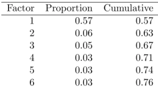
Table 3.1: Factors proportion of total variance Factor Proportion Cumulative

1 0.57 0.57 2 0.06 0.63 3 0.05 0.67 4 0.03 0.71 5 0.03 0.74 6 0.03 0.76

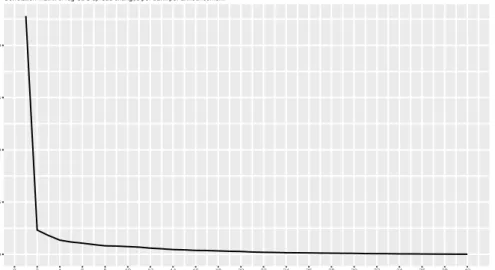
Table 3.1 shows us the first 6 factors and their respective proportion of the total variance explained. We conclude that one factor sufficiently explains 57% of the sample variance while estimating a model with two factors would only improve the explanatory power to 63% of total sample variance. Additionally, we can also visualize this with a scree graph, which is based on the eigenvalues in order to graphically determine the number of factors to include (Rencher,

(26)

Methodology

2002, p.426). The scree graph shows us that the size of the first eigenvalue (22,80) is substantially greater than the size of the following 39 eigenvalues. Taking into account this visual method, we also conclude that one factor should be sufficient.

0 5 10 15 20 0 2 4 6 8 10 12 14 16 18 20 22 24 26 28 30 32 34 36 38 40 Eigenvalue number Eigen value siz e

Correlation matrix of log CDS spread changes per bank per announcement

Scree graph

Figure 3.1: Scree graph of the eigenvalues

3.1.2 Principal component method and interpretation

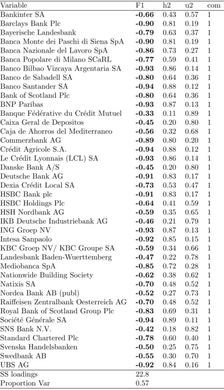
Now that we have determined the number of factors, we can proceed to estimate the correspond-ing factor loadcorrespond-ings. As mentioned in chapter 2, we will use the principal component method (Rencher, 2002, p.415). These factor loadings or factor weights reveal how much each banks’ in-dividual CDS return observation depends on the monetary policy factor. For a one-factor model, we estimate the factor loadings by multiplying the square root of the first eigenvalue with its corresponding eigenvector. We then obtain the factor loadings for each bank in our sample. Ta-ble 3.2 reports our factor estimates. We label our dominant factor as monetary policy. We can see that all banks load highly1 and negatively on the monetary policy factor. An increase of this factor corresponds with expansionary monetary policy measures, while a decrease corresponds with contractionary measures. This is derived from our estimated results that the factor and the bank CDS returns are negatively related, which aligns with the estimates of Boeckx et al. (2017); Altavilla et al. (2017), who found that unanticipated expansionary balance sheet mea-sures lead to a decrease in banks’ CDS spreads. The table also reports the communality (h2), which is the variance of the bank’s CDS return observation due to the common monetary policy factor. Consequently we also report the specific variance (u2), which the variance unique to each observation. The last column contains the complexity of the variable, which is the number

1_{As an arbitrary cut-off value, we chose a loading equal or greater than 0.30 to decide if a variable is associated}

(27)

Methodology

of factors a variable loads highly on. All variables report a complexity of 1, which means that we have obtained the simplest structure, that is when the variables have clearly been clustered into a group of one factor.

In addition, we provide our estimated factor loadings (column F1) from table 3.2 with an economic interpretation. Banks with factor loadings closer to -1 or 1 give us an indication that these are more correlated with the monetary policy factor than banks with factor loadings closer to 0. We have chosen an arbitrary value of 0.3 or higher to decide if a variable is associated with our factor (Rencher, 2002).

To further clarify the interpretation of this value, we compare Banco Santander (-0,94) with Caixa Geral de Depositos (-0,45). While both banks relate negatively to the monetary policy factor, the correlation of Banco Santander with the unobserved factor is stronger. However, this doesn’t necessarily imply that a decline in CDS returns of Banco Santander is roughly double the decline of Caixa Geral de Depositos because there is still a fraction of the CDS returns that is driven by banks specific components (the idiosyncratic error term ε in equation 2.8). In addition, values closer to -1 or 1 imply that the monetary policy factor explains a larger fraction in the variation of the change in bank CDS spread. For Banco Santander, 88% of the variation (communality) from the CDS return can be attributed to the monetary policy factor versus 20% for Caixa Geral de Depositos. This leaves us with 80% of the variation of Caixa Geral de Depositos unexplainable by the monetary policy factor.

Now that we have identified our monetary policy factor, we can go ahead and proceed to estimate the factor scores. We estimate these factor scores because we are interested in the behavior of the banks’ CDS return observations in terms of the monetary policy factor and not only in identifying the factor. We will report these estimates and plot them over the different announcement dates in the results chapter.

(28)

Methodology

Table 3.2: Estimated one-factor model

F1 = first factor, h2 = communality, u2 = specific variance

Variable F1 h2 u2 com

Bankinter SA -0.66 0.43 0.57 1

Barclays Bank Plc -0.90 0.81 0.19 1

Bayerische Landesbank -0.79 0.63 0.37 1 Banca Monte dei Paschi di Siena SpA -0.90 0.81 0.19 1 Banca Nazionale del Lavoro SpA -0.86 0.73 0.27 1 Banca Popolare di Milano SCaRL -0.77 0.59 0.41 1 Banco Bilbao Vizcaya Argentaria SA -0.93 0.86 0.14 1 Banco de Sabadell SA -0.80 0.64 0.36 1

Banco Santander SA -0.94 0.88 0.12 1

Bank of Scotland Plc -0.80 0.64 0.36 1

BNP Paribas -0.93 0.87 0.13 1

Banque Fédérative du Crédit Mutuel -0.33 0.11 0.89 1 Caixa Geral de Depositos -0.45 0.20 0.80 1 Caja de Ahorros del Mediterraneo -0.56 0.32 0.68 1

Commerzbank AG -0.89 0.80 0.20 1

Cr´edit Agricole S.A. -0.94 0.88 0.12 1 Le Cr´edit Lyonnais (LCL) SA -0.93 0.86 0.14 1

Danske Bank A/S -0.45 0.20 0.80 1

Deutsche Bank AG -0.91 0.83 0.17 1

Dexia Cr´edit Local SA -0.73 0.53 0.47 1

HSBC Bank plc -0.91 0.83 0.17 1

HSBC Holdings Plc -0.64 0.41 0.59 1

HSH Nordbank AG -0.59 0.35 0.65 1

IKB Deutsche Industriebank AG -0.46 0.21 0.79 1

ING Groep NV -0.93 0.87 0.13 1

Intesa Sanpaolo -0.92 0.85 0.15 1

KBC Groep NV/ KBC Groupe SA -0.59 0.34 0.66 1 Landesbank Baden-Wuerttemberg -0.47 0.22 0.78 1

Mediobanca SpA -0.85 0.72 0.28 1

Nationwide Building Society -0.62 0.38 0.62 1

Natixis SA -0.70 0.48 0.52 1

Nordea Bank AB (publ) -0.52 0.27 0.73 1 Raiffeisen Zentralbank Oesterreich AG -0.70 0.48 0.52 1 Royal Bank of Scotland Group Plc -0.83 0.69 0.31 1 Société Générale SA -0.94 0.89 0.11 1

SNS Bank N.V. -0.42 0.18 0.82 1 Standard Chartered Plc -0.78 0.60 0.40 1 Svenska Handelsbanken -0.50 0.25 0.75 1 Swedbank AB -0.55 0.30 0.70 1 UBS AG -0.92 0.84 0.16 1 SS loadings 22.8 Proportion Var 0.57

(29)

Methodology

3.2 Panel model

3.2.1 Panel data construction

The dependent variable in our model, ID CDS, consists of our estimated bank specific CDS reaction on a given policy date. We aim to explain this reaction with the most recent bank balance sheet and income statement data available to investors or regulators. As we are using year-end data, we explain the bank specific reaction based on explanatory variables from the year preceding the policy announcement. While we could have estimated a model over the individual daily reactions, we prefer not to because we would then have a whole year of policy announcements with constant bank business model variables. Instead we will first estimate a model where the bank specific CDS reaction is summed to a quarterly frequency to improve the variability of our panel. While quarterly data was made available to us in order to create a unique set of business model variables per quarterly observation, we opted to stick with the year-end data. Using quarterly data would have reduced our sample size to 19 banks instead of 40 because there was not sufficient data available for the banks of which we have estimated the idiosyncratic change in CDS returns. In addition, we will also estimate a model where we sum the idiosyncratic reaction to a yearly frequency so we can explain each idiosyncratic reaction with a unique set of business model variables. Our baseline model with a quarterly frequency consists of 1404 observations from 40 banks, the yearly frequency model consists of 349 observations from 40 banks. Note that our panel is an unbalanced panel, where the observation of the N individual banks are not observed in all T periods. While it would be an easy fix to simply discard the individual banks with missing observations and create a balanced panel, this could be highly inefficient due to the information loss (Verbeek, 2012, p.434). Nevertheless, because the observations are not systematically missing, we can still proceed with the unbalanced panel and obtain consistent and efficient estimators while including as much data as possible (Verbeek, 2012, p.434).

3.2.2 The fixed effects estimator

We first consider the fixed effects model where the intercept αi varies across the individual

banks. This would allow us to capture the bank specific features that are constant over time but not captured by our business model variables. In the simplest case, we could create a dummy variable for each bank in the cross section and include these as regressors . But because our sample consists of 40 banks, there would be too many regressors so we would then prefer to estimate a fixed effects model in deviations from their respective means (Verbeek, 2012,

(30)

Methodology

p.386). If we decide to use the fixed-effects estimator, our baseline model and the consistency assumptions would be the following:

ID CDSit− ID CDSi = (Xit− Xi)0β + (εit− εi), εit∼ iid(0, σ2ε) (3.1)

E[Xitεjs] = 0, ∀(i, j, t, s)

E[(Xit− Xi)εjs] = 0

3.2.3 The random effects estimator

If we choose the random effects model, we also let the intercept vary over individual banks but the crucial difference with fixed effects is that the individual effects are part of the error term. We can see that the error term consists of a bank specific component αi and an idiosyncratic

component εit. This implicates the use of the OLS estimator for random effects because the

error terms now show a structure αi. To deal with this autocorrelation, we could use generalized

least squares (GLS) which is a more efficient estimator (Verbeek, 2012, p.390).

ID CDSit= α + Xit0β + µit (3.2)

µit= αi+ εit, εit ∼ iid(0, σ2ε), αi ∼ iid(0, σ2α) (3.3)

E[αiεit] = 0, E[αiαj] = 0, ∀i 6= j

E[εitεis] = 0, E[εitεjt] = 0, E[εitεjs] = 0, ∀i 6= j, t 6= s

E[αiXit] = 0, E[εitXit] = 0

An important remark to make is that our sample is not randomly drawn, but rather based on availability of the data. This prompts us to be cautious with generalizing our results to the population distribution, in our case all European banks (Verbeek, 2012, p.394).

3.2.4 Fixed effects or random effects?

From an econometric point of view, our preference goes to random effects because it incorporates the within and between dimensions of our data and results in a more efficient estimator than the fixed effects estimator (Verbeek, 2012, p.394). The main condition for the random effects in order to be consistent is that the explanatory variables Xit should be uncorrelated with the individual

effects αi. If this is not the case, we would have to choose the fixed effects estimator which

remains consistent despite the correlated explanatory variables and individual effects. In order to determine the appropriate estimator, we will test for correlation between the explanatory variables Xit and the individual effects αi by making use of the Hausman test (Verbeek, 2012,

(31)

4 Results

4.1 Monetary policy stance identification

4.1.1 Estimated factor scores

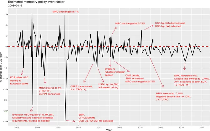
We will first discuss our estimates of the factor scores, by which we have measured the impact of the monetary policy factor from the different announcement dates on the change in bank CDS spreads. In order to explain which policy announcements had a greater positive or negative impact, we will visualize these factors over our sample period. For the more detailed output of estimates, we refer to the appendix (Table A.6).

−35 −30 −25 −20 −15 −10 −5 0 5 10 15 2008 2009 2010 2011 2012 2013 2014 2015 2016 2017 Year % c ha ng e ba nk C D S re tu rn 2008−2016

Estimated monetary policy event factor

Figure 4.1: Factor scores over time

On figure 4.1, we have highlighted the most important policy events that had a considerable impact on the bank CDS returns in our sample. The positive shocks correspond with restrictive monetary policy or policy inaction and lead to an increase in bank CDS returns, while negative

(32)

Results

shocks correspond with expansionary monetary policy measures which lead to a decrease in bank CDS returns by lowering the spreads. We will chronologically discuss some of the highlighted monetary policy events that had a noticeable impact on the bank CDS returns within our sample. During the global financial crisis, the main determinants driving CDS spreads were found to be individual liquidity, market liquidity and credit risk (Annaert et al., 2013; Chiaramonte and Casu, 2013). On the figure we see that three measures aimed at restoring liquidity on the interbank market and the individual banks, stand out within that period. The first 9% drop in CDS returns attributed to the monetary policy factor was on May 2, 2008 when the ECB offered USD liquidity to European banks in an attempt to improve liquidity in short-term USD funding markets (European Central Bank, 2008b). The second biggest drop within our sample was on October 13, 2008 following the announcement that the ECB would step up its efforts of providing USD liquidity ’as long as needed’, in cooperation with other central banks such as the Federal Reserve and the Bank of England (European Central Bank, 2008a). These tenders of USD funding had maturities varying between 1 week, 1 month and 3 months and were provided at fixed rates for full allotment. In essence, it was possible to borrow any amount at eased collateral requirements at times when liquidity on the interbank market was very low. These measures were reflected by a drop of 27,25% in bank CDS returns attributable to the policy factor. A third measure that stands out during the global financial crisis is the introduction of a 1 year LTRO and the first Covered Bond Purchase Programme (CBPP) which was designed to further ease funding conditions and improve liquidity on the covered-bond market (European Central Bank, 2009).

Alongside bank liquidity which remained significant after the sub prime crisis (Chiaramonte and Casu, 2013), an increasingly important determinant during the European debt crisis was sovereign risk (Drago et al., 2017), characterized by the sovereign-bank public debt connection. The bailout request by Greece on April 23, 2010 saw European bank CDS premia rise to un-precedented levels (Figure 2.1). The immediate impact of the policy announcement on May 10, 2010 resulted in the sharpest drop (34,47%) within our sample of bank CDS returns attributed to the monetary policy factor. During this event, the Securities Markets Programme (SMP) was announced alongside an arsenal of other liquidity measures such as 3 and 6 month LTRO’s and the reactivation of temporarily swap lines with the FED (European Central Bank, 2010). The immediate impact of the announcement was also well reflected by a sharp drop in yields, for example the spreads on the 10 year Greek bond vis-`a-vis the German bund decreased more than 400 bps (Manganelli et al., 2012). The Draghi speech on July 26, 2012 where he hinted about OMT, marked the start of a declining trend in Euro area bond yields (Alcaraz et al., 2018) and

(33)

Results

bank CDS spreads (Figure 2.1). We estimated a negative direct impact on bank CDS returns attributed to our monetary policy factor of 4,86% following his London speech. However, the policy announcement on August 2, 2012 where the MRO remained at 0,75% with no further measures, led to an increase of 5,2% in CDS spreads attributable to our policy factor. This could be an indication that the market expectations were not met due to the policy inaction. But the consecutive policy event on September 6, 2012 delivered with the reveal of the technical features of OMT which then resulted in a drop of 6,40% in bank CDS returns (European Central Bank, 2012).

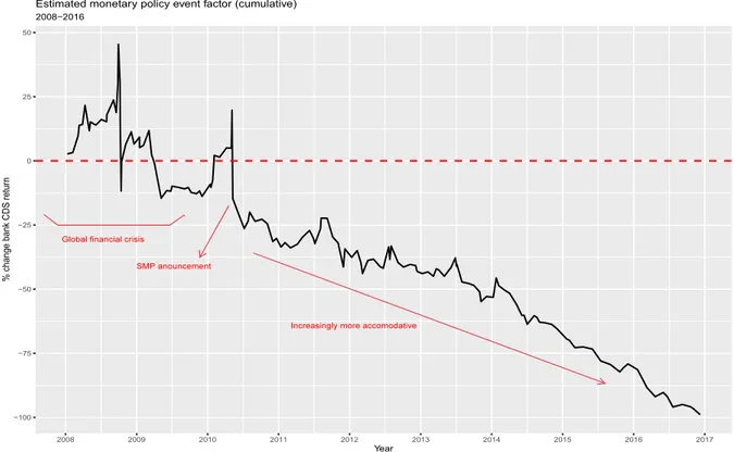
4.1.2 Cumulative estimated factor scores

Additionally, we have computed the cumulative impact of the monetary policy factor on bank CDS returns. This way we can identify the main monetary policy stance during sample period. For the more detailed output of estimates, we refer to the appendix (Table A.6).

−100 −75 −50 −25 0 25 50 2008 2009 2010 2011 2012 2013 2014 2015 2016 2017 Year % c ha ng e ba nk C D S re tu rn 2008−2016

Estimated monetary policy event factor (cumulative)

Figure 4.2: Cumulative factor scores over time

Figure 4.2 reveals that during the period of the global financial crisis, the cumulative impact of the ECB’s measures on bank CDS returns was briefly negative in the end of 2008 and the second half of 2009. This gives an indication that the ECB adopted an accomodative stance rather late into the financial crisis. Quite noticeably is the sharp drop since the announcement of the SMP, where the cumulative impact of the monetary policy factor on bank CDS returns

(34)

Results

became increasingly more negative. As mentioned earlier, this period is characterized mainly by very low policy rates, negative deposit rates, QE and extended liquidity provisions. This result is consistent with the findings of Altavilla et al. (2017), who estimated that following a period of accomodative monetary policy, banks experience a decrease in bank credit risk which is proxied by declining bank CDS spreads. Overall, we conclude that following the very accomodative monetary policy stance, the ECB has contributed to an improved perception of banks’ credit risk or in other words a lower perceived default probability of the banks in our sample.

4.2 Sensitivity of bank business models

4.2.1 Summary explanatory variables

Next to identifying the monetary policy stance of the ECB using bank CDS spreads, we are also interested in the bank business model determinants underlying the heterogeneous response to the different policy announcements. Table 4.1 summarizes our hypothesis of the different explanatory variables that represent the individual bank business models in our baseline model with their expected coefficient sign, which we explained more in detail back in chapter 2 along with the calculation methods.

Table 4.1: Variable description and expected sign

Variable Description Expected coefficient sign

CAP Ratio of equity to total assets -ROA Ratio of net income to total assets + / -LTA Ratio of net loans to earnings assets + / -DTL Ratio of deposits to liabilities -LLP Ratio of loan loss provisions to total loans + DIV Ratio of non-interest income to total revenue + / -Size Natural log of total assets

-4.2.2 Hausman test

In order to decide between the fixed effects and random effects estimators, we have performed the Hausman test (appendix table A.9). Our results indicate that we cannot reject the null hypothesis on the 5% significance level, and consequently opt for the random effects estimator because this will be consistent and more efficiently exploit the within and between dimensions of our panel data than the OLS estimates of the random effects model (Verbeek, 2012). The only downside of our choice from an economic point of view, is that our sample banks are not randomly drawn, but rather based on data availability and completeness. When interpreting the results, we will have to be cautious when generalizing.

(35)

Results

4.2.3 Whole sample estimation

Our estimation results of the random effects estimator are summarized in table 4.2. As previously mentioned, the first model consists of the idiosyncratic change in CDS spreads summed to a quarterly frequency, our second model contains the reaction summed to a yearly frequency. The explanatory power of our yearly model is greater than the quarterly model, which is not suprising because the yearly model tries to explain each individual idiosyncratic bank CDS change with a unique set of bank business models.

Table 4.2: Baseline estimation results

Dependent variable: ID CDS Random effects Quarterly Yearly (1) (2) CAP −0.037 −0.132 (0.167) (0.638) ROA 0.344 1.375 (0.590) (2.207) DTL −0.041∗ _−0.152∗ (0.022) (0.085) LTA 0.007 0.022 (0.024) (0.095) DIV 0.001 0.007 (0.017) (0.062) LLP 0.149 0.784 (0.438) (1.621) Size −0.820∗∗ _−3.326∗∗ (0.361) (1.422) Constant 18.080∗∗ 72.890∗∗ (8.219) (32.267) Observations 1,404 349 R2 0.011 0.044 Adjusted R2 0.006 0.025 F Statistic 16.016∗∗ 15.782∗∗ Note: ∗_p<0.1;∗∗_p<0.05;∗∗∗_p<0.01

Starting with our baseline models encompassing the whole sample period, the capital ratio appears to be statistically insignificant, but we find that the coefficient is negative. Using bank CDS spreads, we can only find weak support for the hypothesis that banks with higher capital ratios are less sensitive to monetary policy announcements (Madura and Schnusenberg,

(36)

Results

2000; Yin and Yang, 2013; Ricci, 2015). Additionally, our findings correspond with that of Altavilla et al. (2018), who concluded that the CDS of banks with lower regulatory capital does not increase following unexpected accomodative policy measures of the ECB. Furthermore this partially aligns with the findings of Ricci (2015), who investigated the determinants of different bank’s stock price reaction to ECB announcements. He found that the capital ratio was always insignificant for reactions to restrictive measures while only found to be significant for one event window of expansionary measures.

Next, the profitability measure ROA does not to appear to be statistically significant over the whole sample period but the positive sign aligns with the results of Ricci (2015) who found that more profitable banks reacted more to ECB policy announcements based on bank stock returns.

The DTL variable appears to be statistically significant on the 10% significance level, with a negative coefficient sign. Banks with a higher share of deposits in their funding are less sensitive to monetary policy measures of the ECB. This result supports the findings of (Yin and Yang, 2013; Ricci, 2015) who argue that extensive use of non-deposit funding increases the exposure of banks to monetary policy interventions. Additionaly this finding is supported by one of the main determinants driving CDS spreads during our sample period, which is individual liquidity (Annaert et al., 2013; Chiaramonte and Casu, 2013; Drago et al., 2017).

Furthermore, we find a positive coefficient for LTA and DIV, but both appear to be in-significant. We thus find no conclusive evidence that non-traditional banking activities increase the exposure to monetary policy shocks. While credit risk is a determinant driving bank CDS spreads (Annaert et al., 2013), our results do not strongly reflect this because we find an in-significant but positive coefficient for our variable LLP. We can thus only find weak support for the hypothesis that banks with a higher share of loan loss provisions react more sensitively to monetary policy announcements based on CDS spreads.

At last, we find that Size, the log of the bank’s total assets, is significant on the 5% significance level and has a negative coefficient. This supports the hypothesis that larger banks in our sample react less to monetary policy measures of the ECB. One possible explanation for this is that small banks are found to increase new loans to high-risk borrowers following expansionary monetary policy shocks, while the risk exposure of large banks remains unchanged (Buch et al., 2014). In addition, because our sample period consists of a broad set of non-conventional measures and a steady decrease of interest rates towards the zero lower bound, large banks are found to better preserve their net interest margins in extended periods of expansionary monetary policy measures (Buch et al., 2014; Lamers et al., 2019).

(37)

Results

4.2.4 Robustness over subsamples

In addition, we investigate how our model performs during different subsamples. We proceed by estimating our two baseline models seperatly during the global financial crisis (2008-2009), soverign debt crisis (2010-2012) and post-crisis period (2013-2017). This allows us to check our results under varying macroeconomic environments. Moreover as mentioned earlier, the determinants driving bank CDS spreads are found to be time-varying (Annaert et al., 2013; Chiaramonte and Casu, 2013). The results reported in table 4.3 are from the random effects estimator, the Hausman tests for these specifications can be found in the appendix (Table A.10).

Table 4.3: Subsample estimation results

Dependent variable: ID CDS Random effects

Quarterly Quarterly Quarterly Yearly Yearly Yearly 2008-2009 2010-2012 2013-2017 2008-2009 2010-2012 2013-2017 (1) (2) (3) (4) (5) (6) CAP −0.514 0.131 −0.122 −2.153 0.523 −0.563 (0.628) (0.199) (0.129) (2.364) (0.671) (0.496) ROA 1.718 −0.629 0.728 7.012 −2.515 3.588∗∗ (2.190) (0.704) (0.489) (8.149) (2.371) (1.802) DTL −0.151∗ −0.040 −0.011 −0.607∗∗ −0.158∗ −0.032 (0.079) (0.027) (0.015) (0.298) (0.089) (0.059) LTA −0.005 0.021 0.023 −0.025 0.086 0.078 (0.081) (0.027) (0.018) (0.304) (0.091) (0.072) DIV 0.016 −0.014 0.013 0.067 −0.055 0.059 (0.052) (0.022) (0.013) (0.192) (0.074) (0.049) LLP 1.704 0.246 −0.316 7.303 0.983 −0.677 (2.089) (0.535) (0.320) (7.819) (1.800) (1.187) Size −2.074 −0.067 −0.748∗∗∗ _−8.489∗ _−0.269 _−3.142∗∗∗ (1.296) (0.444) (0.242) (4.903) (1.494) (0.971) Constant 47.107 2.006 15.205∗∗∗ 192.495∗ 8.025 63.507∗∗∗ (28.862) (9.834) (5.688) (109.075) (33.105) (22.678) Observations 312 468 624 78 117 156 R2 _0.027 _0.016 _0.068 _0.120 _0.087 _0.234 Adjusted R2 _0.004 _0.001 _0.058 _0.032 _0.029 _0.197 F Statistic 8.284 7.390 45.104∗∗∗ 9.535 10.435 45.107∗∗∗ Note: ∗p<0.1;∗∗p<0.05;∗∗∗p<0.01

First off all, we notice that the explanatory power of our yearly model during the post-crisis period (2013-2017) is the highest. Our subsample estimation results reveal that the capital

(38)

Results

ratio remains insignificant in explaining the individual banks reaction to ECB monetary policy announcements with the coefficient signs varying over the different periods. We cannot find conclusive evidence using bank CDS spreads in favor of the hypothesis that bank’s with higher capital ratios are less exposed to monetary policy announcements.

The coefficient of our profitability measure, ROA, is insignificant in all periods except for our yearly model during the post-crisis period where the coefficient is positive and significant on the 5% significance level. Using bank stocks, Ricci (2015) found similar results, indicating that the more profitable banks in our sample reacted more to ECB events during this window. A possible explanation for this finding could be that this period was characterized by expansionary measures lowering the interest rate to the zero lower bound, which put pressure on the profitability of banks. Increased profitability would then be a reflection of shifting part of their lending to more risky borrowers. Additionally, Buch et al. (2014) found evidence that following expansionary measures in a low for long environment, banks tend to increase their risk exposure.

Next, the negative coefficient of DTL appears significant for both models during the global financial crisis period and for the yearly model during the sovereign debt crisis. This again confirms our results that the banks in our sample with more non-deposit funding have a higher exposure to monetary policy announcements, especially during periods of severe pressure on financial markets and a deteriorated macroeconomic environment. Furthermore, we were unable to find conclusive evidence that LTA, DIV or LLP affect the CDS reaction of banks in our sample to ECB policy announcements as all coefficients were found to be statistically insignificant.

Lastly, we find that the negative coefficient of bank size is significant in the yearly model during the global financial crisis and in both models during the post-crisis (2013-2017). This again supports our hypothesis that larger banks in our sample react less to monetary policy announcements of the ECB, especially during our post-crisis period.

To summarize our main results, we were unable to find evidence that the banks in our sample with lower capital ratios reacted more to monetary policy surprises of the ECB, based on the bank specific CDS returns. Secondly, we showed that the ratio of deposits to liabilities is an important determinant in the response of the bank CDS to monetary policy measures, especially during the financial crisis and sovereign debt crisis. At last, we find that there could be increased risk taking following a period of extended monetary policy easing. This is reflected by the idiosyncratic CDS return of banks in our sample with a lower asset size and higher ROA responding more sensitively to the ECB’s monetary policy measures, especially between 2013 and 2017.