Analysis and optimization of 3D renal
anatomy reconstruction for
Robot-Assisted Partial Nephrectomy planning
Maryse Lejoly
Student number: 01407717
Stefanie Vanderschelden
Student number: 01508793
Supervisor(s): prof. dr. Karel Decaestecker, dr. Pieter De Backer, prof. dr. ir. Charlotte
Debbaut
A dissertation submitted to Ghent University in partial fulfilment of the requirements for the
degree of Master of Medicine
Universiteitsbibliotheek Gent, 2021.
This page is not available because it contains personal information.
Ghent University, Library, 2021.
PREFACE
For this master dissertation, we were brought together after both choosing this subject. We chose this subject because it consisted of a collaboration with engineering students. It turned out really interesting working with them by obtaining more insights in this part of medicine. Their expertise has made a major contribution to this master dissertation. So we would like to especially thank Sarah Vandenbulcke, Jordi Martens and Saar Vermijs.
We also would like to address a big word of gratitude towards dr. Pieter De Backer, who gave us excellent guidance during the entire process, as well as insights and constructive feedback.
Thanks to the Mimics team we learned to master Materialise Mimics. And for the radiological part, we would like to thank Pieter De Visschere, who gave us advice hereabout. Also, regarding the radiology, we would like to thank dr. Mottrie, dr. De Naeyer and dr. Claus from the OLV hospital located in Aalst, who we owe the CT data to.
Furthermore, this master dissertation would not have been possible without professor. dr. Karel Decaestecker and professor Charlotte Debbaut. We would like to thank them for the constructive feedback. Prof. dr. Karel Decaestecker also gave us the opportunity to attend a partial nephrectomy surgery, it was a really good experience.
This means the end of the theoretical part of our study, so we are going to take this opportunity to thank the people who helped us get where we are today: our parents, our brothers and sisters and Mr Louis Deconick. Lastly, we would like to thank Wolf Kriauciaunas for proof-reading.
Stefanie Vanderschelden and Maryse Lejoly December 2019
LIST OF FIGURES
Figure 1 Graves classic description of renal vascular segmentation (10).
Figure 2 Anatomy of the left renal artery. Extra- and intraparenchymal arterial sections are distinguished. Courtesy of V. Ficarra, university of Udine and V. Macchi, University Padua (13).
Figure 1 Anatomical variations. Left: a real aneurysm, middle: multiple micro-aneurysms, right: fibromuscular dysplasia adapted from Harrison et al. (8).
Figure 2 1 - USAT1, 2 - USAT2, 3 - USAT3, 4 - USAT4, USAG1 in frame USAG2 out frame, A - renal artery, B - anterior division, D - upper segmental artery, E - middle segmental artery, F - apical segmental artery, G - ureter, H - Pelvis, I - upper major calyx, J - lower segmental artery adapted from Mishra et al. (1).
Figure 3 Two head renal arteries (a), polar arteries (b and c), early bifurcation (b) adapted from Dani et al. (19).
Figure 6 Late confluence - Multiple veins - Circumaortic veins - Retroaortic veins addapted from Famurewa et al. and Sebastia et al. (16,21).
Figure 7 Prevalence of collateral arterial blood supply vessels in the different parenchymal segments defined according to Graves classification (23). Figure 8 Stages of renal cancer (27).
Figure 9 Polar lines RENAL/PADUA (32). Figure 10 Centrality Index (50).
Figure 11 Triangles (radius of tumor), squares (distance) (50).
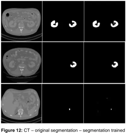
Figure 12 CT – original segmentation – segmentation trained model (55). Figure 13 Summary of the process (56).
Figure 14 Comparison of the Visible Patient© tool (left) and the tool from this study (middle) and the 3D model as segmented by M. Lejoly/S. Vanderschelden (56).
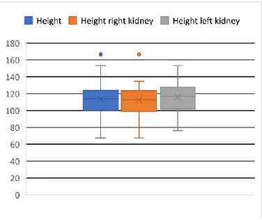
Figure 15 Superior pole versus inferior pole thickness. Figure 16 Boxplot height right kidney vs height left kidney. Figure 17 Circle diagram: USAT types.
Figure 18 Example measurement of distance before first division (green line) using Mimics.
Figure 20 Circle diagram: multiple arteries.
Figure 21 Frequency of planned PN and RN per PADUA score. Figure 22 Frequency of planned PN and RN per RENAL score. Figure 23 Frequency of planned PN and RN per C-index. Figure 24 Scatter graphic comparing C index to PADUA score. Figure 25 Scatter graphic comparing C index to RENAL score. Figure 26 Scatter graphic comparing PADUA score to RENAL score.
Figure 27 Arteries at the beginning of the thesis and after training with mimics and the difference in regions + Visible Patient arteries (right).
Figure 28 Second model, after training with Mimics, compared to Visible Patient© model.
LIST OF TABLES
Table 1 TNF classification based on adapted from EAU guidelines (26). Table 2 TNM stage grouping adapted from EAU guidelines (26).
Table 3 Proposed surveillance schedule following treatment for RCC (CT = CT of chest and abdomen with MR for abdomen as an alternative, US = US of abdomen, kidneys and renal bed) adapted from (26).
Table 4 PADUA vs. RENAL score (49). Table 5 Legend Mimics.
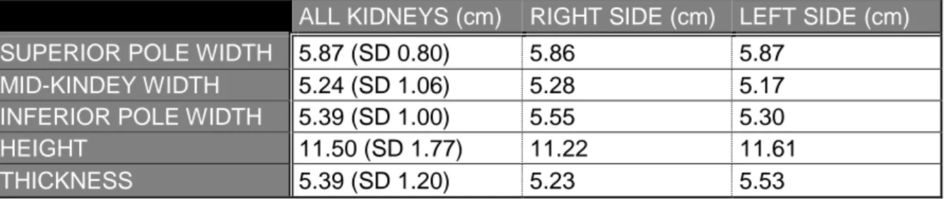
Table 6 Measurements of kidneys during this study.
Table 7 Distribution of USAT: comparison between this study and Mishra et al. (1).
LIST OF ABBREVIATIONS
ACR American College of Radiology
CI Centrality-Index
CKD Chronic Kidney Disease
CT Computer Tomography
CV Cardiovascular
CVE Cardiovascular Event
EAU European Association of Urology (e)GFR (estimated) Glomerular Filtration Rate
HU Hounsfield Units
ICC Interclass Correlation Coefficient
ICG Indocyanine Green
IVC Inferior Vena Cava
MR Magnetic Resonance
NCCN National Comprehensive Cancer Network OPN Open Partial Nephrectomy
PADUA Preoperative Aspects and Dimensions Used for an Anatomical
PN Partial Nephrectomy
RALPN Robot-Assisted Laparoscopic Partial Nephrectomy RAPN Robot-Assisted Partial Nephrectomy
RCC Renal Cell Carcinoma
RENAL Radius, Exophytic/Endophytic, Nearness, Anterior/posterior, Location
RN Radical Nephrectomy
SD Standard deviation
TNF Tumor Nodes Metastasis
US Ultrasound
TABLE OF CONTENTS
Abstract (English) ... 1
Abstract (Dutch) ... 2
Chapter 1: Introduction ... 3
1. Goal of the dissertation ... 3
Chapter 2: Physiological and pathological renal anatomy ... 4
1. History ... 4 2. Embryology ... 4 3. Kidney proportion ... 5 4. Physiologic vascularization ... 5 5. Anatomical variations ... 7 5.1 General arteries ... 7
5.2 Superior segmental A. renalis ... 8
5.3 Number of Aa. renales and early division ... 9
5.4 General Veins ...10
5.6 Tumor vascularization ...11
Chapter 3: Kidney cancer ...13
1. Symptoms ...13 2. Diagnostics ...13 3. Treatment ...13 3.1 TNF Classification ...14 3.2 Guidelines in TNF context ...15 3.2.1 Stage I, pT1 ...15
Operative therapy: Partial nephrectomy ...15
Non-surgical therapy ...16
Ablation therapy ...16
3.2.2 Stage II, pT2 ...16
3.2.3 Stages III and IV ...17
Operative therapy: Radical nephrectomy ...17
3.2.4 General ...17
3.2.5 Follow up ...17
3.3 Open vs Laparoscopic vs and Robot assisted approach ...18
3.3.1 Differences in outcome ...20
3.3.2 Procedural steps in RAPN ...21
3.3.3 Clamping...22
Chapter 4: 3D modeling ...28
1. Automatic segmentation ...28
2. Renal perfusion model ...30
Chapter 5: Materials and methods ...32
1 Materials ...32
Scanning protocol ...32
Patient-specific factors ...33
Mimics Research 21.0© experience...33
2 Methods ...34
Chapter 6: Results ...35
1.Renal parenchyma ...35
2.Vascularization ...36
3.Tumor ...38
4. Influence of segmentation quality ...41
5. Image from operation ...42
Chapter 7: Discussion ...43
1. Parenchyma ...43
2. Vascular ...43
3. PADUA, RENAL, Centrality index – tumor ...45
Chapter 8: Conclusion ...46
Chapter 9: Outlook ...47
References ...48 Addendum 1 ... I Addendum 2 ... X
Abstract (English)
Approximately 400.000 people are diagnosed with kidney cancer worldwide every year. One of the therapy options to treat early-stage kidney cancer (T1a tumors) is Robot-Assisted Partial Nephrectomy (RAPN). In this nephron-sparing surgery, only part of the kidney is resected. The surgery is often performed through selective clamping: only the arteries going towards the tumor are clamped so the blood flow to the tumor is interrupted and a bloodless tumorectomy becomes theoretically possible, whilst keeping the healthy renal tissue perfused all the time. Good knowledge of the anatomy of the kidney and its vascularization is important to decide which arteries to clamp and clip. Until now the surgeon based his/her decision on CT scans. To facilitate this decision, 3D models could be useful. This master dissertation examines the vascularization of the kidney and all its variations. Next, 3D models of 67 kidneys including arteries, veins, tumor and urinary tract, were made using Mimics Research 21.0 by Materialise (c).
A first step towards comparing virtual pathological renal anatomy on anonymous patients to the physiological kidney anatomy from cadaveric studies was performed. Regarding the comparison in sizes of the kidneys, this research shows that the presence of a tumor has little impact. But when considering the vascularization more variations can be found in the oncological setting. In addition to the anatomy, three preoperative score systems were compared: PADUA score, RENAL score and Centrality-Index. It was found that the PADUA and RENAL scores are mostly similar. Both hard to calculate without 3D model, yet their outcome is more accurate in deciding between PN and RN than the Centrality-Index.
The models, made for this research, also serve as a database for an engineering algorithm which will automatically predict renal perfusion. We provide a tutorial on how to generate a 3D kidney model and show retrospective use cases of technology.
Abstract (Dutch)
Bij benadering 400.000 mensen worden wereldwijd jaarlijks gediagnostiseerd met nierkanker. Eén van de therapeutische opties in de behandeling in een vroeg stadium (T1a tumoren) is de Robot Geassisteerde Partiële Nefrectomie, beter bekend als Robot Assisted Partial Nephrectomy (RAPN). Gedurende deze nefron-sparende operatie wordt slechts een deel van de nier weggesneden. Terwijl ondergaat ook slechts een deel van het niervolume ischemie zodat de rest van de nier tijdens de gehele procedure zijn functie kan behouden. Dit wordt bekomen door het zeer selectief klippen van de arteriën: enkel de arteriën die rechtstreeks de tumor en omliggend nierparenchym bevloeien, worden dichtgehouden door middel van een clip zodat ze niet langer bevloeid worden. Op deze manier kan een tumorectomie theoretisch gezien zonder bloedverlies verlopen terwijl het gezonde nierweefsel de hele tijd bevloeid wordt. Een goede anatomische kennis van de nier en zijn bloedvaten wordt hier dus voor vereist om te beslissen welke bloedvaten al dan niet tijdelijk moeten onderbroken worden. Tot op vandaag maakte de opererende arts deze keuze aan de hand van CT scans, maar deze keuze zou kunnen vergemakkelijkt worden door het gebruik van 3D modellen. Deze thesis onderzoekt de vascularisatie van de nier met al zijn variaties. 3D modellen van 67 nieren werden hiervoor gemaakt met onder meer ook de renale arteriën, venen, tumor en urineweg. Hiervoor werd Mimics Research 21.0 van Materialise© gebruikt.
Een eerste stap werd gezet in het vergelijken van virtuele, pathologische nierpathologie op anonieme patiënten met de fysiologische nierpathologie van studies omtrent kadaveranatomie. Bij het vergelijken van de maten van de nieren, toonde dit onderzoek dat de aanwezigheid van een tumor slechts een kleine impact had hierop. Echter, wanneer er gekeken wordt naar de verschillen in vascularisatie kunnen meer variaties gevonden worden bij oncologische dan bij fysiologische nieren. Buiten deze anatomische vergelijking werden er ook drie preoperatieve score systemen onder de loop genomen: de PADUA score, de RENAL score en de C-Index. In de uitkomst bleken de PADUA en RENAL score voornamelijk gelijkaardig te zijn. Beiden zijn wel moeilijker te berekenen zonder 3D model, maar ze zijn accurater bij het beslissen tussen een partiële of een radicale nefrectomie dan de C-Index. De modellen, gecreëerd gedurende dit thesisonderzoek, diende ook als een database voor ingenieursstudenten. Zij werkten aan een algoritme dat automatisch renale bevloeiingskaarten kan voorspellen. Verder werd in deze studie een handleiding afgewerkt i.v.m. de manier waarop een 3D model gemaakt kan worden en worden er enkele technische toepassingen van de modellen aangehaald.
Chapter 1: Introduction
1. Goal of the dissertation
Every year approximately 400,000 people are diagnosed with kidney cancer worldwide. In 2018 alone, 254,507 men and 148,755 women were diagnosed and in 175,098 patients this was the primary cause of death (1,2). The etiology is rather uncertain but aging, obesity, greater adult attained height and high blood pressure are certain risk factors (3). Hence, these numbers will only increase because of global aging and the often unhealthy standard of living of the “Western” population. People with an age between 50 and 70 and men are more likely to be affected.
Kidney cancer is a fast-growing cancer type. In the onset, the disease has few symptoms leading to the issue that the diagnosis is often made late. But if the tumor is detected in an early stage, often by coincidence, there is a 79 to 100% chance of cure (4–6).
The most recent therapy of kidney cancer is Robot-Assisted Partial Nephrectomy (RAPN). During each operation it is of major importance that the individual vascular structures are well known by the surgeon, considering it reduces the risk for more blood loss and other complications, as well as the operating time. The surgeon must pursue to keep operating time as low as possible because when exceeding 25 minutes, an added 5 to 6% of risk of damage to the renal tissue was found (7). Also, it is required to know the individual anatomy of the kidney when dealing with portal hypertension, vascular anomaly of the aorta and aneurysm of the abdominal aorta (8).
In this experimental study is to chart the anatomy of the kidney and its tumors. In addition, we will also check if the finished 3D virtual models correspond to the anatomical properties derived from cadaveric studies. Three research questions will be answered during this dissertation: is there a relation between the sizes produced by this study and the ones found in other anatomical studies? Does the presence of a tumor influence the vascularization, again found in previous anatomical cadaveric studies? What is the current most useful preoperative classification system (PADUA, RENAL, C-Index)?
Additionally, the purpose is to finally work towards a tool, cooperating with engineering students, that will assist the surgeon in RAPN. This tool should be able to automatically make patient-specific 3D structures from their Computed Tomography (CT) scans and calculate which artery irrigates each kidney volume (whether or not tumor volume). This way the surgeon can decide in advance with more certainty which arteries should be clipped for having the least
possible blood loss while maintaining perfusion to the largest possible kidney volume during the whole procedure.
Chapter 2: Physiological and pathological renal
anatomy
1. History
Due to its complexity, the anatomy of the renal vasculature has been studied for centuries. The first hypothesis, stating renal compartmentalization in segments according to its arterial supply, is traced back to 1744, by Hunter and Brodel (1). This theory was confirmed by Hyrtl (9) later on in 1882, he described the renal arteries as end vessels, making the kidney particularly sensitive to ischemia. Graves was the first to describe the segmentation of the renal vascularization with its possible variations in 1954. He divided the kidney into five segments (1,9,10). Kher (1) further explored the renal segmentation in 1960 and Sykes described its relation with the tubules in 1964, while Verma (1), Saxena (1), Longia (1) and Ajmani (1) studied branching patterns and vascularization (1,9,10).
2. Embryology
The kidney is a structure consisting of approximately 1,000,000 nephri, it’s functional units (11). The organogenesis starts as with any organ at the three germ leaves. The kidneys originate from the intermediate mesoderm. The nephrogenesis itself begins in the 4th week. At a first stage, a pronephros, a structure consisting of one single nephron, is formed. It will, later on, be replaced by mesonephri, a structure consisting of multiple nephri, which will turn out to become the definitive kidney, called the metanephros (12). Starting from week six, the metanephros ascends from the pelvis through the abdomen to the lumbar area until it meets with the adrenal. The right kidney will stop ascending 1-2cm lower than the left one because of the location of the liver so that the kidneys are located on the psoas and quadratus lumborum muscles. The posterior surface of the right kidney is crossed by the 12th rib, and the left kidney by the 11th and 12th rib. The upper pole of the kidney is facing more medially in comparison with the lower pole. During the process of ascending the kidney generates arteries but meanwhile the lower arteries atrophy. This way the right artery will be longer than the left one because it has to cross the Inferior Vena Cava (IVC) on its posterior side. Errors during the vascularization process result in the growth of accessory arteries as discussed below (2,13– 15).
The origin of the urinal drainage system starts in the fifth week after fertilization when the metanephros is forming. From the lower part of Wolff’s duct appears a bud that is called the nephrogenic diverticulum. This bud grows cranially and will become the urinary tract. Later on, it will debranch in the collecting tubes and will become the pyelum and its chalices.
The metanephros is a working organ (in contrast to a pronephros) and can produce urine, which will be an important component of the amniotic fluid which is necessary for the growth of the fetus (16).
3. Kidney proportion
In general, there is a significant correlation between kidney length and the length of the individual itself. The left kidney is both in fetal as in adult kidneys larger than the right one. The length of the left kidney numbers 11.21 cm on average towards 10.97 cm in the right kidney. The thickness at the hilum numbers 3.37 cm on the left and 3.21 cm on the right kidney on average. The width of the kidney is larger on the superior pole (the mean is 6.48 cm) than on the inferior pole (mean is 5.39 cm) (14).
4. Physiologic vascularization
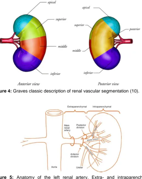
The kidney can be divided into five segments: four anterior segments (apical, superior, middle and inferior) and one posterior segment (1,9,10). Graves was the first one to describe the arterial vascularization of these five segments. At the time open nephron-sparing nephrectomy with hilar occlusion en bloc was performed with cold ischemia. The clinical relevance of abnormalities in the microvascular segmentation was not clear, this is why variants in the arterial tree were not well described. 42% Of the population has renal vasculature concomitant with Graves’ theory (10).
The Aa. renales originate at the height of lumbar 1-2 from the aorta descends lateral on both sides, just inferior to the origin of the A. mesenterica superior (1). The main A. renalis branch has a normative length of 4-6 cm and a diameter of 5-6 mm, although these normative diameters only apply to a quarter of the population (15). More distally, the arteria splits in an anterior and posterior branch. The anterior branch has the highest flow as it perfuses four of the five segments, which translates into 75% of the renal artery output. Whereas the posterior branch will only provide the posterior segment, accountable for 25% of the renal artery output (9). In terms of the renal veins, it is important to know that they are parallel to the arteries and usually located on their anterior side (16). Venous anatomy is discussed in paragraph 5.4. Major segmental branches of the renal artery and major tributaries of the renal vein are
positioned on the anterior surface of the renal pelvis. Infundibular arteries and veins course parallel to the upper-pole infundibulum, anterior and posterior (14).
Figure 4: Graves classic description of renal vascular segmentation (10).
Figure 5: Anatomy of the left renal artery. Extra- and intraparenchymal arterial sections are
distinguished. Courtesy of V.ficarra, University of Udine and V. Macchi, University Padua (13). The anterior-posterior transition is characterised by an avascular frontal plane that is being defined by the so-called Brödels line. This line is rather theoretical and is not being used for surgical planning. The only present anastomoses are found in the 4th and 5th generation arteries, meaning the vessel after the 3rd and 4th arterial branching, as described by Macchi et al. (17) in 2018. In all their studied subjects, they found crossing vessels in the middle segment and sometimes also in the inferior or superior segment. In general, the avascular plane is located medially from the lateral convex edge of the kidney and the mean distance until the lateral edge amounts 2,04 cm (17).
5. Anatomical variations
5.1 General arteries
A lot of anatomical variations in arterial trees exist. Proposed percentages differ amongst studies. As mentioned before, it is estimated that only 42% of the population has normal renal anatomy according to Graves as indicated by Borojeni et al. (9). The study of Famurewa et al. (16) in a Nigerian population states variation in 50% whereof 37% is arterial and 13% venous (16). This corresponds to the study of Munnusamy (2) showing 51% variation. Here the main focus went to early division and accessory arteries originating from the aorta (2). However, Macchi et al. (17) found that this would only be the case in as little as 13% of the population (17). And Mishra et al. (1) claim that in most cases, the abnormality can be found at the level of the segmental arteries (1).
In terms of artery size, we see that 25% of the population has a main renal artery with a length variating between 4 to 6 cm and a diameter variating between 5 to 6 mm. So, it is clear that there is a need for uniform criteria to describe the variances. Yet, in general, the variation percentage is thought to be somewhere around 50% (2,8,13,16).
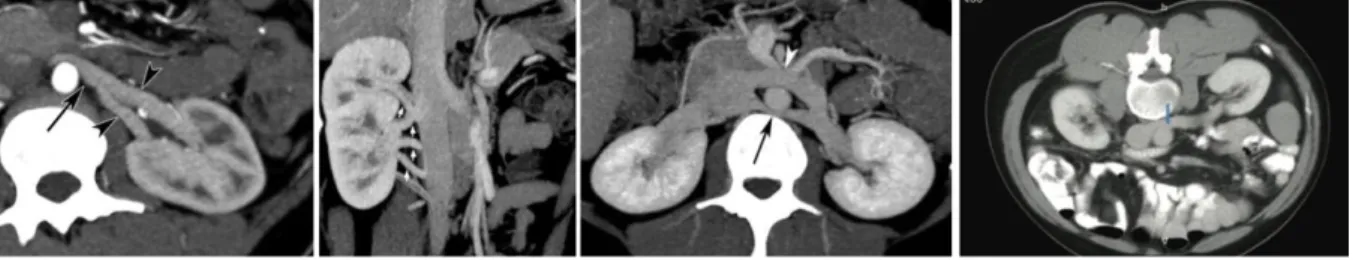
Variations in vascularization can be categorized by origin, caliber, relationship and obliquity. For example, looking at the origin, it shows that 92% of the main renal arteries insert lateral, 6% anterolateral and 2% posterolateral on the aorta in the region of L1-L2 (2). Variation can also be discussed by the shape of the renal artery. In the study of Harrison et al. (8), following variations can be categorized: significant stenosis of A. renalis (2%), fibromuscular dysplasia (2%), micro aneurysms (0.5%) and real aneurysms (1%). Figure 3 shows those variations (7).
The amount of abnormalities is significantly higher in the male gender, with horseshoe kidney (the two kidneys are fused together) as a particular example (16). This without a clear
explanation. The awareness of this is clinically important because men are more likely to be affected by terminal renal disease and hence are more likely candidates for kidney
transplants (18).
Figure 6: Anatomical variations. Left: a real aneurysm, middle: multiple micro-aneurysms, right:
Social, ethnic and racial differences also have their influence when talking about kidney variation, e.g. there is assumed to be more variation in the African than the Indian population (2).
5.2 Superior segmental A. renalis
In 2015 Mishra et al. (1) describes four anatomical variations in the origin of the superior segmental renal artery. 50 human kidneys (30 male and 20 female) obtained from postmortem bodies within 24 hours after death, where observed by corrosion cast method in 2009-2010. The minimum and maximum ages were respectively 18 and 60. When there were signs of renal trauma, renal pathology or decomposition the kidney was excluded. This study was done at Sarojini Naidu Medical College, a college in India. The following types were described: (1) USAT1: this model follows the normal vasculature, described by Graves. The superior segmental artery originates from the anterior part of the renal artery. This most frequent type with a prevalence of 40%. This percentage correlates with the 42% in the study of Borojeni et al. (1,9).
USAT2: The superior segmental artery originates from the middle segmental artery. The prevalence is 28%.
USAT3: The superior segmental artery originates from the apical segmental artery in 20% of the study cases. However, in other studies, this percentage is much higher, as it surpasses the frequency of USAT1 making it the most frequent subtype. It is important to recognize this type of variation because when clamping this apical vessel, there is a risk of ischemia in the superior segment.
USAT4: In 10% of the cases, the superior segmental artery originated from the posterior branch of the renal artery.
And finally, 2% of the cases had a total absence of the superior segmental renal artery (1). These four types are finally divided into two groups: on the one hand USAG1 where the artery lies in front of the upper major calyx, accounting for 80% of the cases and on the other hand USAG2 containing the other 20% where the artery is located medial when going towards the pelvis and the upper major calyx (1).
5.3 Number of Aa. renales and early division
At the level of the main renal artery, the following deviations have been described.
Borojeni et al.(9) describe one single renal artery in 75% of the cases. In 22% a polar artery was also present and in the remaining 3% two head renal arteries were found. Head renal arteries are defined as two renal arteries travelling from the aorta to the hilus while a polar artery is travelling directly towards the upper or lower pole of the kidney (see figure 5) (9,10,15). Klatte T. et al. (13) indicates that a double renal artery is more common on the right side. These numbers resemble those of Welds et al. (10) in 2005, apart from the higher frequency of two head renal arteries (12.3%). Welds et al. (10) found that 24.7% of the patients had a polar artery (9,10). Those numbers were very similar to the study of De Mello et al. (15) in 2016 who reported one single arteria renalis in 62.49% in the right kidney and 72.50% in the left kidney (15).
Figure 7: 1 - USAT1, 2 - USAT2, 3 - USAT3, 4 - USAT4, USAG1 in frame USAG2 out frame, A - renal
artery, B - anterior division, D - upper segmental artery, E - middle segmental artery, F - apical segmental artery, G - ureter, H - Pelvis, I - upper major calyx, J - lower segmental artery adapted from Mishra et al. (1).
Figure 8: Two head renal arteries (a), polar arteries (b and c), early bifurcation (b) adapted from Dani
et al. (19).
Looking at Munnusamy et al. (2) in the Indian population even higher numbers were found: in 38% more than one renal artery originated from the aorta, no distinction was made between a polar renal artery and a second head renal artery. However, a possible selection bias in terms of the population is possible. In India, it is more common to marry a relative. Because of the incest, the frequency of variations could be higher. Only in 49% of the study population, one single (“normal”) artery was seen. In this study, another variation has been taken into consideration, namely an early division of the head renal artery. An early division means that the main renal artery splits for the first time after less than 1 cm distal to its origin in the aorta (15). This was seen in 13% of the cases (2). De Mello et al. (15) described this variation in only 0,5%. Famurewa et al. (16) reported early divisions in the right kidney in 4% of the cases and in the left kidney in 0,5% of the cases. The higher frequency in Munnusamy et al. (2) could again be linked to incest. Also, variation is seen more frequently on the right side (25%) than on the left side (1%). On the one hand, more deviations on the left would be expected due to the longer ascend of the left kidney. On the other hand, more variations are seen on the right side. Probably because the arteries that are formed during the ascending have to be formed closer to each other and leaving them less space.
Further, the chances are greater to have a variation when there is already another anomaly present contralateral (8,15,16). Knowing that on the right side the renal artery originates posterior to the IVC, an early bifurcation is not easily visually differentiable from two separate renal arteries. Therefore, the surgeon must treat both cases as two different renal arteries because on this side, there is a higher risk of damaging the IVC (15).
5.4 General Veins
As expected, the renal venous system also shows quite some variations. However, these deviations are rare and location dependent. These variations can be a late confluence (right 3%, left 2,5%), multiple veins (right 2.5%, left 2.5%, total 5%), circumaortic veins, retro-arctic veins (2%). Harrison et al. (8) describe different numbers for multiple veins. On the left side always only one vena renalis is seen and on the right side, there are two to three renal veins in 30% (8). Molema et al. (20) even describe multiple veins up to 40% on the right side (20).
A late confluence means that multiple vein branches assemble within 1.5 cm from the IVC on the right or 1.5 cm of the lateral margin of the abdominal aorta on the left. Multiple veins are more than one vein draining directly into the IVC. A circumaortic vein is a left renal vein who is divided into an anterior and a posterior branch that encircles the abdominal aorta. And a retroaortic vein is a left renal vein that crosses the aorta on the posterior side and drains into the IVC.
Figure 6: Late confluence - Multiple veins - Circumaortic veins - Retroaortic veins addapted from
Famurewa et al. and Sebastia et al. (16,21).
It is important to be aware that retro aortic veins are associated with hematuria, pain, left renal vein hypertension, varicocele and splenomegaly. The first four pathologies are also correlated with nutcracker syndrome. This is a compression of the left renal vein, often between the aorta and the superior mesenteric artery (16,22).
Furthermore, circumaortic and retro aortic veins may be relative contraindications to donor nephrectomy (16).
Considering the normal anatomy of the kidney, one must keep in mind that the right renal artery anastomoses with the right ovarian or testicular vein and that the right renal vein is three times longer than the left one (20).
5.6 Tumor vascularization
It is known that a segment can be perfused by arteries anatomically designed for different segments. This also applies to tumor vascularization (9,23). When a tumor is irrigated by several branches (from several segments), it is known that the average size of this tumor will be bigger. This way, tumors located at the transition of segments are larger and more complex to handle. In practice, this mainly concerns tumors situated at the transition from the anterior to the posterior segment or at the upper pole of the kidney. When the tumor is located on the upper pole and there is a part of the tumor in the posterior segment, the whole kidney has to be flipped over when performing a robot assisting surgery. This would not affect the amount of bleeding during an operation, however, it would affect the decisions made during the operation as well as the operating time (9).
Tumors localized in the posterior segment logically have a very little chance of being irrigated by an artery from a different segment due to the avascular plane. This results in a better shot at ischemia by selective clamping of the posterior segmental artery. This is unlike the inferior segment that has the highest risk of collateral irrigation (47%) (23). The use of fluorescence imaging with indocyanine green during RAPN has shown that selective clamping of the segmental arteries does not often allow complete ischemia of these intersegmental tumors (23).
This implies that clamping an artery during surgery would not always result in total ischemia of its irrigation area or the tumor. This complies with the fact that occlusion, clamping or injury of a segmental artery could not result in infarction of the whole segment (23). Indeed, in 33% of the cases studied by Borojeni et al. (9), an intersegmental physiologic renal vascularization was retrieved. Likewise, 43% of all renal tumors are being irrigated by multiple arteries (9). Figure 7 shows the likelihood for each segment to be irrigated by a branch of an artery coming from a different segment.
Figure 7: Prevalence of collateral arterial blood supply vessels in the different parenchymal segments
Chapter 3: Kidney cancer
1. Symptoms
Kidney tumors are mostly asymptomatic and therefore often found incidentally on CT, echo and MR. Over the decades the number of early detections of those tumors has increased. The classic triad of hematuria, flank pain and palpable mass became rare. Hematuria is an alarming symptom and should be considered as a kidney tumor until proven to the contrary. Kidney tumors can also give paraneoplastic syndromes like fever, weight loss, anemia (24).
2. Diagnostics
Urine sediment can show hematuria without a urinary tract infection. Yet, arteriography is the golden standard when interested in analyzing the renal vasculature (15). However, it is not a good diagnostic test when focusing on the etiology of a tumor. Therefore, contrast-enhanced CT scans are preferable (9,24). CT scans do have a disadvantage due to their radiation impact on the patient and the fact that they are not reliable for tumors with a diameter under 1 cm. Following the American College of Radiology (ACR) guidelines, the slice thickness of the CT scans should be 5 mm or less (13). Yet Ukimura et al. (25) only used scans with a slice thickness of 0.5 mm (25). The ACR guidelines also suggest that an enhancement of more than 15-20 HU (Hounsfield Units) in the nephrographic phase is the best indicator of malignancy. Magnetic resonance is an alternative that can be used in either small and complex tumors, or if the patient is known with an allergy to the contrast fluid. The use of ultrasound (US) is rather limited in the diagnostics of Renal Cell Carcinoma (RCC) (13).
3. Treatment
There are multiple therapeutic options when it comes to kidney tumors. There is a breakdown between the conservative, operative and percutaneous therapies. Each option will be explored in the following part while following the guidelines considered by the European Association of Urology (EAU) (26) panel in 2019.
The guidelines do not have to be followed blindly, the expertise of a specialist is also very important, just as it is very important to counsel the patient frequently for his or her ideas, concerns and expectations or preferences (26).
3.1 TNF Classification
In oncology in general, as well as in the EAU guidelines, tumors are being classified using the TNM classification. It consists of three factors: size and localization, the intake of cancerous cells in the lymph nodes and whether or not there are metastases.
The section of size and localization translates in the T-part of TNF, it stands for “tumor”. The different subgroups can be found in the underlying table.
Table 1: TNF classification based on adapted from EAU guidelines (26).
The N in TNM stands for Nodes. In this section, there are two options. Either malignant cells are found in one or more lymph nodes, referred to as N1 or either there is no proof of cancerous cells outside the tumor, referred to as N0. The M-part stands for Metastasis where the same rule applies: the presence of one or more metastases means M1, no metastasis implies M0. The three parts are being put together in stage groups. Stage I consists of the tumors who belong to the following characteristics: T1 N0 M0. Stage II tumors only differ by belonging in the T2 group. In stage III, the following options are possible: T3 N0 M0, T1/T2/T3 N1 M0. In stage IV the options are T4 anyN M0 or anyT anyN M1. (26).
Table 2: TNM stage grouping adapted from EAU
guidelines (26).
Figure 8: Stages of renal cancer (27). T1 ≤ 7cm, limited to the kidney
T1a ≤ 4cm
T1b > 4cm
T2 > 7cm, limited to the kidney
T2a ≤ 10cm T2b > 10cm
T3 Tumour extension in blood vessels or perinephric fat, but not through the Gerota's fascia
T3a Extension in v. renalis and of perinephric fat
T3b Extension in sub-diaphragmatic v. cava
T3c Extension in supradiaphragmatic v. cava
3.2 Guidelines in TNF context
3.2.1 Stage I, pT1
In this stage, kidney tumors are preferably removed by partial nephrectomy (PN). More certainly in younger patient groups without important comorbidity during the surgery. When approaching with radical surgery, increased cardiac-specific mortality and a lower overall survival were shown in comparison with a PN. Thus, overall a lower time-to-death and higher quality of life (although for PN and RN both lowered) are seen in PN for stage pT1. Also, in patients with a low, pre-existing/preoperative GFR (Glomerular Filtration Rate), i.e. patients with a unique kidney, renal insufficiency, bilateral masses and familial kidney cancer, a PN should be preferred.
In other patient groups, the PN can be doubted. In frail patients or patients with an age above 75 years, non-surgical treatment may be preferred but this should be further researched due to more confounding factors in this age category. An alternative is the transcutaneous ablation therapy (26,28,29).
Operative therapy: Partial nephrectomy
Partial nephrectomy or nephron-sparing surgery is introduced to reduce the need for dialysis after total resection. The absolute indications are carcinoma in a unique kidney, an insufficient function in the contralateral kidney and bilateral carcinoma. But it should always be preferred in early-stage above a radical nephrectomy due to a higher survival rate (28).
In advance of the operation, studying the (variations in) vascularization on the scans of the patient is needed to determine or adapt the tactics of the surgery. Doing so, it thus assures a shorter ischemia time. These variations can also reduce the success of the operation because they increase the risk of thrombosis, longer ischemia time, more blood loss, difficulties in making anastomosis, urinary fistulas and urethral lesions. To optimize the nephrectomy outcome a maximal volume of parenchyma should be preserved. The width of the tumor-free margin was historically set on 1 cm but in current researches, it is shown that the actual width of this margin could not be pinned down to an exact width since even when there are, in a minority of resections, positive anatompathological margins, this still is a weak predictor on oncological outcomes (26,30).
The two main complications in PN are hemorrhage and urine leakage but the risk can be reduced with the usage of the preoperative score systems (13).
Non-surgical therapy
There are three options considering non-surgical therapy: active surveillance including anti-pain medicines (conservative therapy), radiotherapy and/or chemotherapy. The reason for this type of therapy is the inability of a patient to undergo surgery due to for example his or her age, believes or underlying diseases (especially concerning unique kidney patients and patients with a high chance on chronic liver diseases). In these cases, the operation has a likelier chance to lower the quality of life of the patient or has a great mortality risk attached. Anyway, non-surgical therapy should always be considered (1,28,31).
There is strong evidence that chemotherapy should not be considered in the clear-cell carcinomas as a first-line therapeutic option. Regarding radiotherapy, the use in renal oncology is only relevant in metastasis located in the brain or in bone structure when its control and symptom relief is clinically indicated (26)
Ablation therapy
Radiofrequency ablation therapy is executed by an interventional radiologist and should be considered in T1a tumors or with patients with whom a minimally invasive strategy is preferable due to the age or underlying diseases (28). A transcutaneous needle is inserted in the tumor using echography or CT. High-frequency radio waves are then sent through the needle so that the tumor is heated and the tumor cells are killed. General anesthesia is needed for this procedure. The main advantage of this procedure is that there is no clamping and thus no ischemia time. There is a lower estimated blood loss and length of hospital stay. The number of complications and of acute kidney injury are significantly lower when using radiofrequency ablation. There is no difference in five-year cancer-specific survival for both ablation therapy and partial nephrectomy in T1a tumors. However, with radiofrequency ablation, there is always a possibility of early re-treatment (29).
3.2.2 Stage II, pT2
A PN treatment in this group showed a better overall survival (lower cancer-specific and all-cause mortality) and a lower likelihood of recurrence of the tumor than an RN treatment. Yet, a greater blood loss and a higher likelihood of complications were also shown.
The partial approach is not preferred with patients with an insufficient amount of volume of remaining parenchyma to maintain proper organ function and in patients with renal vein thrombosis (26).
3.2.3 Stages III and IV
Treatmentwise in stage III and IV tumors, radical nephrectomy is the golden standard. If clinically indicated a partial nephrectomy can also be opted if it is technically feasible (26).
Operative therapy: Radical nephrectomy
During a radical nephrectomy, the kidney-tumor complex will be removed, this complex consists of the kidney, regional lymph nodes, perirenal fat and the adrenal gland. The indication for this procedure is a tumor extending into the vena cava, locally advanced growth or an unfavorable location. In the first situation where the tumor is extending into the vena cava, one must be aware that the mortality rate during the surgery can go up to 10% depending on the size of the tumor. If other arterial structures are also concerned, a cardiovascular surgeon should be included in the treatment and surgery.
This total resection can be obtained by open, laparoscopic or robotic surgery. The downside of this surgery is a greater risk of chronic kidney disease on the contralateral side and risking dialysis when the other kidney’s function decreases to a critical point (28).
3.2.4 General
In general, when considering RCC, resecting the tumor should always be an option when facing stages I, II and III tumors in patients with a physically stable state.
There are also guidelines by The National Comprehensive Cancer Network (NCCN) from 2017 for resecting the lymph nodes and the ipsilateral adrenal gland. The regional lymph nodes should be removed when detected on imaging or when palpable. The adrenal gland should be considered to resect in cases of large upper pole tumors or when the gland seems abnormal on CT. It is contraindicated to resect the gland when shown normally on CT or when the tumor has a low-risk location and size (28).
3.2.5 Follow up
Again, parallel to the guidelines, it is important that every follow-up plan’s duration and composition is made specifically for each patient, depending on its age, general risk factors and comorbidities. In general, relapse and complications can be found in 20 to 30% of the patients mostly in the first 3 years after the surgery. The most frequent case of relapse is a lung metastasis in 50-60%. Local relapse occurs in 1.4% to 2% in small tumors to 10% in larger tumors. The assessing of a patient’s risk can be executed by using a nomogram. The follow-up should be maintained by a urologist. He or she must on the one hand frame which patients
are more likely to relapse or develop metastasis and on the other hand increase the information in the patient’s course after therapy.
Early diagnosing of recurrence is useful and it could again be surgically treated or by systemic therapy if the new tumor or metastasis is very local. One must also be attentive on the possibility of recurrence contralateral which has a possibility of 1-2% after 5 to 6 years. To improve the physical situation in follow-up, the elimination of T1 and T2 tumors should always be considered in a PN. In pT1 tumors, the follow-up has most of the time a smooth course. This way, an intensive radiographic surveillance is not indicated, since chest radiography has only a mediocre sensitivity and exposes the patient to radiation. A contrast injection during medical imaging should also be avoided, due to its load on the renal function. The follow-up does include the measurement of the creatinine concentration in serum and the eGFR value concerning the kidney and controlling the cardiovascular (risk) factors. In patients with tumors >7 cm or with a positive surgical margin, the follow-up should be intensified (26,28).
RISK PROFILE SURVEILLANCE
6 mo 1 y 2 y 3 y >3 y
LOW US CT US CT CT once every 2 years, counsel about recurrence risk of ~10%
INTERMEDIATE / HIGH
CT CT CT CT CT once every 2 years
Table 3: Proposed surveillance schedule following treatment for RCC (CT = CT of chest and abdomen
with MR for abdomen as an alternative, US = US of abdomen, kidneys and renal bed) adapted from (26).
Apart from imaging, a physical examination, a comprehensive metabolic panel and an anamnesis every six months during the first 2 years are also desirable. This is called active surveillance. No adjuvant therapy is required or will decrease the chance of relapse when the whole tumor is resected (28).
3.3 Open vs Laparoscopic vs and Robot-assisted approach
When opting between PN and RN in open, laparoscopic or robot-assisted nephrectomy, the surgeon-related factors like his expertise and the technology he/she can use should be taken into consideration. Also important, are the tumor-related factors like the symptoms, the size and characteristics measured with the PADUA score, the RENAL score and the C-index (see chapter 3, 3.4) (28,32).
Prior to laparoscopic or robotically assisted PN, the procedure was classically performed “open” by a lumbotomy, resulting in amongst other a slower postoperative healing. It was also
performed with cold ischemia, while nowadays warm ischemia time (WIT) is used for either laparoscopic and robotically assisted PN (1). Cold ischemia can be achieved by pushing hypothermic perfusion of sodium lactate at a temperature of 4°C through the renal artery balloon catheter which is inserted through the right femoral artery, meanwhile, the renal vein is clamped so the cold fluid stays inside (33).
The next operating techniques are minimally invasive since the incisions are only a couple centimeters long. The first technique is laparoscopy. The surgeon works with his instruments through tubes in the abdominal wall. The doctor can see inside the patient because one of the tubes holds a camera inside whereof the image is projected on a screen. The second minimally invasive form is RAPN. This procedure starts by placing the laparoscopic instruments in the patient but then they are being locked to a robotic machine. The surgeon is placed away from the patient in a console where he/she has a 3D view of the abdomen and can control the instruments using his/her fingers and feet. Using the robot, the surgeon can work much more precise. The robot used in this research is the da Vinci Si/Xi robot.
In general, robotic-assisted laparoscopic surgery is more costly than laparoscopic and open surgery. Open Partial Nephrectomy (OPN) and Robot-Assisted Laparoscopic Partial Nephrectomy (RALPN) will now be compared. In OPN, the mean operating time, hospital stay, duration of analgesic use and amount of blood loss are significantly longer/higher than in RALPN. HY et al. (34) confirm this in finding a greater incidence of complications. This is in contrast to Han et al. (35) and Takagi et al. (36) who have found no significant difference in outcome concerning complications or alteration of the Glomerular Filtration Rate (GFR), even when evaluating 3 to 6 months postoperative. According to Veeratterpillay, et al. (37) the oncological outcomes were similar as well.
When considering the ischemia time, RALPN had a significantly longer WIT than OPN according to the study of Han et al. (35). When in OPN cold ischemia is used, the mean WIT was shorter in RALPN than the mean cold ischemia time in OPN according to Takagi T, et al. (36).
When comparing Robot-Assisted and laparoscopically operating, RAPN offers various advantages short-term. It has a shorter learning curve and it’s easier to suture compared to laparoscopy. These factors have greatly contributed to its increase in popularity so that now it is used worldwide. In 2012 in the UK 43.9% of all PN were robot-assisted. Other advantages consist of shorter WIT, shorter length of hospital stay and shorter convalescence. The two operating methods take about the same operating time, have the same amount of blood loss
and have an equivalent rate of complications. More studies are required to examine the long-term oncological results from RAPN to fully justify its cost (35,37).
The conclusion is that RALPN and OPN give similar results regarding function preservation and perioperative complications after PN, but RALPN scores better in terms of mean blood loss and postoperative length of hospital stay. Because of the extra cost RALPN brings, additional studies are needed to better delineate the comparative and cost-effectiveness of robotic-assisted laparoscopic surgery relative to open surgery (34–37).
3.3.1 Differences in outcome
In 2009, Huang et al. (38) researched the differences in the outcome of patients with a small renal tumor who underwent a PN versus RN. 15.1% of the patients in the PN group had at least 1 cardiovascular event (CVE) in the year following the surgery compared to 21.6% of the RN group. The 3- and 5-year probability of freedom from a CVE was 86% and 82% respectively in the PN group. In the RN group, the 3- and 5-year probability of freedom from a CVE was higher: 82% and 75% respectively. These percentages are significantly different. The incidence of CVE in the group of RN was 1,4 times higher than in the group of PN (p<0.05). 19,8% Of the patients died during the period of the study after PN, this is less than the patients who died after RN: 23.1%. RN came with a significantly increased risk of death from any cause (38).
The type of surgery may influence the outcomes through the development of CKD (chronic kidney disease). CDK is linked to cardiovascular (CV) diseases, premature death and kidney failure. Radical nephrectomy is a known risk factor CKD while PN gives a lower reduction in GFR (28,38,39).
When considering the oncological prognosis of nephrectomy, the outcomes were equivalent to the overall survival caused to cancer regarding PN and RN. The outcomes for the cancer-free survival were equivalent too. Where in the study of Lai et al. (39) recurrence in the RN group was not shown and also in the PN group no recurrence was found regarding T1 tumors. The study of Koo et al. (40) shows 6.7% recurrence in the PN group and 8.4% recurrence in the RN group considering RCCs of ≤7 cm with presumed renal sinus fat invasion on preoperative imaging. In both studies, the follow-up lasted circa 43 months. Koo et al. (40) indicate that positive surgical margins, pathological T stage, sarcomatous dedifferentiation and the type of surgery are important predictors considering recurrence. According to Lee et al. (41) age, tumor size, cellular grade and pathologic stage are not considered predictors in
survival outcomes. This in contrast to the study of Koo et al. (40) where all these predictors where significant considering mortality due to cancer.
The conclusion is that PN is a viable option considering the treatment of kidney cancer with similar oncological outcomes to an RN even though early complications were more common in the first 30 days postoperative considering the PNs.
Doctors have to consider whether the preservation of the kidney tissue, spared with PN, is profitable in each case (39–41).
When comparing the laparoscopic approach with the open incision PN, a similar oncological outcome can be found: the metastasis-free survival rate after 7 years is respectively 97.5 and 97.3% (28).
3.3.2 Procedural steps in RAPN
The patient is placed in lateral decubitus. After obtaining pneumoperitioneum by insufllating CO2, trocards are inserted and the robot is docked. The colon is mobilized and the kidney dissection can start.
The renal artery or arteries must be freed and if possible marked with vascular loops. Next, fatty tissue is removed to identify the complete tumor. Sometimes the complete kidney is cleared of tatty tissue if it must be mobilized when the tumor is hard to reach.
When the area is free, the tumor can be identified and extra tumor vascularization must be searched for. Later, the surgeon must decide whether to resect radically vs. partially and whether to clamp the renal artery or only its branch(es). In this step, this study can help if the algorithm allows the doctor to know exactly which arteries perfuse the tumor and its surrounding tissue. This way, the surgeon can be more confident in opting for partially clamping the arteries and there will be a lower risk of complications.
Then, the clips, gauze and suture materials are inserted in the abdomen and positioned. This way, there is no extra time loss in inserting instruments while in ischemia time.
The ischemia time starts when the first artery is clamped. It is desired that the surgeon tries to keep the ischemia time as low as possible because every minute is important on not losing renal tissue (42). When the clamping is finished, the ICG (Indocyanine green) can be administered. This substance will make all perfused tissue green when viewed under infrared light. The surgeon can now check if the clipping was well executed and correct by clipping more arteries if this would be required. A major drawback is the lack of perfusion data inside
the kidney, as only the renal surface is visible. When assured that the operation can continue safely, the tumor can be resected. During the resection, one must be attentive for bleeders so frequent suction is recommended to maintain perfect visibility. Now the tumor is resected, the closing of the kidney is prioritized. The tumor tissue will be put somewhere in the field and the suturing begins. To close up the kidney, the sutures contain hemolock clips at the and so after the suture, the surgeon can tighten it by pulling. Closing the kidney is done in two layers. After the first layer or so-called “inner renorraphy” the parenchyma is closed and the artery can already be unclamped. The closing of the renal capsula or “outer renorraphy” is then subsequently performed off-clamp.
By the means of ICG, the irrigation of the remaining kidney can now be verified.
Now, the tumor is resected and the rest of the kidney should be normally irrigated. The resected tumor and the possible gauze are placed in a collection bag which will be pulled out of the abdomen. The suturing is continued working with a double lock to end the sutures. The remaining vascular loops are removed. The operation site is rinsed and checked for hemostasis, the retroperitoneum is closed, the instruments are removed, and the incision sites are closed layer-wise.
3.3.3 Clamping
It is very important to have a good knowledge of the vascularization of the kidney and the tumor before selecting which artery or arteries to clip when performing a highly selective arterial clipping. This way, unnecessary renal ischemia will be reduced to its minimum, as well as the postoperative loss in kidney function.
Furthermore, knowledge of the vascularization will allow reversible clipping so the blood loss during the resection will be minimized and optimal visibility is guaranteed (10). Moreover, the aspect of visibility becomes all the more important in the current minimally invasive therapy. When partially resecting there are two options: clipping the head artery or clipping one or multiple branches. It has both advantages and disadvantages.
Up to now, the main renal artery was most often reversibly clamped. Clamping the main renal artery avoids bleeding during the surgery and hence provides a bloodless and safe dissection. This helps surgeons to perform the tumor resection by preserving as much healthy kidney tissue as possible and easily close the parenchymal defect. Further, the operation will take less time. However, prolonged ischemia can be associated with necrosis and long-term renal function impairment (43).
When using selective clamping, part of the kidney will stay perfused during the whole surgery, it will never be ischemic so it will certainly maintain its function. However, clamping too few arteries or the wrong ones can lead to bleeding what also leads to a reduction of the visibility and a greater risk of cutting out bigger healthy parts of the kidney with the tumor (9,44). In addition, the operating time can be extended when the visibility is bad or when needing to clamp extra branches or yet the head artery. Fluorescence imaging with ICG after arteries have been clamped shows which parts are no longer supplied on the kidney surface. Again, it doesn’t provide information about the inside of the kidney. So, it is possible that on the surface the correct tumor supplying arteries seem to be clamped but that inside the tumor still has a blood supply. This shows the importance of knowing the exact anatomy of each individual patient for selective clamping.
Also, the upper and middle segment of the kidney are the most difficult to reach during operation (9).
The operation can become more complex when the diameter of the renal artery is less than 3 mm with a greater thrombosis risk (18). An accessory artery includes higher bleeding or thrombosis risk. When there is a lower pole accessory artery, it can irrigate the upper part of the ureter and when operating in this area, one must be careful not to damage it because it can lead to urine leak and urinary tract necrosis (45). Multiple and early division of the renal arteries are globally more frequent on the right side where they have to cross the Vena Cava Inferior which can also be damaged. Complications include acute tubular necrosis, worsening of the urological function and mortality (16).
Research has shown that selective and partially embolization or clipping the artery/arteries leading to the tumor has a better result in the patient’s outcome (9). Therefore, this is the preferred way of operating today (46).
When clamping an artery, the ischemia time should always be under 30 minutes. Yet, an ischemia time under 20 minutes should be the surgeon’s goal. When 30 minutes of ischemia time has passed, there is a great risk of tissue necrosis. The time a kidney needs to restore its function is also in an exponential relationship with the length of the ischemia time (28).
3.4 Renal Metrics
Preoperative classification systems minimize interobserver variability and give an impression of the technical difficulty when opting for PN or RN. It can predict operative parameters like ischemia time, blood loss and operating time together with the risk of overall complications of renal tumors in nephron-sparing surgery.
A good preoperative score system should be able to standardize tumor assessment, minimize the observer-dependent bias, improve the clinical outcome, prevent complications and predict the ischemia time (13,47).
The PADUA (Preoperative Aspects and Dimensions Used for an Anatomical) classification includes 6 anatomical features of the tumors included, who each get a score. The sum of the scores forms the PADUA score, which can vary between 6 And 14. Thereafter, it gets a position suffix “a” or “p” depending on its anterior or posterior location. The features are listed in table 4. A score between 8 and 9 is associated with a 14-fold higher risk of complications compared to patients reporting scores from 6 to 7. Patients with a score ≥10 had a 30-fold higher risk of complications compared to those with scores of 6 or 7 (13,48).
Ficarra et al. (48) found a significant correlation between the PADUA score and the occurrence of complications in 2009. Another study of Mottrie et al. (47) In 2011 agrees with those results but also found a correlation to the WIT, the console time and the repair of the pelvical system. In 2010 Waldert et al. (47) also found those correlations (47).
The RENAL classification shows 4 features who each get a score between 1 and 3. The sum of the scores is the RENAL score, varying between 4 and 12. The lowest and highest complexity is associated with a score of 4, respectively 12. Like the PADUA score, it also has an anterior or posterior suffix (table 4). Thus, the RENAL and the PADUA score have similar features, but the PADUA have 2 extras: the rim location and the renal sinus involvement. In the RENAL score, the distance of the tumor to the sinus needs to be measured. Vincenzo F. et al (48) believes that measuring the distance between the tumor and the previous anatomical structures is more complex than the simple evaluation of the anatomical relations. All the other parameters are similar in the two classifications (13,47,48).
Table 4: PADUA vs RENAL score (49).
Figure 9: Polar lines RENAL/PADUA (32).
On figure 9, the different locations of the polar lines are shown for the PADUA and the RENAL score. For the PADUA score the upside and downside are used of the sinus, for the RENAL score the upside and the downside are used of the hilum.
The third preoperative score system we used is the C-index. The goal of the C-index is to quantify the proximity of kidney tumors to the renal central sinus. It is calculated with the following formulas (figure 10):
• C-index = C/R
• With C = distance to the middle of the kidney = √𝑥2+ 𝑦²
And R = tumor radius = diameter/2
When the tumor diameter stays constant, the C-index increases linearly with the increased distance to the middle of the kidney. When the distance from the tumor edge to the kidney center stays constant, the C-index decreases as an inverse function of increased tumor diameter (figure 11). A C-index of 0 means that the tumor with its center is superimposed on the kidney center. A C-index of 1 is given to a tumor whose edge is on the hilar center point. As the C index increases above 1, the tumor periphery is located more distant from the kidney center. The WIT and the operative time tends to be longer when the index is less than 2. Also, the estimated blood loss and urological complications are higher for those tumors. In cases of polar tumors that have replaced the kidney border, this tool could be limited because the middle point is based on the kidney border and not on the tumor border. An educated guess may be required to judge where the kidney boundary once was (50).
Figure 10: Centrality Index (50). Figure 11: Triangles (radius of tumor), squares
(distance) (50).
The PADUA and RENAL scores are of great quality in considering academic classification according to Mathew et al. (50). Yet its clinical utility is less useful since it is complex and does not totally suit the conventional tumor description. The C-index would be easier to use for radiologists since it can be calculated on a CT scan, without the need of a 3D model. A distance measurement is faster than checking all the criteria from the PADUA and RENAL score.
The difficulty of removing tumors of equal size can be measured by the C-index. For example, an upper pole tumor of 7 cm may sound technically frightening, but by adding a C-index of 2.8 provides more insight into the anatomical nearness to the hilum, and makes it clear a PN is possible. Similarly, a 2 cm interpolar tumor may seem a reasonable candidate for PN, but if it has a C-index of 0.8, it becomes clear that it is closely associated with the renal sinus so harder to resect with a PN (50). The C-index has the best correlation with the operating time (49). When comparing the concordance between different observers in these three score systems, Sharma et al. (49) use the Intraclass Correlation Coefficient (ICC). An ICC of 1 has a 100% correlation and a 0 has none. The RENAL score comes out on the first place with an excellent ICC of 0.814, followed by the PADUA score with a good ICC of 0.689 and C-index with an acceptable ICC of 0.552. The C-index has the lowest score due to the difficulty of exactly measuring the c-component. However, Matthew et al (50) found an interobserver concordance of measurements of 93% for the C-index.
The difficulties concerning concordance in the RENAL score are situated in the exophytic/endophytic feature and in the PADUA score. The determination of the involvement in the renal sinus. The best concordance in these two scores is the determination of the tumor size (25,49,50).
Of course, these scoring systems should not be followed blindly since the patients’ age and comorbidities are the main factors in considering the preoperative risk on complications (49).
Chapter 4: 3D modeling
3D modeling can be useful in different situations. They help the understanding of the tumor location in relation to the surrounding structures. In our case, it can be used by the surgeon in deciding between RN vs PN. Tumors that may have seemed unresectable, and requiring RN, could potentially be resected in nephron-sparing surgery. When opting for PN it helps to understand which arteries should be clamped. Furthermore, it helps to get a better view of the arteries during the operation (51–53). Ukimura et al. (25) describe four cases of tumors with the highest level of technical difficulty, as indicated by their RENAL, C-index, and PADUA scores (see chapter 3, 3.4) who were resected successfully with PN, helped by a 3D model (25). 3D renal models can potentially reduce ischemic time (54).
When printed, 3D models can be used for surgical trainee education. 3D printed models allow for identical training models or even patient-specific disposable models. On one hand, 3D models can be used for patient-specific procedure rehearsal and for surgical planning On the other hand, as each real-life surgery is always different, 3D models allow all students to practice very specific cases in an identical dry lab setting obliviating the variance in anatomy and facilitating the learning rate. Cadaver or animal labs are rather costly and have a serious ethical aspect.
Another utility of 3D models is patient education. It is a lot more intuitive to explain a pathology on a 3D model rather than on a planar CT scan. Patients can get a better view on the planned surgical procedure, the kidney anatomy and the characteristics (ex. size) of the tumor, that leads to a 30-40% higher understanding level which leads to improved satisfaction. This is important regarding the patient’s informed consent (53,54).
1. Automatic segmentation
On this project, there is a collaboration with 4 engineering students. All these collaborations took place in the context of a thesis in the master of science in biomedical engineering. Jordi Martens is making a tool to automatize the renal segmentation, so 3D models can be obtained automatically without a lot of user input.
On figure 12, three different slides of a CT scan are shown on the left side. The middle column shows the original segmentation from parenchyma included in this research. The right side shows the prediction of the renal parenchyma of the newly trained model. This model was obtained by a so-called deep learning algorithm implemented in Python. It uses artificial intelligence techniques to train a model on the 3D models generated in this