ETX 2.0. A Program to Calculate Hazardous Concentrations and Fraction Affected, Based on Normally Distributed Toxicity Data

(1)

ETX 2.0

A Program to Calculate Hazardous Concentra-tions and Fraction Affected, Based on Normally Distributed Toxicity Data

P.L.A. van Vlaardingen*, T.P. Traas, A.M. Wintersen and T. Aldenberg

This investigation has been performed for the account of the Directorate-General for Envi-ronmental Protection, Directorate for Chemicals, Waste and Radiation, in the context of the projects 'Setting (Inter)national Environmental Quality Standards'.

*Corresponding author. RIVM, Expert Centre for Substances, P.O. Box 1, 3720 BA Bilthoven, the Netherlands. E-mail: etx.info@rivm.nl

ETX 2.0 was programmed by Arjen Wintersen, working for Augustijn Onderzoek, WG-plein

406, 1054 SH Amsterdam.

National Institute for Public Health and the Environment, P.O. Box 1, 3720 BA Bilthoven, the Netherlands. Telephone: 31-30-2749111; fax: 31-30-2742971

(2)

(3)

Rapport in het kort

ETX 2.0. Een programma om 'hazardous concentrations' en 'fraction affected' te berekenen,

gebaseerd op normaal verdeelde toxiciteitsgegevens.

Dit rapport is geschreven als handleiding bij het software programma ETX 2.0. De

rekentech-nieken die met dit programma worden aangeboden worden onder andere gebruikt binnen het RIVM project '(Inter)nationale normstelling stoffen' (INS) maar ook bij de Europese risico-beoordeling van bestaande stoffen. In deze projecten worden milieurisicogrenzen afgeleid voor chemische stoffen. Zowel het INS- als het EU-raamwerk staat het gebruik van statisti-sche extrapolatie toe wanneer voldoende toxiciteitsgegevens beschikbaar zijn. De resultaten van deze extrapolatie dienen als basis voor een milieurisicogrens (INS) of een geen-effect niveau (EU bestaande stoffen) van een chemische stof. In de wetenschappelijke literatuur is recent een methode beschreven om deze statistische berekening uit te voeren. Het programma

ETX 2.0 maakt deze methode toegankelijk voor hen die werkzaam zijn in de vakgebieden van

de risicobeoordeling en/of normstelling. Het programma wordt samen met dit rapport ver-spreid op CD-ROM.

Trefwoorden: computerprogramma; soortsgevoeligheidsverdeling; statistische extrapolatie; risicobeoordeling.

(4)

(5)

Abstract

ETX 2.0. A Program to Calculate Hazardous Concentrations and Fraction Affected, Based on

Normally Distributed Toxicity Data.

This report was written as a manual for the software program, ETX 2.0. The calculation

tech-niques offered here are currently in use in the RIVM project, 'Setting (inter)national environ-mental quality criteria' (INS), and the EU risk assessment for existing substances. Environ-mental risk limits for chemical substances are derived here. Both the INS and EU frameworks allow for statistical extrapolation in the presence of sufficient toxicity data, which serves as a basis for an environmental risk limit (INS) or a predicted no-effect concentration (EU-existing substances) of a chemical substance. A statistical technique for achieving this result, recently described in the scientific literature, is made accessible to those working on risk as-sessment and/or standard-setting through the ETX 2.0 program. A CD-ROM is delivered

along with the report.

Keywords: software; species sensitivity distribution; statistical extrapolation; risk assessment; hazardous concentration.

(6)

(7)

Samenvatting

Dit rapport is de handleiding van het softwareprogramma ETX 2.0. De rekentechnieken die dit

programma biedt, zijn in gebruik binnen het RIVM project 'Internationale normstelling stof-fen' (INS). Binnen dit project worden milieurisicogrenzen ('milieunormen') afgeleid in op-dracht van het ministerie van VROM. Het richtsnoer voor de afleiding van deze risicogrenzen staat het gebruik van een statistische extrapolatietechniek toe, bij voldoende toxiciteitsgege-vens. Het resultaat hiervan dient als basis voor een milieunorm. Een statistische techniek die voor dit doel geschikt is, is recentelijk beschreven in de wetenschappelijke literatuur. Het programma ETX 2.0 maakt de beschreven methode meer toegankelijk voor hen die werkzaam

zijn op het gebied van normstelling. Het programma is ook bruikbaar bij risicoschattingen zoals die bijvoorbeeld worden uitgevoerd in Europese risicobeoordelingen van bestaande stoffen. Het programma wordt verspreid op CD-ROM, samen met dit rapport.

ETX 2.0 rekent op basis van de beschikbare toxiciteitsgegevens een zogenaamde

soorts-gevoeligheidsverdeling (SSD) uit. Vervolgens toetst het programma of deze verdeling vol-doet aan de criteria van een normale verdeling. Van de SSD worden het 5e percentiel en de mediaan berekend, beide met hun 90% betrouwbaarheidsinterval. Met de berekende SSD kan ook een fractie aangetaste soorten worden geschat bij een gegeven milieuconcentratie, of een verwacht ecologisch risico (EER) bij een serie van milieuconcentraties. Het programma biedt ook de mogelijkheid om van zeer kleine datasets het 5e percentiel te schatten met behulp van de zogenaamde small sample methode.

(10)

(11)

Summary

This report is the manual of the software program ETX 2.0. The calculation techniques that

are offered with this program are used within the RIVM project 'Setting international envi-ronmental quality criteria' (INS). Within this project, envienvi-ronmental risk limits ('environ-mental standards') are derived, by order of the Dutch Ministry of Housing, Spatial Planning and the Environment (VROM). The guidance followed for derivation of environmental risk limits allows for statistical extrapolation when sufficient toxicity data are available. The re-sult of this extrapolation serves as a basis for an environmental standard. A statistical tech-nique to achieve this result has recently been described in the scientific literature. The pro-gram ETX makes this method more accessible to those that work in the field of risk

assess-ment of chemicals. ETX can also be used in effect assessments as carried out in e.g. the

Euro-pean risk assessments for existing substances. The program is distributed on CD-ROM to-gether with this report.

ETX 2.0 calculates a normal distribution through the toxicity data entered by the user. This

gives a so-called species sensitivity distribution (SSD). This distribution is subsequently tested on normality using statistical criteria. Of the calculated distribution, the estimated 5th percentile and median are presented, each with their respective two-sided 90% confidence interval. With the calculated SSD also the fraction of affected species at a given environ-mental concentration can be estimated, or an expected ecological risk (EER) at a series of en-vironmental concentrations. The program also offers the opportunity to estimate the 5th per-centile of very small data sets using the so-called 'small sample' method.

(12)

(13)

1. Introduction

This report is a user's manual to ETX 2.0. This program implements the theory of calculating

hazardous concentrations and fraction affected from species sensitivity distributions as de-scribed in Aldenberg and Jaworska (2000). The program was developed in a stepwise man-ner, triggered by (i) the publication of the paper by Aldenberg and Jaworska (2000), (ii) the publication of the book 'Species sensitivity distributions in ecotoxicology' (Posthuma et al., 2002) and (iii) the possibility to incorporate the 'small sample' method based on the papers of Luttik and Aldenberg (1997) and Aldenberg and Luttik (2002).

The first version of ETX was ETX 1.3a (Aldenberg, 1993) which runs under MS-DOS. ETX

1.3a enabled estimation of hazardous concentrations using logistic, normal and triangular distributions.

The sole purpose of ETX 2.0 is to offer the user the calculation methods as described in the

supporting literature. The selection of data, applicability of the supporting theory to the data entered and interpretation of results is left entirely to the responsibility of the user.

ETX 2.0 is a software program written in Microsoft ® Visual Basic.NET (Edition 2003). Data

can be entered simply as a column of values in the data input section. After performing the calculation, the output section shows statistics and graphical representations in different sheets.

Earlier versions of this program (in Microsoft ® Excel, called 'ETX 2000') are now obsolete.

All features and possibilities in earlier Excel versions are still present in ETX 2.0.

1.1 Referring to E

T

X 2.0

If you use the program in an official publication, book or report, it can be referred to it in the following way:

Van Vlaardingen PLA, Traas TP, Wintersen AM, Aldenberg T. 2004. ETX2.0. A program to

calculate hazardous concentrations and fraction affected, based on normally distributed toxicity data. Bilthoven, the Netherlands: National Institute for Public Health and the Envi-ronment (RIVM). Report no. 601501028/2004, 68 pp.

(14)

(15)

2. What can E

_T

X 2.0 do for me?

As stated in the introduction, E_TX 2.0 offers you the opportunity to apply statistical theory

common to species sensitivity distributions (SSDs). This theory is most commonly applied in the field of ecotoxicology. In this scientific discipline, datasets will usually consist of end-points derived from toxicity studies with a given substance and a particular species or process representing a pre-defined environmental compartment or ecosystem. To speak in a more practical sense, your data may (e.g.) be chronic NOECs for freshwater organisms.

You can use ETX 2.0 to calculate the following items:

§ The program calculates a normal distribution through your data set.

§ The program will show the results of three goodness-of-fit tests that you can use to decide whether your data follow a normal distribution. The three tests are known as

Kol-mogorov-Smirnov, Anderson-Darling and Cramér-von Mises.

§ Next, the program calculates the median HC5 (hazardous concentration) plus its two-sided 90% confidence limit and the median HC50 plus its two-sided 90% confidence limit. At the HC5 and HC50, the corresponding median FA (fraction affected) is given (i.e. 5% and 50%, respectively) together with its two-sided 90% confidence limit.

§ Results are graphically presented in a histogram and in a cumulative density function (the latter is commonly referred to as SSD).

If you have calculated a species sensitivity distribution, you have the possibility to calculate the FA at a given exposure concentration. The program gives you the median FA and its lower and upper estimates (5 and 95% confidence). If you have a series of exposure concen-trations, you can also enter this series. This series is tested for normality of distribution with the Anderson-Darling goodness-of-fit test. Next, the expected ecological risk (EER) is cal-culated, making use of both the SSD and environmental concentrations. The result is graphi-cally presented as a joint probability curve (JPC).

If you want to estimate the hazardous dose for 5% of mammals or birds (HD5), but you only have a very small data set, you may want to use (what we call) the 'small sample' method. A standard deviation from a known, external data set of toxicity data is used to estimate the 5th percentile of your data set. The lower and upper limit of the two-sided 90% confidence interval are also calculated.

Note that the 'small sample' method is dependent on knowledge of both the toxicity of your compound to a few species, as well as an expectation of the variation in toxicity data of that compound, derived from a high number of data (in the form of an external standard devia-tion). The method of deriving HC5 and HC50 values or FA values can be applied generically to any set of toxicity data (n>1).

(16)

(17)

3. User's guide

3.1 Program type and system requirements

ETX 2.0 is a Microsoftã Windows application that runs using the Microsoftã.NET (dotnet)

framework. The program should therefore be run on Personal Computers (PC) equipped with an operating system that supports Microsoft applications. The Visual Basic.NET compact framework (version 1.1) is included on the CD and will be installed if necessary. Proper functioning of E_TX was tested on several combinations of Windows operating systems and

Microsoft Office versions. We cannot guarantee proper functioning of ETX under

Windows 98. In most occasions, we encountered no problems, while in some cases installa-tion under Windows 98 was not successful for unknown reasons. For later versions of

Windows, installation was successful in most cases. In those cases where installation was un-successful, installation of a recent version of Microsoft's Data Access Components (which can also be found on your E_TX-CD) solved the problem. In Appendix 1, a list of

combina-tions tested and possible solucombina-tions when installation problems are encountered, is given. An operating system (like Windows NT or XP) is necessary. For proper functioning, ETX

does not need MS Office. However, to use the export option, MS Excel is needed, because export reports are generated in an MS Excel spreadsheet. However, the program works equally well without making use of this export option.

3.2 Installing E

_T

X 2.0

- Insert the ETX-CD in the CD drive of your PC.

- Start the Windows Explorer (Start button, Programs, Accessories, Windows Explorer). - In the left side of your screen, click on the drive that is your CD drive.

- In the right half of your screen, double click on the file Setup.Exe.

(18)

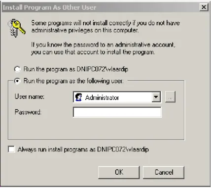
Figure 1. Intallation procedure – User screen.

You are asked to decide whether a person with administrator rights should install the program for you via the displayed dialog box. The choice for one of the options depends on your com-pany's protocols. It is advised to install the program using a user account with administrator rights. Click OK after having selected the correct user.

- In the following screen, click Next.

(19)

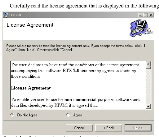
- Carefully read the license agreement that is displayed in the following dialog box:

Figure 3. Installation procedure – License Agreement screen.

- If you agree with the content of this agreement, select the I agree option, and then click Next.

Figure 4. Installation procedure – Select Folder screen.

- In the dialog box displayed above, select the Folder in which you want ETX to be

(20)

The default directory is C:\Program Files\RIVM\ETX 2.0. If you want to install ETX in an

other directory, click Browse and select the directory of your choice. - Click on Next to continue.

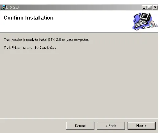
Figure 5. Installation procedure – Confirm Installation screen.

- In the dialog box displayed above, click Next if you want the installation to be carried out. - Installation will now be performed. If the .NET framework is not yet installed on your

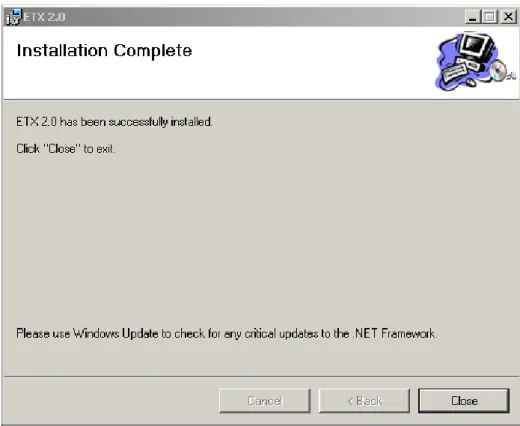
computer, it will be installed. Installation of this framework takes several minutes. - When the Installation is complete, the following screen appears. Click on Close to leave

(21)

Figure 6. Installation procedure –Installation Complete screen.

3.3 Removing E

_T

X

If you want to de-install (or remove) ETX, do the following.

- Under the Start button, click on Settings, Control Panel.

- In the Control Panel, double click the Add/Remove Programs icon.

- Select ETX from the list of currently installed programs. After clicking on ETX in this list,

you can select Remove.

- ETX will now be removed from you computer.

3.4 Starting E

_T

X

When ETX is installed successfully, the program can be found under the Start button in the

lower left corner of your screen. It will be placed under: Programs, RIVM ETX, E_TX 2.0.

Click on the ETX 2.0 icon to start the program.

3.5 Saving data in E

_T

X

If you save data in ETX, your data will be stored in a Project. This is a file with the

extension: etx. To save a Project, Click on File on the Menu bar, then click Save.

In order to set or change the default directory where your ETX projects will be stored, see

sections 5.1.5 and 5.9.4.

N.B. Your calculations and calculated results will not be stored together with your data. However, if you open an etx-Project that you had saved earlier, and press calculate again, all

(22)

results and output will be generated, together with the settings that were active at the time your Project was saved.

3.6 Starting a new project in E

_T

X

The ETX opening screen is always an empty project. You can start directly with entering data

here. Starting a new project can be performed by clicking on File, New in the Menu bar at the

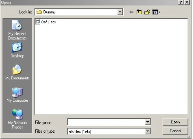
top of your ETX screen. Opening an existing project can be performed by clicking File, Open

input file. The following dialog box appears:

Figure 7. The dialog box shown after clicking Open input file.

Select the ETX project of you choice and click on Open. Your Project will now be retrieved

and opened.

3.7 _{Leaving ETX}

You can leave ETX 2.0 by choosing File, Exit from the Menu bar.

Figure 8. Dialog box shown upon leaving E_TX.

(23)

3.8 Changing the settings for the decimal character

The choice of the character used as decimal symbol or digit grouping symbol in numerical values within ETX is determined by the regional settings of your PC. In English or American

settings, the comma ',' is mostly used as digit grouping symbol, while the period '.' is used as decimal sign. In the Dutch language and settings, this is opposite, here the period '.' is used as digit grouping symbol and the comma ',' is the decimal sign. Please take notice that the re-gional settings will also apply to values printed along the axes of figures.

You may want to change these settings. Below, you find the route to the Control Box in which you can change your settings for several Microsoft operating systems.

3.8.1 Windows 98, NT, 2000 and ME

Click on the Start button in the lower left corner of your screen, then select Settings, Control Panel and Regional Settings (double click). In the Regional Settings properties box that has appeared, select the Number tab. In this screen you can either select a Region and obtain its accompanying settings or Customise your settings. After having made your selection, click on Apply and on OK. Changing of settings will have no effect unless you restart ETX.

3.8.2 Windows XP

Click on the Start button in the lower left corner of your screen, then select Settings, Control Panel, Regional and Language Options. Select the Regional Options tab. In this screen you can either select a Region and obtain its accompanying settings or Customise your settings. After having made your selection, click on Apply and on OK. Changing of settings will have no effect unless you restart ETX.

3.9 _{Comments on ETX}

If you have comments on the program, its functioning or other ideas, you can send these by e-mail to etx.info@rivm.nl. Please note that this is not a helpdesk address. We will not respond to questions, but we will collect comments, possible errors and ideas for future development. Unfortunately, we are unable to help all users with problems or questions.

(24)

(25)

4. Reference manual

In section 4.1 we outline the different sections in which the program can be divided. We also name all sheets and briefly explain their contents. Section 4.2 explains the meaning of each of the items you may encounter in ETX. A list of abbreviations is included at page 63 of this

re-port. How to use the information given in this chapter is explained to you in chapter 5 while chapter 7 tells you how to perform some calculations in practice.

4.1 Structure of the program

The program is divided in two major sections: an input and an output section. The input sec-tion has two subsecsec-tions: Input toxicity data and Input exposure data. Each will be briefly dis-cussed in the section 4.1.1. To get results, you have to invoke a calculation (section 5.7), which gives results in the Output section. The output section is divided in three sections,

which will be introduced in section 4.1.3.

4.1.1 Data input

We discern two types of data: toxicity data and environmental concentrations.

Figure 9. Subdivision of the input section.

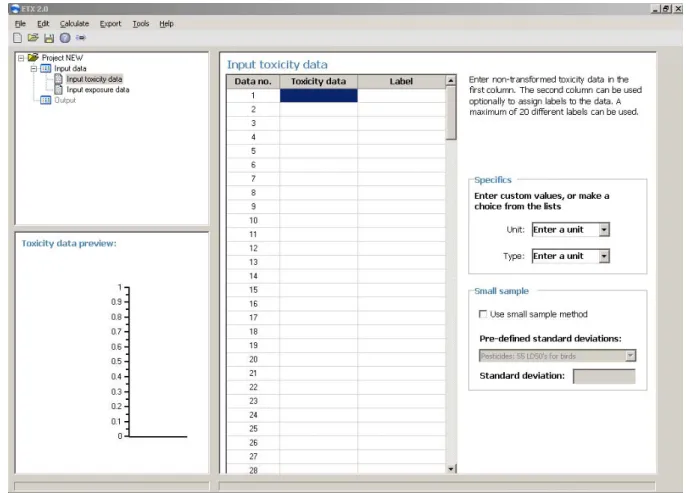
4.1.1.1 Input toxicity data

Figure 9 shows the two sections of Input data.

- If you want to calculate an SSD and the accompanying HC5 and HC50, you should enter your data in the Input toxicity data sheet. If you want to calculate an FA, you need an SSD

first. The output section will remain inaccessible until you have calculated an SSD. - For calculation of the HD5 for birds and mammals, there is room to enter a (small) data

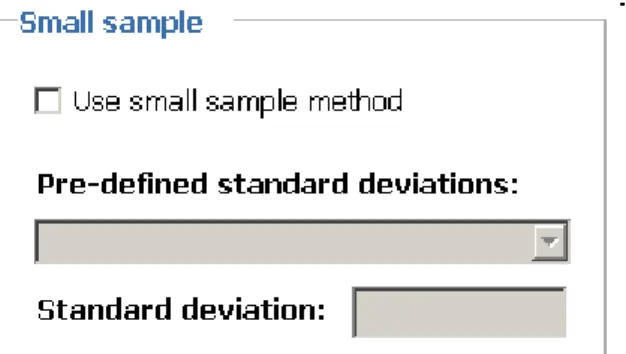
set of no more than 10 values. We call this the 'small sample' method. To use this method you have to select the check box labelled with Use small sample method in the lower right corner of the input screen (see Figure 10). You also have to enter a standard deviation

(26)

from an external data set. Entering data for the 'small sample' method is also done in the

Input toxicity data sheet.

Figure 10. Small sample box.

4.1.1.2 Input exposure data

After having entered data in the Input toxicity data sheet and after you have calculated the

ac-companying SSD, you can use the Input exposure data sheet to calculate either an FA or an EER. There is the possibility for input of a single exposure concentration and a separate input section in case you have a series of exposure concentrations (like a measurement series).

4.1.2 Types of calculations

You can perform four types of calculations. 1. Calculate an SSD only.

2. Calculate an SSD and an FA. An FA can only be calculated when you have entered data

in Input toxicity data and generated an SSD.

3. Calculate an SSD and an EER. An EER can only be calculated when you have entered data in Input toxicity data and generated an SSD.

4. Calculate a (small sample) HD5. A maximum of 10 data can be entered. Calculation of an SSD is not needed in this case.

All calculations are performed by clicking Calculate, Go on the Menu bar in each of the two

Input sections, or by clicking the Calculate button: . Please note that pressing the enter

key on your keyboard does not invoke a calculation.

After selecting the Calculate button (or using the menu), the calculation is performed and the

results will appear in one or more of the output worksheets or graphs (see section 4.1.3). NB. The program will also generate results and graphics if the outcome of the goodness-of-fit tests imply that it is less probable that your data derive from a normal distribution. The pro-gram only calculates, it does not make decisions. It is up to you to decide whether you accept or reject the presented outcome of the calculations.

4.1.3 Output

4.1.3.1 SSD related output

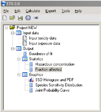
The Output section contains three subsections and each of the subsections contains one or

more sheets. Figure 11 shows the available output sheets in the program tree below Output. The contents of each sheet are outlined below.

(27)

Figure 11. Subdivision of the output section for SSD calculations.

4.1.3.1.1 Goodness-of-fit

This sheet shows you the results of three goodness-of-fit (GOF) tests performed on your toxicity data. A brief explanation on the interpretation of these tests is also given. If you have entered a series of environmental concentrations in the Input exposure data sheet and have

invoked a calculation, you will find the GOF test on these data here.

4.1.3.1.2 Statistics

In this section, two sheets can be found, the content of each is described below.

Hazardous concentration

In this sheet the mean and standard deviation (s.d.) of the normal distribution through your data are reported as well as the sample size. Furthermore, the HC5, FA at the HC5, the HC50 and the FA at the HC50 are reported. For each of these parameters, the lower and upper limit of the 90% confidence interval around the median estimate are reported.

Fraction affected

The estimated FA (plus lower and upper estimate of the two-sided 90% confidence interval) at the exposure concentration (EC) that you have entered in the Input exposure data sheet in

the single PEC input cell is reported in this sheet. If you have entered a series of exposure

concentrations in the Input exposure data sheet, the EER is reported.

4.1.3.1.3 Graphics

There are 3 sheets that show graphical output.

SSD Histogram and PDF

A histogram (or frequency distribution) of your toxicity distribution is presented when you have calculated an SSD. The bin width (classwidth) is calculated according to the method of Scott (1992) as:

(28)

3 / 1 5 . 3 n eviation standard d binWidth = ×

The placement of bins on the x-axis is described in more detail in section 4.2.5. The height of the bars is expressed as the number of data they represent, which is plotted on the right hand

y-axis. The normal distribution plotted in this graph is the probability density function (PDF)

that is associated with your toxicity data sample. The left hand y-axis shows the density of the toxicity data. The left hand y-axis can also be used to read the densities of the bars in the his-togram. For both the PDF and the histogram, the integral of all data, i.e. the sum of class-width ´ density, equals 1.

Species sensitivity distribution

If you have calculated an SSD, this is the cumulative density function (CDF) that is associ-ated with your toxicity data sample. The dots in the graph are placed at the so-called Hazen plotting positions: pi = (i – 0.5)/n (see Aldenberg et al., 2002).

Joint probability curve

This graph shows the joint probability curve (JPC). To obtain a JPC you have to enter toxic-ity data in the Input toxicity data sheet and a series (n>1) of exposure concentrations in the

Input exposure data sheet. After having calculated an SSD, the JPC will be generated.

4.1.3.2 Small sample output

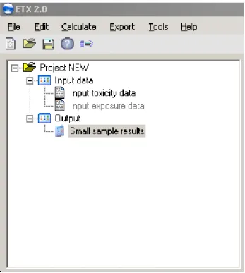
When the 'small sample' method is used, no SSD is required. The Output section only shows

the Small sample results sheet (Figure 12). The content of the output sheet is outlined below.

Figure 12. Subdivision of the output section for small sample calculations.

4.1.3.2.1 Small sample results

The median estimate of the HD5 of your small data set is calculated and presented together with its 90% confidence interval limits. Also presented are the extrapolation factors that can be used to directly calculate the lower limit (LL), median or upper limit (UL) estimate of the HD5 from the sample mean.

(29)

4.2 Glossary of keywords

In this section, a description of keywords is given, listed in alphabetical order. Keywords are those items you may encounter on the input or output screens of ETX. This section gives a

brief explanation of each keyword, but we do not go deeply into the theoretical background of each item in this manual. For more background information, we refer to the underlying literature, which is listed in the Reference section of this manual.

4.2.1 Exposure concentration (EC)

In this manual and in ETX 2.0, the parameter 'exposure concentration' is synonym with

'envi-ronmental concentration'. Both can be abbreviated as EC and both are interchangeable in manual and program.

4.2.2 Expected Ecological Risk (EER)

An EER can be calculated if a set of predicted exposure concentrations (ECs) is entered in the input section of the program. Mean and s.d. are scaled relative to the mean and s.d. of the species sensitivity distribution. The EER literally is the probability that a randomly drawn species for a random draw of exposure is affected.

The following statistical parameters will appear in the Fraction affected output screen (in or-der of appearance):

SECmean, SECsd and EER

SEC stands for scaled environmental concentration.

- The SECmean is the scaled mean of the environmental concentration distribution. It is re-ported here as the log10 transformed value.

- SECsd is the scaled s.d. of the environmental concentration distribution. It is reported here as the log10 transformed value.

- EER is the expected (mean) ecological risk, given the SSD and the distribution of envi-ronmental concentrations. The EER is the area below the curve in the joint probability curve (Output, Graphics).

4.2.3 Extrapolation factor

In the Small Sample Output sheet, extrapolation factors are displayed. These can be found in

the HD5 (median) results box on your screen.

Extrapolation factors are factors to be applied multiplicatively to the geometric mean of the original (not log-transformed) toxicity data. Extrapolation factors depend on the FA, sample size, confidence level and on the standard deviation of the SSD (Aldenberg and Luttik, 2002). In ETX 2.0, extrapolation factors are given for an FA of 5% (HD5) for the upper and lower

limit of the 90% confidence interval of the HD5.

4.2.4 Fraction affected (FA)

An FA can be calculated when one single predicted exposure concentration (EC, synonym with PEC) value is available. This EC value can be entered in the input section of the pro-gram. The following statistical parameters will appear in the Output screen. In order of ap-pearance:

LL FA, Median FA and UL FA

Reported is the median estimate of the FA at the PEC you have entered. Also reported is the two-sided 90% confidence interval of the FA: LL FA represents the 5% confidence limit and

(30)

UL FA represents the 95% confidence limit. These calculations are based on repeated linear interpolation and are approximate values. The procedure is explained in section 8.2.3 of Al-denberg and Jaworska (2000). A precise answer can be obtained using the functions de-scribed in section 8.2.1 of that paper.

This routine does not yield results when your standardised mean logarithmic effect concen-tration is <-5 or >5. As a check, the value of the standardised logarithmic concenconcen-tration cal-culated from your PEC value is shown in the Fraction affected output sheet. If this value is

outside the range mentioned above, no results will be given. The message

'The method does not yield results because your standardised PEC exceeds the limits of <-5 or >5' will appear in red. The sheet will show 'Out of bounds!' as error values.

4.2.5 SSD Histogram and PDF

This graph is a histogram or frequency distribution in which the toxicity data are represented by bars. On the x-axis the log10 of toxicity values (NOEC, LC50s etc.) is plotted. On the right hand y-axis, the frequency of the toxicity values is plotted. Toxicity values are distributed over frequency classes (often referred to as bins) that have a width calculated according to Scott (1992): 3 / 1 5 . 3 n eviation standard d binWidth = ×

The placing of bins on the x-axis is worked out as follows:

1. The number of bins is calculated using the equation mentioned above;

2. Bins are divided over the range of toxicity data by centering around the mean (=sample mean, or mean of the toxicity data);

3. Sample values coinciding with a bin limit are dropped in the next lower bin.

4. In case the lowest sample value coincides with the lower limit of the lowest bin, this value is dropped in this lower bin.

In case of an even number of bins, we identify two middle bins. The mean of the toxicity data now coincides with the separation between the two middle bins. More precise, the mean value itself is chosen to coincide with the highest value of the left bin (due to point 3 above). In case of an uneven number of bins, there is one middle bin. In these cases, the middle of the middle bin is chosen to coincide with the mean of the toxicity data.

4.2.6 Goodness-of-fit

Whether the sample of toxicity data derives from a normal distribution can be assessed with goodness-of-fit tests. Two different types of tests are implemented, based on quadratic (verti-cal) distance and on the largest vertical distance. Well-known quadratic tests are the Ander-son Darling test and the Cramér-von Mises test (cf. D'Agostino and Stephens, 1986). The Kolmogorov-Smirnov test is a well-known vertical distance test (D'Agostino and Stephens, 1986).

1. The Anderson-Darling goodness-of-fit test highlights differences between the tail of the distribution and the input data and is generally regarded as a very powerful general test (Aldenberg et al., 2002).

2. The Kolmogorov-Smirnov test focuses on differences in the middle of the distribution and is not very sensitive to discrepancies of fit in the tail of the distribution.

Interpreting Critical Values

If a test statistic is above the 5% critical value, normality is rejected at the 5% critical value, indicating doubts about normality.

(31)

If a test statistic is below the 5% critical value, normality is accepted (not rejected) at the 5% critical value.

If a higher critical value is accepted (e.g. at 2.5% significance level), then the probability that these data derive from a normal distribution is smaller than at 5%, but it is not impossible that the sample derives from a normal distribution.

Some people find it confusing that a higher significance level, say 10%, has a lower critical value. 'Rejected' occurs more often with a higher significance level. In conclusion: a GOF test does NOT say that a sample cannot derive from a normal distribution, just that it becomes less probable with decreasing significance levels.

4.2.7 HC

5

and HC

50

Your toxicity dataset refers to a selection of species, which is treated as a sample drawn from a population (in a statistical sense). By definition, the calculated normal distribution encom-passes all species inhabiting the environmental compartment of interest. It is up to you to de-termine whether your sample of species is representative for the population of species (in a biological sense) you want to derive HC values for. The distribution is the –estimated– func-tion that relates the relative sensitivity of the species thought present in a given environmental compartment to (the logarithm of) the toxicant concentration. This distribution is a normal distribution (by definition) when you use ETX 2.0 for your calculations. HC is short for

'haz-ardous concentration'. HC5 and HC50 are the 5th and 50th percentile (median is synonymous for the latter) of the normal distribution that is fitted through the toxicity data you have en-tered. HC5 and HC50 are expressed as a toxicant concentration (in the same units as the toxic-ity data you have entered in the input section). Hence, they represent the toxicant concentra-tion that is hazardous to 5 or 50 percent of 'all' species. See secconcentra-tion 4.2.11 for explanaconcentra-tion of the HC parameters calculated by ETX 2.0.

4.2.8 JPC

The abbreviation stands for joint probability curve. This is a graphical representation of the risk of a substance to the species, that may be used in risk characterisation. The type of graph

ETX shows is a cumulative profile plot. It is constructed by plotting FA values from the SSD

(in CDF form) on the y- axis against exposure concentration distribution (ECD) values (also in CDF form) on the x-axis at corresponding log-exposure concentrations. The area under the curve (AUC) is equal to the expected ecological risk. For more detail, see Aldenberg et al. (2002). The numerical value of the AUC, or EER, is shown in the Fraction affected sheet

(Output, Statistics).

4.2.9 PEC

If an environmental concentration of the substance of interest is the outcome of some model calculation rather than a measured value –or series of values– in the field, it is called a

pre-dicted environmental concentration. If you have a single PEC value and an SSD, you can

cal-culate the fraction of species described by that SSD that is (potentially) affected by the sub-stance.

4.2.10 Small Sample method

The idea to estimate a percentile of an SSD and its uncertainty for a very small sample of toxicity data has emerged from the field of pesticide registration. Due to the limited size of the sample, there is no reliable information on the standard deviation of the SSD. A standard deviation from a different sample, to which one attaches more confidence because it has higher reliability, is used to estimate the HD5. Luttik and Aldenberg (1997) published this method for logistically distributed toxicity data.

(32)

The method that is currently implemented in ETX 2.0 offers the possibility to calculate HD5 values for birds or mammals based on normally distributed toxicity data (Aldenberg and Lut-tik, 2002). From a dataset of 55 pesticide LD50 values for birds a pooled variance estimate of the standard deviations of all LD50 values was calculated. The same was done for a dataset of 69 pesticide LD50 values for mammals. From both datasets the pooled variance estimates for carbamates and organophosphorous compounds were also calculated. All pooled variance estimates are listed in the Input toxicity data sheet in the Small sample box (under Pre-defined

standard deviations). These estimates can be used as an ('external') standard deviation that is

assumed to describe the spread of the population from which your (small) sample of bird/mammal data has been drawn.

Recommendations to the 'small sample' method:

(i) When there are indications that the (small) sample standard deviation does not reflect the population standard deviation, even when n ≥ 4, consider using the pooled standard deviation (i.e. use the 'small sample' technique). A maximum of 10 entries is allowed for in the Input toxicity data sheet.

(ii) Use the LL HD5 values or corresponding assessment factors when a 5% probability for overestimation of the HD5 is desired. When the median HD5 or its corresponding assessment factor is used, 50% probability for HD5 overestimation is allowed.

(iii) When there are indications that the available data are derived from a test with a sensitive species, one could consider using the median estimate of the HD5 or the corresponding ex-trapolation factor.

4.2.11 Statistics SSD

If an SSD has been calculated by ETX, i.e. if a normal distribution has been fitted through

your toxicity data, the following statistical parameters will appear in the Hazardous

concen-tration output screen (in order of appearance).

Mean, s.d. and n

Mean and s.d. are the sample mean and the sample standard deviation (n-1) of the normal distribution. These parameters are shown in log10 units and are the parameters that describe the normal distribution fitted through your toxicity data set. n is the sample size, i.e the num-ber of toxicity data. It is shown because the size of n directly determines the size of the un-certainty in the HC5 and HC50 (Aldenberg and Jaworska, 2000). These sample statistics are used to estimate the SSD parameters.

HC5 results: LL HC5, HC5, UL HC5 and sprHC5

These parameters are shown in the same concentration units as you entered your toxicity data in. Presented are the estimated 5th percentile of the normal distribution (HC5) and its two-sided 90% confidence limits, called the lower limit (LL) and upper limit (UL), respectively. The HC5 itself is a normally distributed statistic, and sprHC5 is a measure of the width of the HC5 distribution. It is calculated as the ratio of UL and LL.

FA at HC5 results: FAlower, FAmedian and FAupper

The median estimate of the FA at the toxicant concentration HC5, is 5%, by definition, since the HC5 is the 5th percentile of the SSD. The two-sided 90% confidence interval for the FA is also reported: FAlower represents the 5% confidence limit of the FA and FAupper represents the 95% confidence limit.

(33)

These parameters are shown in the same concentration units as you entered your toxicity data in. Presented are the estimated median or 50th percentile of the normal distribution (HC50) and its two-sided 90% confidence limits, called the lower limit (LL) and upper limit (UL),

respectively. The HC50 itself is a normally distributed statistic, and sprHC50 is a measure of the width of the HC50 distribution. It is calculated as the ratio of UL and LL.

FA at HC50 results: FAlower, FAmedian and FAupper

The median estimate of the FA at the toxicant concentration HC50, is 50%, by definition, since the HC50 is the 50th percentile of the SSD. The two-sided 90% confidence interval for the FA is also reported: FAlower represents the 5% confidence limit of the FA and FAupper re-presents the 95% confidence limit.

4.2.12 SSD

ETX calculates an SSD from your sample of toxicity data assuming that the (continuous)

tribution describing the sensitivity of the population underlying your sample is normally dis-tributed over log concentration. This Gaussian distribution is graphically presented in the

SSD Histogram and PDF sheet (to be found under Output, Graphics). The data and the fitted

distribution are also presented as a CDF plot in the SSD sheet (Output, Graphics). The

statis-tical parameters derived from this distribution are presented in the Hazardous concentration

(34)

(35)

5. Working with E

_T

X

5.1 Menu bar and buttons

The menu bar and buttons that are available in ETX are shown in Figure 13. Throughout the

program, the same menu bar and buttons will appear. All functions that may be accessed via the menu bar will not be described here individually, we will give a general description of each menu item. Most items you will encounter when you work through the manual or by just trying them!

Figure 13. Menu bar and buttons in ETX.

5.1.1 File

Options provided here allow you to: - start a new ETX project (New).

- open an existing ETX project (Open input file). When you have saved your work in an ETX

project, ETX does not save the calculated data and graphs. If you want to see the results

again, simply press Calculate after opening an existing ETX project and your results will

reappear. If you want to save all data, choose Export and all your results will be placed in an Excel spreadsheet.

- save your work (Save).

- save your project under a different name (Save as). - leave ETX (Exit).

5.1.2 Edit

The options provided here allow you to handle individual cells or ranges of cells, that you can either delete, cut, copy and paste.

5.1.3 Calculate

The only option provided here is to invoke a calculation. The function of this menu is equal to that of the calculate button (section 5.1.7). For more information on the types of calcula-tions you can perform, see section 5.7.

5.1.4 Export

The only option provided here is to export the data you have entered and calculated, to a separate file. The data will be exported in Microsoft Excel spreadsheet format. See also sec-tion 5.8. To change the default directory where projects and exported files are stored, see section 5.9.

5.1.5 Tools

There are four options here: Labels, Sort toxicity data, Sort labels and Preferences.

- Use Labels to attach label to the entries in the toxicity data sheet. For more information

please see section 5.6.

- By clicking on Sort toxicity data, the toxicity data in the Input toxicity sheet will be sorted

(36)

- By clicking on Sort labels, the labels in the Input toxicity sheet will be sorted in alphabeti-cal order. NB: this operation can not be undone.

- Use Preferences to define the default settings for the looks of your graphs and to set the

default directory where projects and exported files are stored. For more information please see section 5.9.

5.1.6 Help

In the Help menu, there are two options to choose: E_TX Help topics and About ETX 2.0. When you select the help topics, you can use the E_TX 2.0 manual online. The content of this menu is

equal to the content of this manual.

About ETX 2.0 gives you information on the version of this program. Information on earlier

versions of ETX is also provided.

5.1.7 Buttons

The buttons have the following names and function: New. This button opens a New ETX project.

Open existing project.

Save. Allows you to save the current project. Help. Allows you to access the Help file. Calculate. Invokes a calculation.

5.2 Navigating through E

_T

X

(37)

Figure 14. ETX appearance after starting the program.

This screen is divided in three major parts: in the upper left corner: the navigating section, in the lower left corner: the Toxicity data preview section and the largest part is the right half of the screen: the Input toxicity data section. In the navigating screen, you find + or – signs. By

clicking on these you can unfold or fold a specific part of the program and view or hide its contents. Use these buttons to find out that each ETX project contains an Input data section

and an Output section. If you select a specific section or sheet by clicking on it, it will be dis-played in the right half of your screen. In the following, you will be guided through each of the different parts of the program.

5.3 Entering data

5.3.1 Toxicity data

- Go to the Input toxicity data sheet in the Input data section of ETX.

- Go to the Input toxicity data box (this is the right part of your screen).

- Next, in the cells under Toxicity data, enter your toxicity values as a column, with one value per input cell. Enter the toxicity data in the original (non-transformed) values. - For information on entering the unit of your data or the type of endpoint, see

section 5.3.2.

- For information on labelling of your toxicity data, see section 5.6. - Make sure all entries have the same unit: mg/l, µg/kg, ppm etc.

- You cannot enter the value 0 (zero). Your data will be log10-transformed for calculation and log(0) does not exist. If you enter a zero value, the error message Please enter only

(38)

positive values will be displayed at the bottom of your screen. Delete the zero value or

enter a positive non-zero value to continue. - You need not sort the data.

- You may leave blank cells, empty cells will not be included in the graph or in calcula-tions.

- For HC5 and HC50 calculation a maximum number of 200 data can be entered.

- For FA and FA-confidence limits the maximum number of data (n) =75 for FA at HC50 and n = 200 for FA at HC5.

When you have finished entering data, see section 5.7.1 on how to calculate an SSD.

5.3.2 Assigning units to your data

You may enter the unit of toxicity data and/or exposure data. It is optional to do this, but there are two reasons to do so. First, if you are about to enter both toxicity and exposure data e.g. to calculate a fraction affected, the data should be entered in ETX in the same units!

Second, if you enter the unit of your data, this unit will be printed in the output of your data that is exported to Excel.

To assign a unit to your data go to the Input toxicity data section. In the lower right half of

your screen, you find the Specifics box (Figure 15):

Figure 15. The specifics box.

- In the scrollbar to the right of Unit, you may type a unit of your choice or select the unit from the pulldown menu.

- In the scrollbar to the right of Type, you may type the endpoint of the toxicity data you are about to enter, or you can select an endpoint from the pulldown menu.

- The Specifics box functions as a piece of scrap paper. Both options in the box remind you

that all toxicity data should be of the same unit and type. Unit and type are not linked to any calculation. They reappear in the Input exposure data section, to remind you that the

units of data entered in that section should be identical to the units of the data entered in the Input toxicity data section.

- Use of the Specifics box is optional. ETX works equally well when you clear the contents

of the Unit and Type boxes.

5.3.3 Small sample data

- Go to the Input toxicity data sheet in the Input data section of ETX.

- In the Input toxicity data box (this is the right part of your screen), click on the Use small

sample approach check box in the Small sample box. The following dialog box will

(39)

Figure 16. Small sample verification box.

If you had already typed data in the input section, these data will be lost when you switch to the Small sample input mode. Remember that this is a different method that does not require calculation of an SSD. So, if you want to keep the data you had entered before, click on Can-cel and Save your work in an ETX project. Then start a new project for your 'small sample'

calculation. Otherwise, click on OK.

- The number of toxicity data that you can enter is now limited to 10.

- Enter your toxicity values as a column, with one value per input cell. Enter the toxicity data in the original (non-log transformed) format.

- Make sure all entries have the unit of mg/kg body weight.

- You cannot enter the value 0 (zero). Your data will be log10-transformed for calculation and log(0) does not exist.

- You need not sort the data.

- You may leave blank cells, empty cells will not be included in calculations.

- Enter a standard deviation. In the Small sample box at the lower right corner of your input

screen, you can choose one of several pre-defined pooled standard deviations. The ac-companying value that will be used for calculations appears in the Standard deviation

box.

When you have finished entering data, see section 5.7.2 on how to calculate an HD5.

5.3.4 Environmental concentrations

5.3.4.1 One environmental concentration

This calculation applies when you have only one environmental concentration, e.g. a PEC resulting from the exposure part of a risk assessment rather than a series of measurements. - Go to the Input exposure data sheet in the Input data part of ETX.

- You need to have an SSD before you can enter exposure data. Refer to section 5.3.1 for information on this subject. If you enter exposure data without having an SSD, the fol-lowing message will pop up:

Figure 17. Message displayed upon FA calculation when no toxicity data have been entered.

- Enter your PEC value in the Single PEC box at the right part of your screen.

- Make sure that the unit of your PEC value is identical to the unit of the toxicity values that you have entered to generate your SSD! The unit of your toxicity data will be dis-played in the Specifics box when you have made use of it while entering of your toxicity data.

(40)

- Enter a non-log transformed PEC value!

- This routine does not yield results when your standardised logarithmic PEC is <-5 or >5. The value of the standardised logarithmic concentration PEC will be shown in the Frac-tion affected sheet (Output, Statistics).

When you have finished entering data, see section 5.7.3 on how to calculate an FA.

5.3.4.2 A series of environmental concentrations

This calculation applies when you have a series of environmental concentrations, e.g. a measurement series of the compound of interest in an environmental compartment. - Go to the Input exposure data sheet in the Input data part of ETX.

- Go to the Input environmental concentrations box (this is the right part of your screen). - In the cells under Exposure data, enter your toxicity values as a column, with one value

per input cell.

- Enter the toxicity data in the original (non-transformed) values.

- Make sure that the unit of your environmental concentrations is identical to the unit of the toxicity values that you have entered to generate your SSD! The unit of your toxicity data will be displayed in the Specifics box when you have made use of it during entering of your toxicity data.

- Make sure all entries have the same unit: mg/l, µg/kg, ppm etc.

- You need not sort the data.

- You may leave blank cells, empty cells will not be included in the graph or in calcula-tions.

When you have finished entering data, see section 5.7.4 on how to calculate an EER and JPC.

5.4 Clearing the contents of the input cells

5.4.1 Clearing a single cell

You can clear (or delete) data in a single input cell as follows. - Select the cell you want to by clicking in the cell.

- Click on Edit, Delete in the Standard menu bar or press the Delete button on your

key-board to clear the content of the selected cell. The following message will appear:

Figure 18. Message displayed when cell contents are about to be deleted.

(41)

5.4.2 Clearing all cells

In order to clear a range of cells, do the following:

- Select the uppermost cell of the range of cells you want to clear, by clicking in the cell. - Press the Shift button together with the Arrow Down (↓) button (both on your keyboard).

While holding the shift button pressed down, you can select multiple cells by using the ↓ button repeatedly.

- When you have reached the bottom cell of the range you want to clear, stop holding down keys. Your selection of cells is now highlighted.

- Click on Edit, Delete in the Standard menu bar or press the Delete button on your key-board to clear the content of the selected cells.

In order to clear all cells, do the following: - Select the upper cell by clicking in it.

- Press the Shift button together with the Ctrl button. While holding these buttons pressed down, click on the Arrow Down (↓) button (all buttons are on your keyboard).

- All cells will now be selected (highlighted).

- Click on Edit, Delete in the Standard menu bar or press the Delete button on your

key-board to clear the content of the selected cells.

5.5 Importing data

You can also enter data (both toxicity data and environmental concentrations) from e.g. MS Excel. The procedure is as follows:

- The data you want to import should be placed in a column. - Select the column containing your data and copy it

- Switch to ETX and click once in the upper cell of the data column of the sheet in which

you want to import your data. - Paste the data.

Please refer to section 5.11 on how to use the decimal symbol in these type of operations.

5.6 Adding labels to toxicity data

NB. This function is optional. All other program functions can be executed equally well when the toxicity data are not labelled.

When entering toxicity data, you have the possibility to label your entries. This means that you can add a text label to toxicity data. You might, for example, want to discriminate be-tween the different taxonomic levels in your SSD and add labels like algae, crustacea,

in-secta (or abbreviations). Apart from adding text labels, you can customise the appearance of

the symbols that are linked to your labels. These symbols will be used to construct your SSD.

5.6.1 Creating a label collection and using labels

Before you can enter labels that will also appear in your SSD graph, you have to create a la-bel collection. To create a lala-bel collection, do as follows:

- Click on Tools, Labels in the Menu bar and the Input toxicity data labels dialog box shown in Figure 19 will appear:

(42)

Figure 19. The Input toxicity data labels box.

- Next, type the name of the label in the column Label and assign a Color and a Symbol to the label in the following columns. Complete your label collection in this way.

- After having completed your label collection, click the Save button in the top part of the

Input toxicity data labels box and type the name of your label collection. The name will

now appear in the Stored label collections box visible at the top of the dialog box. - You can select a label collection by clicking on its name in the Stored label collections

box and subsequently press the Select button at the bottom of the label box. You then

automatically return to the Input toxicity data sheet.

- Back in the Input toxicity data screen you see the selected label collection displayed in the

lower right corner of your screen:

Figure 20. The active label collection display.

- Back in the Input toxicity data screen, behind each of the toxicity data that you enter, there is a Label cell. Using the pull down menu in each cell, you can now choose one of the

(43)

taxonomic groups (or 'labels') that are present in the label collection you have just se-lected.

5.6.2 Editing an existing label collection

Editing an existing label collection can also be performed via the Input toxicity data labels

dialog box:

- Click on Tools, Labels in the menu bar and the Input toxicity data labels dialog box shown in Figure 19 will appear.

- Select the label collection in the Stored label collections box by clicking on it.

- Edit the label collection.

- Press the Save button to save any changes.

- Press the Select button if you wish to select the current label collection. You will

auto-matically leave this dialog box after clicking Select.

5.6.3 Deselecting a label collection

In case you want to clear the connection between the toxicity data you have entered and the selected label collection, do the following:

- In the Input toxicity data screen you see the Label collection display in the lower right

cor-ner of your screen (Figure 20).

- Click on the Deactivate button to clear all labels entries behind your toxicity data.

- Note that this action will not erase your label collection or its settings, only its connection with the current dataset.

5.7 Performing calculations

5.7.1 Calculating an SSD

When you have finished entering toxicity data in the Input toxicity data sheet, you are ready to calculate an SSD.

- Select Calculate, Go from the Standard menu bar or press the Calculate button: to in-voke the calculation of the SSD and its statistics.

- After performing the calculation, ETX will automatically switch to the Hazardous

concen-tration sheet in the Output, Statistics section.

- Switch manually to the Goodness-of-fit section in order to check the result of the

norma-lity tests performed on your toxicity data.

- Two graphs will be generated as well: the histogram and an SSD. Both can be found un-der Output, Graphics.

- If you have deleted or added data in the input section, choose Calculate, Go from the Standard menu bar (or press ) again for an update of statistics and graphics.

5.7.2 Calculating a small sample HD

5

When you have finished entering toxicity data in the Input toxicity data sheet using the 'small

sample' method, you are ready to calculate an HD5.

- Select Calculate, Go from the Standard menu bar or press the Calculate button: to

in-voke the calculation of the HD5 and its statistics.

- After performing the calculation, ETX will automatically switch to the Small sample

(44)

- If you have deleted or added data in the input section, choose Calculate, Go from the Standard menu bar (or press ) again for an update of statistics.

5.7.3 Calculating an FA

When you have calculated an SSD and finished entering exposure data in the Input exposure data sheet, you are ready to calculate an FA.

in-voke the calculation of the FA and its statistics.

- After performing the calculation, ETX will automatically switch to the Fraction affected

sheet in the Output, Statistics section.

- If you have deleted or changed your PEC in the input section, choose Calculate, Go from the Standard menu bar (or press ) again for an update of statistics.

5.7.4 Calculating an EER and JPC

When you have finished entering a series of environmental concentrations in the Input

expo-sure data sheet, you are ready to calculate an EER and JPC.

in-voke the calculation of the EER and its JPC.

- After performing the calculation, ETX will automatically switch to the Fraction affected

sheet in the Output, Statistics section. This sheet shows the EER in the lower one of the

two boxes.

- Switch manually to the Goodness-of-fit section in order to check the result of the norma-lity test performed on your exposure data.

- A joint probability curve will be generated as well. It can be found under Output,

Graphics.

- If you have deleted or added data in the input section, choose Calculate, Go from the Standard menu bar (or press ) again for an update of statistics and the JPC.

5.8 Exporting results

Once you have generated results and statistics, you might want to save these results or store them in some other format. This can be done by using the Export function. You can find the

Export function in the menu bar. Clicking on Export shows you one menu option: Export

cur-rent output. After selecting this option, your data, statistical output en graphs will be exported

to an MS Excel spreadsheet (extension .xls). The default filename is identical to the name of your ETX project. If you have not yet stored you data in an ETX project, the default filename

(45)

Figure 21. Save export file dialog box.

After having selected the location of your choice, click on Save. You will be asked if you want to open the export file directly or not:

Figure 22. Export completed dialog box.

In order to have the exported (Excel)filenames corresponding with your ETX-project names,

save your ETX data in an ETX-project before exporting data to an Excel sheet. The name of

your ETX-project will then be chosen as default filename for your exported data file.

5.9 Preferences

5.9.1 Changing graph appearance in the current project

The three graphs that may be generated with ETX 2.0 can be edited to a limited extent. This

section explains how.

- Go to one of the graphs that you have generated: SSD Histogram and PDF, Species sensi-tivity distribution or Joint probability curve under Graphics.

- In the graph of your choice, click with the right mouse button (left button for left handed mousers).

- A pop up-window appears in which you can select various parts of the graph that you might want to edit (e.g. Title, Title font, labels, line colour etc.).

(46)

- All changes that you have made using this option will be saved along with your project. When you re-open a project and press calculate, the settings you last made will appear in your graphs.

5.9.2 Changing the axis settings

There are three possible graphs in ETX: an SSD Histogram and PDF, a Species sensitivity

dis-tribution and a Joint probability curve. The axis settings of the SSD Histogram and PDF can

not be changed. Axis settings for the other two graphs can be changed as follows:

- Go to one of the graphs that you have generated: SSD Histogram and PDF, Species sensi-tivity distribution or Joint probability curve under Graphics.

- In the graph of your choice, click with the right mouse button (left button for left handed mousers).

- A pop up-window appears in which you can select various parts of the graph that you might want to edit (e.g. Title, Title font, labels, line colour etc.). Select Axes settings

from the appearing menu. The following dialog box appears:

Figure 23. Axes settings dialog box.

ETX 2.0. A Program to Calculate Hazardous Concentrations and Fraction Affected, Based on Normally Distributed Toxicity Data

ETX 2.0

Rapport in het kort

Abstract

Contents

Samenvatting

Summary

1.

Introduction

1.1

Referring to E

X 2.0

2.

What can E

T

X 2.0 do for me?

3.

User's guide

3.1

Program type and system requirements

3.2

Installing E

X 2.0

3.3

Removing E

T

X

3.4

Starting E

T

X

3.5

Saving data in E

T

X

3.6

Starting a new project in E

T

X

3.7

Leaving ETX

3.8

Changing the settings for the decimal character

3.8.1 Windows 98, NT, 2000 and ME

3.8.2 Windows XP

3.9

Comments on ETX

4.

Reference manual

4.1

Structure of the program

4.1.1 Data input

4.1.2 Types of calculations

4.1.3 Output

4.2

Glossary of keywords

4.2.1 Exposure concentration (EC)

4.2.2 Expected Ecological Risk (EER)

4.2.3 Extrapolation factor

4.2.4 Fraction affected (FA)

4.2.5 SSD Histogram and PDF

4.2.6 Goodness-of-fit

4.2.7 HC

and HC

4.2.8 JPC

4.2.9 PEC

4.2.10 Small Sample method

4.2.11 Statistics SSD

4.2.12 SSD

5.

Working with E

T

X

5.1

Menu bar and buttons

5.1.1 File

5.1.2 Edit

5.1.3 Calculate

5.1.4 Export

5.1.5 Tools

_T

_T

_T

_T

_T

_{Leaving ETX}

_{Comments on ETX}

_T

_T