The practicability of the integrated probabilistic risk assessment (IPRA) approach for substances in food

(1)

The practicability of the integrated

probabilistic risk assessment approach

for substances in food

Report 320121001/2009 B.G.H. Bokkers et al.

(2)

RIVM report 320121001/2009

The practicability of the integrated probabilistic risk

assessment (IPRA) approach for substances in food

B.G.H. Bokkers M.I. Bakker P.E. Boon (1) P. Bos S. Bosgra

G.W.A.M. van der Heijden (2) G. Janer

W. Slob

H. van der Voet (2)

(1) RIKILT-Institute of Food Safety, Wageningen University and Research Centre (2) Biometris, Wageningen University and Research Centre

Contact: B.G.H. Bokkers

Centre for Substances and Integrated Risk Assessment bas.bokkers@rivm.nl

This investigation has been performed by order and for the account of the Food and Consumer Product

(3)

Parts of this publication may be reproduced, provided acknowledgement is given to the 'National Institute for Public Health and the Environment', along with the title and year of publication.

(4)

Abstract

The practicability of the integrated probabilistic risk assessment (IPRA) approach for substances in food

In the Netherlands, the National Institute for Public Health and the Environment (RIVM) has successfully applied the IPRA approach to assess the human health risks of five substances in food. This method has been developed so that health risks can be described in more detail when a classical risk assessment has shown either that there is a risk or a risk cannot be excluded. Using the IPRA approach enables more information to be gained on the fraction of the affected population in relation to the severity of the effect. Based on this information, authorities can then take targeted measures to prevent any risk to human health. It is expected that the IPRA methodology will be suitable for use with other substances.

The above has been concluded from research performed by the RIVM in collaboration with Biometris and RIKILT – organizations that fall under Wageningen University and Research Centre. The research was commissioned by the Dutch Food and Consumer Product Safety Authority (VWA)

In the present study, the risks of two mycotoxins (DON and T-2/HT-2), one heavy metal (cadmium), one group of pesticides (OPs), and one compound (acrylamide) which is formed during the heating of food containing high levels of starch are described. The IPRA approach enables the amount of a substance with which a population is exposed to that substance through food to be compared with the maximum safe level. Differences between individuals and possible calculation errors have been accounted for. The IPRA showed that the exposure of the five substances studied was below the levels considered safe. The health risks can therefore be considered negligible.

Furthermore, the method can provide more insight on which additional information could be gathered in order to improve the risk assessment. This would help targeted follow-up research to take place.

Key words: probabilistic risk assessment, exposure, toxicological effect, extrapolation factor, benchmark dose

(5)

(6)

Rapport in het kort

De bruikbaarheid van een geïntegreerde probabilistische (IPRA) methodiek voor de risicobeoordeling van stoffen in voeding.

Het RIVM heeft de IPRA-methode succesvol toegepast om de gezondheidsrisico’s voor de mens van vijf stoffen in voeding te beschrijven. Deze methode is ontwikkeld om de risico’s gedetailleerd te kunnen beschrijven als uit klassieke risicobeoordelingen blijkt dat er risico’s zijn, of als risico’s voor de gezondheid niet uitgesloten kunnen worden. Met de IPRA-methode is het mogelijk om aan te geven welk deel van de bevolking risico loopt nadat zij aan stoffen is blootgesteld en hoe ernstig de effecten op de gezondheid zijn. Op basis van deze informatie kan de overheid vervolgens doelgerichte acties ondernemen om de schadelijke gezondheidseffecten te voorkomen. Verwacht wordt dat de methode ook voor andere stoffen bruikbaar is.

Dit blijkt uit onderzoek van het RIVM in samenwerking met Biometris en RIKILT, beide onderdeel van Wageningen Universiteit en Researchcentrum. Het onderzoek is uitgevoerd in opdracht van de Voedsel en Waren Autoriteit (VWA).

Voor het onderzoek zijn de risico’s beschreven van twee schimmeltoxinen (DON en T-2/HT-2), één zwaar metaal (cadmium), één bestrijdingsmiddelengroep (OPs) en één stof die in verhitte zetmeelproducten voorkomt (acrylamide). Met behulp van de IPRA-methode wordt de hoeveelheid van een stof die een populatie via voedsel binnenkrijgt vergeleken met de maximale dosis die veilig wordt geacht. Verschillen tussen personen en onzekerheden in de berekeningen zijn hierin meegenomen. De blootstellingen van deze vijf stoffen blijven volgens de methode onder de gestelde grenzen, en dus zijn de gezondheidrisico’s verwaarloosbaar.

Verder kan met de methode inzichtelijk worden gemaakt welke aanvullende gegevens verzameld kunnen worden om de risicobeoordeling te verbeteren. Hierdoor is doelgericht vervolgonderzoek mogelijk.

Trefwoorden: probabilistische risicobeoordeling, blootstelling, toxisch effect, extrapolatie factor, benchmark dose

(7)

(8)

Preface

We like to thank Waldo de Boer (Biometris) for programming the exposure component of the IPRA-software.

(9)

(10)

Samenvatting

In dit rapport wordt de toepasbaarheid van de geïntegreerde probabilistische risicobeoordelings-methodiek (IPRA), beschreven door Van der Voet en Slob (2007), beoordeeld aan de hand van vijf stoffen. Het gebruik van een probabilistische aanpak voorziet in meer inzicht in de fractie van de populatie die een risico loopt in relatie tot de ernst van het toxicologische effect.

De risicobeoordelingen van vijf voorbeeldstoffen (DON, cadmium, OPs, T-2/HT-2 en acrylamide) werden met succes uitgevoerd. Toxiciteit- en blootstellingsdata waren beschikbaar in voldoende detail om de probabilistische risicobeoordelingsmethodiek toe te passen. Verwacht wordt dat ook de risico’s van andere stoffen goed in kaart gebracht kunnen worden met deze methode, ook als er minder informatie aanwezig is om alle verdelingen af te leiden die ten grondslag liggen aan de risicobeoordeling. In dat geval kunnen deterministische waarden worden gebruikt om als invoer te dienen in het IPRA-(software)programma.

Deze studie onderstreept de noodzaak voor een nauwe interactie tussen toxicologen, blootstellingsexperts, risicobeoordelaars en risicomanagers. Zij dienen overeen te komen voor welke populatie de risicobeoordeling wordt uitgevoerd, en hoe de resultaten worden gerapporteerd. Verder vereist het vergelijken van potentiële gezondheidsrisico’s van de blootstelling aan verschillende stoffen samenwerking tussen de experts. Het vergelijken van de risico’s voor gezondheid door verschillende stoffen kan bijzonder bruikbaar zijn om te bepalen welke vervolgstudies of risicobeheersingsmaatregelen het best kunnen worden uitgevoerd.

In de gebruikte probabilistische risicobeoordelingsmethodiek kunnen bronnen van (kwantitatieve) onzekerheid worden geanalyseerd om inzicht te verkrijgen over hun relatieve bijdrage aan de totale onzekerheid in de resultaten van de risicobeoordeling. Deze informatie is zeer bruikbaar om te bepalen welke bron(nen) van onzekerheid kan worden aangepakt om de totale onzekerheid in de resultaten effectief te verminderen.

Naast de bronnen van onzekerheid die in de IPRA-software worden beschouwd, zijn er meer onzekerheden die van belang zouden kunnen zijn. Het wordt aanbevolen om zo veel mogelijk van deze bronnen te identificeren en te kwantificeren. Het is echter onpraktisch en onnodig om een zeer gedetailleerde onzekerheidsanalyses uit te voeren bij elke risicobeoordeling. De mate van detail van de onzekerheidsanalyse moet in perspectief staan tot de behoefte van de risicoschatting.

Een methode om de risico’s van carcinogene stoffen te beschrijven is niet opgenomen in de huidige probabilistische aanpak. Het wordt aanbevolen dat de probabilistische risicobeoordelingsmethodiek wordt uitgebreid om dit mogelijk te maken. Naast dat het waardevol is om de risico’s van carcinogene effecten te kunnen schatten, kan deze uitbreiding risicomanagers helpen bij het vergelijken van de risico’s op carcinogene en niet-carcinogene effecten.

(13)

(14)

Summary

In the present report risk assessments are performed for five compounds with the aim of assessing the applicability and feasibility of the integrated probabilistic risk assessment (IPRA) methodology as described by Van der Voet and Slob (2007). By applying this probabilistic approach more insight is gained on the fraction of the affected population in relation to the severity of the effect.

For each of the five example cases (DON, cadmium, OPs, T-2/HT-2, and acrylamide) the risk assessment could be performed with success. Toxicological and exposure data were available in sufficient detail for these compounds to apply the probabilistic risk assessment methodology.

It is expected that probabilistic risk assessments for other compounds are feasible just as well, even when the available data cannot provide all underlying distributions. For instance, when only summary data are available, the required input can also be incorporated in the IPRA software as deterministic values.

The current project emphasizes the need of a close interaction between toxicologists, exposure experts, risk assessors, and risk managers. They need to agree upon the definition of the target (sub)population, and the way outcomes should be reported. Furthermore, the comparison of potential health risks related to different compounds or effects requires collaboration between experts. The comparison of health risks associated with different compounds or effects can be particularly useful in establishing priorities for further studies or risk reduction measures.

In the probabilistic risk assessment methodology sources of uncertainty can be quantitatively evaluated to get a complete view of their relative contribution to the overall uncertainty in the final outcome of the risk assessment. This information can be used as an indication which source(s) of uncertainty should be addressed in further research to effectively reduce the overall uncertainty in the results. There are numerous sources of uncertainty that are not taken into account in the IPRA software. It is recommended that these sources of uncertainty are identified and quantified as much as possible. However, it is neither practical nor necessary to conduct the most detailed uncertainty analysis in every risk assessment. The level of detail in the uncertainty analysis should be in line with the needs of the risk assessment.

A methodology to assess carcinogenic effects is not implemented in the current probabilistic approach. It is advised to extend the probabilistic risk assessment methodology such that it can handle carcinogenic effects as well. Apart from being valuable on its own, this would also improve the possibilities for risk managers to compare the magnitude of the risks between cancer and non-cancer effects.

(15)

(16)

1 Introduction

In risk assessment the exposure to compounds below a health-based limit value is generally regarded as being without appreciable risk of adverse human health effects. However, when exposure exceeds the health-based limit value it is unclear how severe the (adverse) effects might be and what fraction of the population might be affected (Slob, 2006b). The usual conclusion in such situations is that health effects in the human population cannot be excluded. Van der Voet and Slob (2007) recently developed an integrated probabilistic risk assessment methodology that may give a better answer to the question of how large the risk might be for a given exposure situation. Furthermore, the approach facilitates a thorough analysis of the uncertainties encountered in the risk assessment of compounds. This analysis enables a purposive reduction of the uncertainty in the risk assessment. It clearly indicates which uncertainty(/ies) should be addressed (in further research) to effectively reduce the uncertainty in the risk estimates.

1.1 Integrated probabilistic risk assessment

The general approach in risk assessment is deterministic: single values for exposure and for the health-based limit value are derived. To avoid adverse human health effects, variability and uncertainty are dealt with by making conservative estimates for these two values. A deterministic approach is suitable as a first tier approach: it may indicate that even in a worst-case scenario no appreciable risk is expected. However, if the worst-case assessment indicates that risks cannot be excluded, a more

realistic assessment may be required to get better and more quantified information on how large the risk

might be.

A more realistic assessment includes the description of the variability and/or uncertainty in the parameters that underlie the risk assessment. Variability is an intrinsic property of a population, while uncertainty results from a lack of knowledge. The latter may be reduced by collecting more information. Both variability and uncertainty may be described by statistical distributions. These variability and uncertainty distributions can be integrated in a probabilistic risk assessment.

In the integrated probabilistic risk assessment (IPRA) method, as developed by Van der Voet and Slob (2007), two distributions are estimated: one for the individual human exposure (IEXP), and one for the individual (human) ‘critical effect’ dose (ICED). The human ICED is the hypothetical dose above which an individual will show a particular predefined effect. It is assumed that the human ICED varies among individuals, resulting in a distribution of human ICEDs which can be estimated from dose-response data and additional assumptions. From the combination of the human IEXP distribution and the human ICED distribution the fraction of individuals with an exposure exceeding their own ICED is derived. This fraction may be used as a measure of the health risk, given a particular adverse health effect, in the population.

(17)

1.2 Aim of this report

In the present report risk assessments are performed for five compounds with the aim to assess the applicability and the feasibility of the probabilistic risk assessment methodology as described by Van der Voet and Slob (2007). The five compounds are described below.

Methods on how to derive the human ICED distribution, human IEXP distribution, and the actual risk of the five compounds are described in chapters 2, 3, and 4, respectively.

Apart from estimating the risk, and its associated uncertainty, the relative contributions from the various uncertainties of the model inputs will be evaluated for each example compound. This is described in chapter 4. Finally, the applicability of the probabilistic risk assessment methodology is discussed in chapter 5.

1.3 Selected compounds

In previous reports (Bakker et al., 2008; Bakker and Janer, 2007) the selection of the five compounds as case studies for a probabilistic risk assessment is described. The selected compounds are: deoxynivalenol, cadmium, organophosphorus insecticides, T-2/HT-2, and acrylamide.

Deoxynivalenol

Deoxynivalenol (DON) is a mycotoxin belonging to the trichothecenes, a family of closely related compounds. This mycotoxin is produced by several plant pathogenic fungi, of which the Fusarium genus is the most important. The geographical distribution of the Fusarium genus appears to be related to temperature. DON is one of the most common mycotoxins found in cereals and grains such as barley, maize, oats, rice, rye, wheat. When ingested in high doses by agricultural animals it causes nausea, vomiting, and diarrhea. Therefore DON is sometimes called vomitoxin or food refusal factor (Bennett and Klich, 2003; JECFA, 2001). For DON two tolerable daily intake (TDI) values have been derived. RIVM, SCF and JECFA allocated a TDI for DON of 1 μg/kg bw/d. The Health Council of the Netherlands (GR, 2001) derived a TDI of 0.5 µg/kg bw/d. Reduced body weight gain is considered to be the critical effect of DON.

Cadmium

Cadmium is a heavy metal that accumulates in the body, where it gives rise to a number of adverse health effects. According to a recent intake estimation for cadmium (Baars and Van Donkersgoed, 2005), the whole Dutch population has an intake below the TDI of 7 µg/kg bw/week established by JECFA (JECFA, 2004). However, based on indications that this limit is not completely protective for a small part of the considered population, RIVM proposed a lower value for the TDI, i.e. 3.5 µg/kg bw/week (Baars et al., 2001). In a previous analysis, it was shown that this limit is exceeded by ~10 % of the Dutch children aged 1-6 years (Baars and Van Donkersgoed, 2005). The EU derived an acceptable chronic cadmium body burden of 0.7 μg Cd/gram creatinine in urine based on the extensive toxicological and epidemiological literature.

OPs

Organophosphorus insecticides (OPs) are a group of pesticides which have a common mechanism of action: inhibition of acetylcholinesterase (AChE), resulting in a spectrum of acute cholinergic effects (Mileson et al., 1998; Pope, 1999). Daily exposure to doses of several OPs, that by themselves may not

(18)

be a cause for concern, could cumulatively amount to an adverse health effect. To address the risk of exposure to this group of compounds, the exposures to the individual compounds should be addressed simultaneously. JMPR (2005) established an acute reference dose (ARfD) of 100 µg/kg bw/day.

T-2/HT-2

T-2 (CAS no.: 21259-20-1) and HT-2 (CAS no.: 26934-87-2) are mycotoxins of the group trichothecenes produced by fungi of the Fusarium genus, which are commonly found in various cereal crops and processed grains. T-2 and HT-2 often occur together in infected cereals. The fungi producing trichothecenes are soil fungi and are important plant pathogens which grow on the crop in the field (SCF, 2001). As T-2 is readily metabolized to HT-2, these two mycotoxins are evaluated together. T-2/HT-2 is mainly known to cause immunotoxicity and haematotoxicity (Bondy and Pestka, 2000; Parent-Massin, 2004; Rukmini et al., 1980; Smith et al., 1994). However, other effects have been reported as well. For an elaborate overview of the effects of T-2/HT-2 the reader is referred to reports by JECFA, SCF, and RIVM (JECFA, 2001; SCF, 2001; Wijnands and Van Leusden, 2000). The immuno- and haematotoxic effects are present at the molecular (antibody production), cell (red/ white blood cell), and organ (spleen, thymus) level. The provisional maximum TDI for T-2/HT-2 is based on a study of Rafai et al. (1995) who show effects in pigs at the lowest dose tested (0.03 mg/kg bw) after 3 weeks exposure. Meissonnier et al. (2008) performed a similar experiment confirming the effects on the immune response.

Acrylamide

Acrylamide was first detected in foods heated at high temperatures in Sweden in 2002 (Tareke et al., 2002), Presence of acrylamide in food caused a worldwide concern, due to the classification of acrylamide as a group 2a carcinogen (IARC, 1994). However, this classification is under debate (Besaratinia and Pfeifer, 2007; Gargas et al., 2009; Wilson et al., 2006). Research showed that acrylamide can be formed by heating of many starchy foods, like French fries, biscuits and crisps. The compound is formed in the Maillard reaction (Mottram et al., 2002; Stadler et al., 2002). The reaction only occurs at temperatures above 100°C (Friedman, 2003).

Since the detection of acrylamide, numerous actions have been, and are still, undertaken to reduce acrylamide concentrations in food. Reducing measures focus on several aspects, like changing the baking agent, heating advices, and selection of potato cultivar (Dybing et al., 2005; Stadler and Scholz, 2004). The Confederation of the Food and Drink Industries in the EU has developed an approach, which provides a way to help food manufacturers to identify approaches to help control acrylamide in different types of foods. For example, several studies demonstrated that reducing temperatures during frying resulted in lower acrylamide concentrations in potato products (Rydberg et al., 2003; Tareke et al., 2002; Taubert et al., 2004). Also the use of a different baking agent resulted in a reduction of acrylamide concentrations by more than 60 % in gingerbread (Amrein et al., 2004).

In experimental animals, acrylamide is rapidly and extensively absorbed from the gastrointestinal tract following oral administration. The pivotal effects of acrylamide in humans are neurotoxicity, reproductive toxicity, and carcinogenicity (Dybing and Sanner, 2003; EFSA, 2005, 2008; Exon, 2006; JECFA, 2005; SCF, 2002). Health-based limit values for both neurotoxicity and carcinogenity have not been derived due to the rather weak database.

Acrylamide was evaluated by the International Agency for Research on Cancer (IARC) in 1994 and classified as ‘probably carcinogenic to humans’ (IARC Group 2A) on the basis of a positive cancer bioassay result, supported by evidence that acrylamide is efficiently biotransformed into a chemically reactive genotoxic metabolite, GA, in both rodents and humans (IARC, 1994). However, epidemiological studies carried out in recent years on the general population have produced inconsistent results concerning carcinogenicity. On the basis of these data EFSA (2008) concluded that

(19)

the latest evaluation on acrylamide carried out by JECFA (2005) was still relevant and that there is currently no need to revise the risk assessment. However, additional new data are expected to become available in 2009-2010 that may call for revision of the risk assessment advice.

(20)

2 Effect characterization

Benchmark dose

A literature review was performed to identify the relevant effects for each example compound. For all five compounds quantitative dose-response data were found that were suitable for dose-response analysis.

Using PROAST (Slob, 2002) dose-response models were fitted to the toxicity data, and for each endpoint considered relevant a benchmark dose for a continuous response, i.e. a critical effect dose (CED), was derived. The CED is conceptually similar to the benchmark dose (BMD). However, it does not use the original definition for the BMR (benchmark response), i.e., a specific increase in incidence, at the population level. Instead, we use the critical effect size (CES) as the predefined change in response, which is defined at the individual level. In continuous endpoints, CES denotes a percent change in the continuous endpoint compared to the controls (Slob and Pieters, 1998). The CED associated with a particular CES relates to the average individual in the studied population. For example, the CED for acetylcholinesterase activity may correspond to a CES of 20 % decrease in acetylcholinesterase activity in the average animal relative to the average level in the controls.

Since the aim of IPRA is to evaluate various sensitive endpoints for each compound, and, in addition, to compare the results for these endpoints within and between compounds, it is necessary to define the CED for quantal endpoints in a way that such comparisons are, at least conceptually, possible. For that reason, in applying the benchmark dose approach to quantal dose-response data the estimated dose is derived where the average animal or human is going to show the effect, and this dose will serve as the CED. In this way, the CED for quantal data is analogous to the CED in continuous data. The difference between continuous and quantal data is that in continuous data CES can be specified at will, while in quantal data only one ‘value’ for CES can be evaluated: the CES that defines the difference between response and no-response. For instance, for the endpoint hematocrit we could estimate the CED associated with, say, CES = 5 %, 10 % or 20 % decrease, while for malformations the ‘CES’ is already defined by the endpoint considered

The uncertainty around a CED can be expressed by a confidence interval (Moerbeek et al., 2004). In the applied probabilistic risk assessment approach the whole uncertainty distribution around the CED is used as an input, which can be obtained by bootstrapping (Slob and Pieters, 1998).

Multiple models were fitted to the same data to account for model uncertainty. When a model is accepted (based on the log-likelihood criteria, see (Slob, 2002)) then the bootstrap technique (1000 runs) is used to generate a CED distribution for each accepted model. The distributions obtained for each of them are combined to generate an overall CED distribution.

Extrapolation

Generally, the experimental exposure scenario and the experimental population (often animal studies) are not (exactly) the same as the exposure scenario and the (human) population which the risk assessment is intended for. Therefore the CED (uncertainty distribution) derived from an experimental study cannot directly be used as an individual human CED (ICED) distribution. Hence, the CED distribution is divided by one or more extrapolation factor (EFs), which account for these differences, to derive the distribution of ICEDs. This distribution describes the interindividual variability in the target population (with uncertainty bands). In all five case studies interspecies and intraspecies

(21)

extrapolation is applied. Additionally, in one case study subacute-to-chronic extrapolation was required.

Interspecies extrapolation

According to its definition, a CED derived from an animal can be considered to relate to the average animal. Since the (average) animal is regarded as a model for the average human being, an interspecies EF is required to obtain the (average) human CED.

Interspecies extrapolation is performed in two steps: allometric scaling to account for interspecies differences in body weight (bw) and applying an EF for interspecies differences in kinetics and dynamics (Bokkers and Slob, 2007). To achieve allometric scaling the following factor is derived:

power scaling bw animal mean bw human mean − ⎟⎟ ⎠ ⎞ ⎜⎜ ⎝ ⎛ 1 . (1)

This factor depends on the species used in the toxicological study, as well as on the human body weight in target population. Depending on the toxicological effect a (sub)population may contain one or both sexes or a particular age range. For example, when an effect is occurring in female rats of reproductive age then the mean body weight of women of reproductive age are used for the allometric scaling factor. When the toxicity studies indicate that there are no particular age groups at risk then the whole population (age 1-97, both sexes) can be used, or an age range can be chosen based on knowledge or hypotheses about the exposure (see chapter 3).

The (geometric) mean of the body weights instead of a distribution of body weights is used, because interspecies extrapolation is defined as extrapolation from the mean animal to the mean human. Variation in animal body weight is not relevant for human risk assessment and the variation in human body weight will be accounted for in the intraspecies extrapolation.

The allometric scaling power is assumed to be in the range of 0.65 to 0.75. To account for this uncertainty, the scaling power is described by a (normal) distribution with a mean of 0.7 and SD of

0.033. This SD is derived by assuming that the 5th_{and 95}th_{percentiles of the distribution are 0.65 and}

0.75, respectively.

The EF for interspecies differences in kinetics and dynamics is considered uncertain and is therefore implemented as a distribution. We assumed a lognormal EF distribution with a geometric mean (GM) of 1 and a geometric standard deviation (GSD) of 2, based on an extensive analysis comparing rat and mouse data from NTP studies (Bokkers and Slob, 2007).

Intraspecies extrapolation

By applying an intraspecies EF distribution a distribution of human ICEDs is obtained. The intraspecies EF accounts for the variability in sensitivity within the whole human population. The variability in sensitivity may be different for each effect considered. One way to quantify this

variability, by expert judgment, is in terms of a factor between the 5th_{and 50}th_{percentile of the}

distribution, reflecting by how much the CED of the sensitive 5 % of the population is lower than that of the average individual. This could be judged, for example, to be a factor lying somewhere between 2 and 10. This (uncertain) information can be translated into a lognormal distribution, in this example with GM = 1 and GSD = 1.9 for reflecting the variability, and an associated chi-squared distribution of 6.25 degrees of freedom for the GSD, reflecting the uncertainty in that assumed variability. For a detailed description of the construction of the intraspecies EF, see Van der Voet et al. (in press)

(22)

Subacute-to-chronic extrapolation

The subacute-to-chronic EF is described by a lognormal distribution with a GM of 4.1 and GSD of 4.4. This distribution was empirically derived from subacute and chronic data by Kramer et al. (1996).

2.1 Effect characterization DON

Benchmark dose(s)

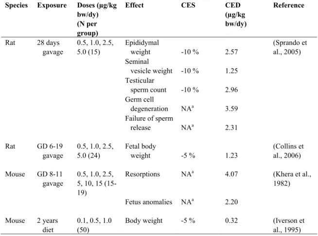
A literature review was performed to identify toxicity studies with DON. The relevant effects induced by DON included reduced body weight, toxicity to male fertility, and developmental toxicity. Three studies evaluated effects on body weight. The CED obtained for this endpoint was lowest in the study by Iverson et al. (1995). Therefore, we only used the data from Iverson regarding the effects of DON on body weight. Table 1 summarizes the relevant endpoints, which are used for dose-response analysis. Furthermore, the CES and the best estimate CED are listed for each endpoint.

Table 1. Summary of the studies used to characterize the dose-response relationships for the effects of DON. Species Exposure Doses (µg/kg

bw/dy) (N per group)

Effect CES CED

(µg/kg bw/dy) Reference Rat 28 days gavage 0.5, 1.0, 2.5, 5.0 (15) Epididymal weight -10 % 2.57 Seminal vesicle weight -10 % 1.25 Testicular sperm count -10 % 2.96 Germ cell degeneration NAa _3.59 Failure of sperm release NAa _2.31 (Sprando et al., 2005) Rat GD 6-19 gavage 0.5, 1.0, 2.5, 5.0 (24) Fetal body weight -5 % 1.23 (Collins et al., 2006) Mouse GD 8-11 gavage 0.5, 1.0, 2.5, 5, 10, 15 (15-19) Resorptions NAa_4.07 Fetus anomalies NAa_2.20 (Khera et al., 1982) Mouse 2 years diet 0.1, 0.5, 1.0 (50)

Body weight -5 % 0.32 (Iverson et

al., 1995)

a_{no CES is defined because of quantal endpoint}

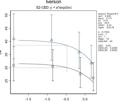
In Figure 1 the dose-response curve is given for the body weight against the dose DON. In this case an exponential model was fitted to the continuous data. As another model (Hill) is applicable too, the

(23)

distributions obtained from both models were combined to obtain an overall CED uncertainty distribution (Figure 2). -1.5 -1.0 -0.5 0.0 25 30 35 40 45 50 bw Iverson E2-CED: y = a*exp(bx) version: Proast16.3 var-f 0.408 var-m 0.171 a-f 31.6 a-m 40.5 CED-f 0.33 loglik -232.78 b: -0.1554 conv : 1 sf.x : 1 dtype : 10 selected : all CES -0.05 CED-L05 0.2208 CED-L95 0.6552

Figure 1. Dose-response of body weight (g) against log10-dose (µg/kg bw/dy). The CED (vertical dotted line)

corresponds to a CES of 5 % decrease in body weight (horizontal dotted line): triangles: males and circles: females. Data are from Iverson et al. (1995).

A) B) C)

CED (microg/kg bw/dy)

Fr eq ue nc y 0.28 0.30 0.32 0.34 0.36 0.38 0.40 0 50 10 0 150 200 25 0 300

Fr eq ue nc y 0.26 0.28 0.30 0.32 0.34 0.36 0 50 1 00 15 0 20 0 2 50

Fr eq ue nc y 0.26 0.28 0.30 0.32 0.34 0.36 0.38 0.40 0 100 20 0 30 0 40 0

Figure 2. CED distributions corresponding to a 5 % decrease in body weight. A) The distribution obtained from an exponential model model (E2). B) The distribution obtained from the Hill model (H2). C) The CED distribution obtained from combining the 2000 estimates from both models.

Extrapolation factor(s)

The animal-derived CED distributions are extrapolated to the human situation using an interspecies and intraspecies extrapolation factor. In addition, a subacute-to-chronic EF is applied to the male

(24)

fertility effects (epididymal weight, seminal vesicle weight, testicular sperm count, germ cell degeneration, and failure of sperm release).

In Table 2 the animal and human body weights are shown that are used to derive the allometric factor (according to equation (1)). When available, the animal body weights are derived from the study

reports, otherwise default body weights were applied. The body weights of the target populations are

obtained from the Dutch National Food Consumption Survey of 1997/1998 (DNFCS-3, Kistemaker et al., 1998; Voedingscentrum, 1998).

In Table 3 an overview is given of the EF distributions used to extrapolate each effect to the human situation.

Integration of the CED and EF distributions in the probabilistic risk assessment will be described in chapter 5.

Table 2. Body weight of the tested and target populations.

Endpoint Tested population Target human population

Species Sex Mean bw Age Sex Mean bw

All male fertility effects Rat M 337 g 15-45 M 80.9 kg Fetal body weight Rat F 210 g 15-45 F 69.6 kg Resorptions Mouse F 30 g 15-45 F 69.6 kg Fetus anomalies Mouse F 30 g 15-45 F 69.6 kg Body

weight Mouse M & F 49 g 1-19 M & F 33.2 kg

Table 3. EF distributions (all lognormally distributed). Effects Allometric factor Interspecies TK & TD Subacute-to-chronic P95 of intraspecies factor is between: Intraspecies All male fertility effects GM=5.2 GSD=1.2 GM=1 GSD=2 GM=4.1 GSD=4.4 2-10 GM=1 GSD=1.9 df=6.25 Fetal body weight GM=5.7 GSD=1.2

Ditto -- Ditto Ditto

Resorptions GM=10.2

GSD=1.3

Fetus anomalies

GM=10.2 GSD=1.3

Body weight GM=7.1

GSD=1.3

(25)

2.2 Effect characterization cadmium

Benchmark dose(s)

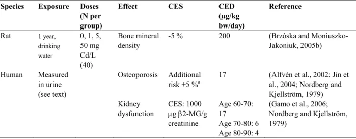
Existing risk assessment reports (e.g., JECFA, 2004) and literature were reviewed to identify the relevant endpoints and studies of cadmium toxicity. Cadmium is known to induce kidney damage, increase blood pressure, increase bone fractures (or increase osteoporosis), to alter fertility, induce tumors and cause neurobehavioral alterations in experimental animal and/or human studies. Kidney effects, which are usually the basis for human risk assessments (see e.g., JECFA, 2004), and bone effects are the most deeply investigated cadmium effects. For these two endpoints, sufficient data to derive dose-response relationships were available. Table 4 summarizes the relevant endpoints, which are used for dose-response analysis. Furthermore, the CES and the best estimate CED are listed for each endpoint.

Table 4. Summary of the studies used to characterize the dose-response relationships for the effects of cadmium.

Species Exposure Doses (N per group)

Effect CES CED (µg/kg bw/day) Reference Rat 1 year, drinking water 0, 1, 5, 50 mg Cd/L (40) Bone mineral density

-5 % 200 (Brzóska and

Moniuszko-Jakoniuk, 2005b)

Human Measured in urine (see text)

Osteoporosis Additional

risk +5 %a 17 (Alfvén et al., 2002; Jin et _{al., 2004; Nordberg and}

Kjellström, 1979) Kidney dysfunction CES: 1000 μg β2-MG/g creatinine Age 60-70: 17 Age 70-80: 6 Age 80-90: 4 (Gamo et al., 2006; Nordberg and Kjellström, 1979)

a_{the CED for the average human could not be derived for this quantal endpoint}

Kidney effects

Extensive datasets exist for cadmium-induced kidney alterations in humans. The data gathered in a meta-analysis (Gamo et al., 2006) were used to derive a dose-response relationship and obtain CED distributions for the human population. This dose-response was based on urine cadmium concentrations as a measure of dose, and urine β2-microglobulin (β2-MG) as a biomarker of adverse effects in kidney. Kidney function deteriorates with age, and consequently β2-MG levels increase with age. Therefore, a certain percent increase in β2-MG levels has different health implications at different ages. For this reason, we used a cut-off point of 1000 μg β2-MG/g creatinine instead of a percent increase to derive the CED distributions. This critical level is somewhat arbitrary but has been considered in previous work as the cut off point associated with kidney dysfunction (Gamo et al., 2006).

To compare the CED distributions obtained with dietary exposure data, the urinary cadmium concentrations were extrapolated to cadmium intake. We used the toxicokinetic model for cadmium described by Nordberg and Kjellström (1979) to derive the relationship between urinary cadmium concentration and dietary intake for the different age groups considered in the study.

(26)

In Figure 3 the concentrations of the biomarker (β2-MG) in the urine are plotted against the urinary cadmium concentrations depending on age. The fit of the model did not improve by considering sex as a covariate. 2 4 6 8 Ucad 0 500 1 000 1500 2000 2500 3000 Ub io m M

cadkidn

E3-CED: y = a*exp(bx^d) Proast16.3 var-50s 0.8291 var-60s 1.301 var-70s 2.125 var-80s 3.491 a-50s 121.2 a-60s 114.6 a-70s 115.1 a-80s 159.1 CED-50s 20060000 CED-60s 19.11 CED-70s 7.366 CED-80s 5.907 d 1 loglik -17879.13 b: 0.3361 CES : 6.28 conv : T RUE sf.x : 1 dtype : 10 selected : all fact1: age fact2: age fact3: age

Figure 3. Modeled relationship between the urinary biomarker (in μg/g creatinine) and urinary cadmium concentrations (in μg/g creatinine) based on the epidemiological data reviewed in Gamo et al. (2006). Four age groups, 50-60 years, 60-70 years, 70-80 years, and 80-90 years are indicated by circles, triangles, crosses, and diamonds, respectively.

The models fitted to the data were used to estimate the CEDs that lead to the defined cut-off point of 1000 µg β2-MG/g creatinine for each age group. The distributions of CEDs obtained are shown in Figure 4. These values, expressed as cadmium concentrations in urine, were extrapolated to long-term dietary cadmium intake using the relation between intake and urinary excretion shown in Figure 5. The best estimates (medians) of the derived CED distributions in terms of total dietary cadmium intake were: 17, 6, and 4 µg/kg bw/day for age group 60-70 years, 70-80 years, and 80-90 years, respectively.

(27)

10 15 20 25 30 0 50 100 150 200 250 300 bootstrap.cadmium.60$CED.boot 6 7 8 9 10 0 100 200 300 bootstrap.cadmium.70$CED.boot 4 5 6 7 8 9 0 50 100 150 200 bootstrap.cadmium.80$CED.boot

Figure 4. Uncertainty distributions of the dose (in terms of urine cadmium concentrations) that would lead to a urine β2-MG concentration of 1000 μg /g creatinine. From left to right: age group 60-70 years, 70-80 years, and 80-90 years.

0 5 10 15

Urine excretion (μg/day)

0 200 400 600 800 In take (μ g/ da y) 50 60 70 80 0 5 10 15

0 200 400 600 800 In take (μ g/ da y) 0 5 10 15

0 200 400 600 800 In take (μ g/ da y) 50 60 70 80

Figure 5. Long-term oral cadmium intake vs. urinary cadmium excretion for different age-groups derived from the toxicokinetic model described by Nordberg and Kjellström (1979).

Bone effects

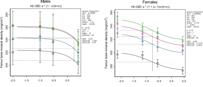
Several animal studies report dose-response data for the effects of cadmium on bone mineral density. We consider the chronic studies with male and female rats (Brzóska and Moniuszko-Jakoniuk, 2005a, b) the most relevant. These studies report the effects of cadmium on several endpoints (different measures of bone density and different bones), which showed a very similar response to cadmium exposure. Therefore, only bone mineral density in femur is used for the effect characterization. Females were considerably more sensitive than males and it was decided to limit the risk assessment to the female population (Figure 6). A dose-response model was fitted to the data. The CED distribution for a 5 % decrease in bone mineral density is derived (Figure 7). The CED distribution for the average female rat has a median of 200 µg/kg bw/day.

(28)

-2.0 -1.5 -1.0 -0.5 0.0 0.5

log₁₀(Cadmium intake in mg/kg bw)

280 300 320 340 360 F em ur bo ne m ine ral dens ity ( m g/ cm 2) Females H4-CED: a * (1 + (c-1)x/(b+x))

vers ion: Proast16.3 var-3 0.000955 a-3 301 a-6 329 a-9 341 a-12 351 CED-3 0.175 c 0.907 loglik 329.24 b: 0.15 c onv : 1 s f.x : 1 dtype : 10 s elec ted : all CES -0.05 CED-L05 0.1119 CED-L95 0.2841

-2.0 -1.5 -1.0 -0.5 0.0

log₁₀(Cadmium Intake in mg/kg bw)

300 320 340 360 380 F em ur bone m in er al d ens ity ( m g/ cm 2) Males H2-CED: a * (1 - x/(b+x))

vers ion: Proast16.3 var-3 0.00989 a-3 324 a-6 343 a-9 362 a-12 360 CED-3 1.75 loglik 142.26 b: 33.33 c onv : 1 s f.x : 1 dtype : 10 s elec ted : all CES -0.05 CED-L05 1.202 CED-L95 3.16

Figure 6. Dose-response for bone mineral density in femur (in mg/cm2_{) vs. log}₁₀_{of cadmium intake (in mg/kg}

bw/day). The circles, triangles, crosses, and diamonds indicate the dose-responses at 3, 6, 9, and 12 months after the start of the study, respectively.

0.1 0.2 0.3 0.4 0.5 0 200 400 600 800 BMD (mg/kg bw/day)

Figure 7. Uncertainty distribution for the dose associated with a 5 % decrease in femur bone mineral density in female rats.

Several human studies looking at bone effects exists. However, different endpoints were assessed and a meta-analysis similar to the one for kidney effects is therefore not feasible. We selected two epidemiological studies to see if the results as just derived from the rat data are not inconsistent with the findings in humans: Alfvén et al. (2002) and Jin et al. (2004). The first of these two studies was

(29)

also considered as the most relevant study by the EU RAR for cadmium effects on bones (EU, 2007). The second study allows the derivation of a dose-response relationship between urine cadmium concentrations and prevalence of osteoporosis for a general population environmentally exposed to cadmium in China.

The study by Alfvén et al. (2002) reported that people with blood cadmium concentrations between 5 and 10 nM have lower bone mineral densities compared to people with blood cadmium concentrations below 5 nM. The reported mean blood cadmium concentration in these two groups were 7.2 and 2.5 nM, respectively. The toxicokinetic model for cadmium described by Nordberg and Kjellström (1979) was used to derive the associated long-term cadmium intake. The blood concentration of 7.2 nM is associated to a long-term cadmium intake of approximately 2 μg/kg bw/day.

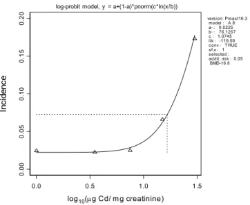
The study by Jin et al. (2004) reports the prevalence of osteoporosis in five subgroups of people with increasing urine cadmium concentrations. Dose-response models were fitted to these data and the dose associated to a 5 % increase in the prevalence of osteoporosis was derived (Figure 8). It may be noted that another option would be to follow an approach for quantal data that better matches the CES as defined for continuous data, as discussed in, e.g., Bos et al. (2009). Indeed, it may be argued that this approach is preferable for the purpose of comparing the final risk outcomes related to continuous vs. quantal data.

The urine concentration with a median of 17 µg cadmium per g creatinine associated to the 5 % increased incidence was extrapolated to a long-term cadmium intake using the toxicokinetic model for cadmium described by Nordberg and Kjellström (1979). This urine cadmium concentration is associated to a long-term cadmium intake of approximately 1.2 mg/kg bw/day.

0.0 0.5 1.0 1.5 log₁₀(μg Cd/ mg creatinine) 0. 00 0. 05 0. 10 0. 15 0. 20 In ci de nc e

log-probit model, y = a+(1-a)*pnorm(c*ln(x/b))

version: Proast16.3 model : A 8 a- : 0.0225 b- : 76.1257 c : 1.0745 lik : -119.59 conv : T RUE sf.x : 1 selected : addit. risk : 0.05 BMD-16.6

Figure 8. Dose-response for osteoporosis prevalence as a function of urinary cadmium concentration. Data are from Jin et al. (2004).

The two benchmark exposures in these two epidemiological studies are quite different. However, they are not directly comparable. First of all, osteoporosis may be regarded as a severe stage of low bone

(30)

mineral density (WHO, 2003). Therefore it is not surprising that the benchmark exposure is higher when obtained from an increased prevalence of osteoporosis as compared to being based on a statistically significant decrease in bone mineral density. Another reason for obtaining different benchmark exposures is the different experimental setup of the Jin and Alfvén studies: the biomarkers are measured in different matrixes (blood vs. urine) and different subpopulations (Swedish vs. Chinese).

The best estimate of the dose associated to a 5 % decrease in bone mineral density in the animal study is 200 µg/kg bw/day, which is in the range of the benchmark exposures derived from the human

studies1_.

The rat derived CED distribution for bone mineral density is extrapolated to the human situation using an interspecies and intraspecies extrapolation factor.

In Table 5 the rat and human body weights are shown that are used to derive the allometric factor (according to equation (1)). The animal body weight is derived from the study report. The body weights of the target populations are obtained from DNFCS-3.

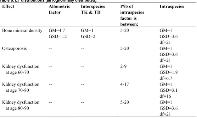
In Table 6 an overview is given of the applied EF distributions. The CED distributions for osteoporosis and kidney dysfunction are obtained from human studies. Therefore, no interspecies extrapolation is applied. The variances obtained when modeling the dose-response relationships for each of the age groups in the epidemiological data were used as an indication of the differences between sensitive and average humans. These values were considered as the upper bound of these possible differences because the experimental variances are likely to reflect other factors in addition to differences in sensitivity. The lower bound of these possible differences was estimated to be four-fold lower than the upper bound.

Integration of the CED and EF distributions in the probabilistic risk assessment will be described in chapter 5.

Effect Tested population Target human population

Species Sex Mean bw

(kg)

Age Sex Mean bw

(kg)

Bone mineral density Rat F 0.35 15-20 F 61

Osteoporosis Human (Asian)

M&F 56 kg 20-70 M&F 56 kg

Kidney dysfunction

age group 60-70 Human M&F 56 kg 20-70 M&F 56 kg

Kidney dysfunction

(31)

Table 6. EF distributions (all lognormally distributed). Effect Allometric factor Interspecies TK & TD P95 of intraspecies factor is between: Intraspecies

Bone mineral density GM=4.7 GSD=1.2 GM=1 GSD=2 5-20 GM=1 GSD=3.6 df=21 Osteoporosis -- -- 5-20 GM=1 GSD=3.6 df=21 Kidney dysfunction at age 60-70 -- -- 2-9 GM=1 GSD=1.9 df=6.7 Kidney dysfunction at age 70-80 -- -- 4-17 GM=1 GSD=3.1 df=16 Kidney dysfunction at age 80-90 -- -- 5-20 GM=1 GSD=3.6 df=21

2.3 Effect characterization OPs

Benchmark dose(s)

The critical effect under consideration is inhibition of AChE in the brain. This is a transient, reversible effect due to reactivation and de novo synthesis of AChE. The pattern of exposure (dose, composition and frequency) determines the time course of inhibition. It is not fully understood how the time course of inhibition relates to adverse symptoms of cholinergic crisis (peak, prolonged inhibition, or a combination of both), but it is generally assumed that inhibition below 20 % does not cause adverse symptoms. Therefore, the CES used here is a decrease of 20 % in brain AChE activity.

Residues of 30 different OPs have been found in samples of Dutch food items. For 15 of these OPs, dose response-data were provided by US EPA, mostly (semi)chronic repeated dose studies (Table 1), and for these 15 OPs we derived the CEDs. There is a discrepancy between animal and human exposure patterns: animals receive a constant daily dose of a single OP, whereas humans may be exposed irregularly to a variety of OPs. We made two conservative assumptions:

• All OPs ingested by humans on the same day are ingested at the same time.

• Dose-response data from repeated dose studies were used as surrogate for acute effects. We

assumed that steady-state inhibition after repeated doses is not much higher than the maximum inhibition after exposure to a single dose.

For the remaining 15 OPs in the residue concentration database (those for which no EPA data were available), we obtained a point of departure from descriptions of toxicity studies in the JMPR monographs (2008), serving as a surrogate for the CED.

(32)

Relative Potency Factors

In the RPF approach, doses of all chemicals are expressed as equivalents of one of them: the index chemical. The effect of the combination equals that of the sum of the equivalents of the index chemical. This method requires:

• the same target/effect – it is assumed that OPs inhibit AChE by a common mechanism;

• no interactions between the chemicals – no clear evidence of interactions has been found in

several mixture studies;

• parallel dose-response curves – this will be verified by analysis of dose-response data.

For the OPs for which we have dose-response data, parallel dose-response functions were fit to the data for all OPs simultaneously using the software PROAST (Slob, 2002).

The available dose-response data could indeed be described well by parallel dose-response curves (See below). The only exception was malathion, which appeared to have a more shallow dose-response. Its relative potency is however so low that the contribution to the cumulative effect may be negligible. This will be verified by the exposure assessment below.

In the toxicity studies some differences in sensitivity between males and females were observed. Overall, females appeared to be slightly more sensitive than males, but not consistently. No information is available showing that this difference is a true sex related effect relevant to humans. The female data are used to estimate RPFs and the CED of the index chemical. Methamidophos is used as the index OP. In theory, the arbitrary choice of the index chemical should not affect the results. Bosgra et al. (in press) confirmed this by repeating the calculations acephate as index OP.

The upper panel of Figure 9 shows the simultaneous fit of the dose-response curves related to the 15 OPs. There were considerable differences in background AChE levels between the studies (hence between the OPs). Data were re-scaled to the dose-response curve of methamidophos by correcting for differences in background AChE levels, resulting in the lower left panel in Figure 9. This results in this figure were used to estimate the RPFs. Next, the dose-response data were corrected for the differences in potency, i.e., the RPFs for each OP. This resulted in the lower tight panel of Figure 9, and from this analysis the distribution for the CED (at 20 % inhibition) for the index chemical was derived.

(33)

-4 -3 -2 -1 0 1 2 log10- dose 01 0 20 30 ch e .m y = a * [c - (c-1)exp(-(x/b))] (-Inf) (-Inf) (-Inf) (-Inf) (-Inf) (-Inf) (-Inf) (-Inf) (-Inf) (-Inf) (-Inf) (-Inf) (-Inf) (-Inf) (-Inf) (-Inf) -4 -3 -2 -1 0 1 2 log10- dose 51 0 15 m.m m p y = a * [c - (c-1)exp(-(x/b))] (-Inf) (-Inf) (-Inf) (-Inf) (-Inf) (-Inf) (-Inf) (-Inf) (-Inf) (-Inf) (-Inf) (-Inf) (-Inf) (-Inf) (-Inf) (-Inf) -4 -3 -2 -1 0 1 log10- dose 51 0 15 ch e .m y = a * [c - (c-1)exp(-(x/b))] (-Inf)

Figure 9. Upper panel: dose-response data of 15 OPs from the US EPA database described by the same fitted model, taking differences in background response and in potency into account (parameters a and b, respectively). Lower left panel: dose-response data vertically re-scaled to the background AChE level in the dataset of the index chemical (methamidophos). Lower right panel: data horizontally scaled by correcting for the relative potency of each OP.

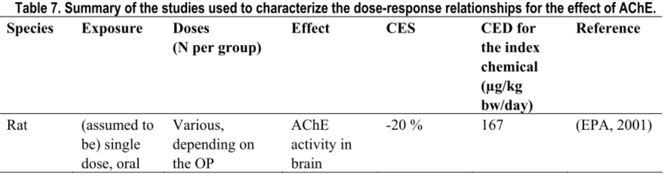
Table 7. Summary of the studies used to characterize the dose-response relationships for the effect of AChE. Species Exposure Doses

(N per group)

Effect CES CED for

the index chemical (µg/kg bw/day) Reference Rat (assumed to be) single dose, oral Various, depending on the OP AChE activity in brain -20 % 167 (EPA, 2001)

(34)

For the remaining 15 OPs no dose-response data were available. Estimates of the RPFs for these OPs were derived from a reference point on the dose-response curve as reported in the JMPR monographs, under the assumption that their dose-response curves are parallel (on log-dose scale) to those for which we do have dose-response data. For the purpose of comparison the CEDs corresponding to 20 % inhibition are estimated for these OPs Table 8 (Bosgra et al., in press).

Table 8. Estimates of the CED corresponding to a 20 % decrease in AChE activity of 30 OPs found in food samples from the Dutch market and RPFs with MMP as index OP.

OP CED (mg/kg bw) RPF (MMP as index) Acephate* (ACP) 4.41 0.036 Azinphos-methyl* 0.48 0.33 Bromophos-ethyl (6.44) 0.025 Chlorfenvinphos (0.53) 0.30 Chlorpyrifos* 2.58 0.062 Chlorpyrifos-methyl* 16.6 0.0096 Diazinon* 5.15 0.031 Dichlorvos* 4.65 0.034 Dimethoate* 1.26 0.13 Ethion (0.15) 1.07 Fenitrothion (1.54) 0.10 Fenthion* 0.51 0.31 Heptenophos (1.07) 0.15 Mecarbam (0.45) 0.36 Methamidophos* (MMP) 0.16 1 Methidathion* 1.03 0.16 Mevinphos* 0.17 0.93 Monocrotophos (0.031) 5.17 Omethoate (0.11) 1.50 Parathion 0.86) 0.19 Parathion-methyl* 0.82 0.20 Phosalone* 5.95 0.027 Phosmet* 2.28 0.070 Pirimiphos-ethyl (0.17) 0.93 Pirimiphos-methyl* 3.57 0.045 Profenphos (42.9) 0.0037 Pyrazophos (4) 0.045 Quinalphos (6.44) 0.025 Tolclofos-methyl (1494) 0.00011 Triazophos (28) 0.0057

For OPs marked with an asterix dose-response data were available. For the remaining OPs, JMPR monographs (2008) were used to estimate the RPF. The estimated CEDs of these OPs are shown within brackets.

The CED distribution for AChE activity related to the index chemical is extrapolated to the human situation using an interspecies and intraspecies extrapolation factor. It is assumed that the RPFs as

(35)

estimated in the rat are equal in humans (relative to the human CED of the index chemical). Default rat and human body weight are used to derive the allometric factor according to equation (1) (Table 9). In Table 10 an overview is given of the EF distributions used to extrapolate the point of departure to the human target population. Integration of the CED and EF distributions in the probabilistic risk assessment is described in chapter 5.

Species Sex Mean bw Age (yr) Sex Mean bw

AChE Rat-7wk F 0.3 16 F 70

Table 10. EF distributions (all lognormally distributed) Effects Allometric fact Interspecies TK & TD P95 of intraspecies factor is between: Intraspecies AChE GM=5.1 GSD=1.2 GM=1 GSD=2 2-10 GM=1 GSD=1.9 df=6.25

2.4 Effect characterization T-2/HT-2

Benchmark dose(s)

The immunotoxicity data in the studies from Rafai and Meissonnier were used to perform the probabilistic risk assessment. It should be noted that other studies (Faifer et al., 1992; Hayes et al., 1980; Ohtsubo and Saito, 1977; Rousseaux et al., 1986; Rukmini et al., 1980; Schiefer et al., 1987; Schoental et al., 1979; Sirkka et al., 1992; Smith et al., 1994; Ueno, 1984; Velazco et al., 1996) were examined on useful toxicity data. However, these studies did not provide data in enough detail for effect characterization.

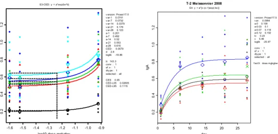
Figures 10 and 11 show the dose response curves of the data from Rafai and Meissonnier, respectively. Figure 11 shows that the highest dose of T-2/HT-2 results in an increased IgA concentration already after one day, an acute effect that remains over time without increasing in strength.

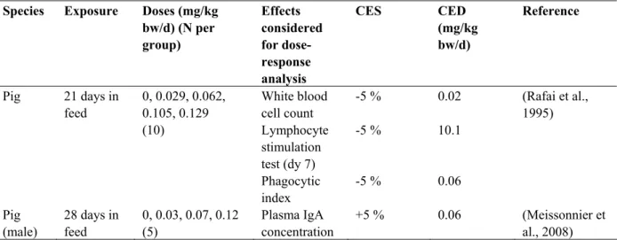
Table 11 shows the summary of the studies used to characterize the dose-response relationships for the toxic effects of T-2/HT-2.

(36)

Table 11. Summary of the studies used to characterize the dose-response relationships for the effects of T-2/HT-2.

Species Exposure Doses (mg/kg bw/d) (N per group) Effects considered for dose-response analysis CES CED (mg/kg bw/d) Reference White blood cell count -5 % 0.02 Lymphocyte stimulation test (dy 7) -5 % 10.1 Pig 21 days in feed 0, 0.029, 0.062, 0.105, 0.129 (10) Phagocytic index -5 % 0.06 (Rafai et al., 1995) Pig (male) 28 days in feed 0, 0.03, 0.07, 0.12 (5) Plasma IgA concentration +5 % 0.06 (Meissonnier et al., 2008)

(37)

-1.6 -1.4 -1.2 -1.0 10 12 14 16 18 log10-dose.mgkgbw wb c. m E2-CED: y = a*exp(bx) v ersion: Proast17.5 v ar- 0.0268 a- 15.8 CED- 0.0169 loglik 19.51 b: -3.027 conv : 1 sf .x : 1 dty pe : 10 selected : all CES -0.05 CED-L05 0.01335 CED-L95 0.02318 -1.6 -1.4 -1.2 -1.0 5 10 15 202 53 0 35 log10-dose.mgkgbw AH G LS T .m Rafai1995 E2-CED: y = a*exp(bx) v ersion: Proast17.5 v ar-7 0.532 v ar-14 0.145 v ar-21 0.113 a-7 10.1 a-14 20.5 a-21 23.3 CED-7 0.0115 CED-14 0.0144 CED-21 0.00656 loglik -94.22 b: -4.474 b: -3.569 b: -7.818 conv : 1 sf .x : 1 dty pe : 10 selected : all CES -0.05 CED-L05 0.006331 CED-L95 0.06179 CED-L05 0.009384 CED-L95 0.03073 CED-L05 0.005405 CED-L95 0.008347 -1.6 -1.4 -1.2 -1.0 3.0 3.5 4.0 4.5 5.0 5.5 log10-dose.mgkgbw pha gi nd. m Rafai1995 E2-CED: y = a*exp(bx) v ersion: Proast17.5 v ar- 0.0545 a- 4.02 CED- 0.0631 loglik 5.32 b: -0.8123 conv : 1 sf .x : 1 dty pe : 10 selected : all CES -0.05 CED-L05 0.03477 CED-L95 0.3513

Figure 10. Dose-responses of white blood cell count (WBC), lymphocyte stimulation (AHGLST), and phagocytic index (PI) against log10 of dose (mg/kg bw/d). The latter two endpoints were measured three times during the

study; at day 7 (circles), 14 (triangles), and 21 (crosses). The curve for the phagocytic index is the same at each measuring time.

(38)

-1.6 -1.5 -1.4 -1.3 -1.2 -1.1 -1.0 -0.9 0. 20 .40 .60 .81 .0 1. 2 log10-dose.mgkgbw Ig A E3-CED: y = a*exp(bx^d) v ersion: Proast17.5 v ar-1 0.0741 v ar-7 0.0732 v ar-14 0.0379 v ar-21 0.179 v ar-28 0.123 a-1 0.201 a-7 0.492 a-14 0.52 a-21 0.553 a-28 0.615 CED- 0.0579 d 2.8 loglik -18.86 b: 143.3 conv : 1 sf .x : 1 dty pe : 1 selected : all CES 0.05 CED-L05 0.02605 CED-L95 0.1115 0 5 10 15 20 25 0.2 0.4 0.6 0.8 1.0 1.2 day Ig A T-2 Meissonnier 2008 E4: y = a*[c-(c-1)exp(-bx)] v ersion: Proast17.5 v ar- 0.0984 a-0 0.108 a-0.03 0.1 a-0.07 0.118 a-0.12 0.152 b- 0.23 c 5.46 loglik -25.97 conv : 1 sf .x : 1 dty pe : 1 selected : all f act3: dose.mgkgbw

Figure 11. Left: Plot of plasma IgA concentration against log10 dose (mg/kg bw/d). IgA was measured five times

during the study; at day 1 (O), 7 (Δ), 14 (×), 21 (◊), and 28 (∇).

Right: Same data, with day of measurement on the x-axis, and dose as the covariate, with dose (mg/kg bw/d) levels: 0 (O), 0.03 (Δ), 0.07 (×), and 0.12 (◊)

In the left panel, parameter b is not significantly different among observation times (log-likelihood ratio test; see Slob, 2002), which indicates that the strength of the response does not increase over time (i.e., dose-response curves are parallel on log-IgA scale).

The animal-derived CED distributions are extrapolated to the human situation using an interspecies and intraspecies extrapolation factor.

In Table 12 the animal and human body weights are shown that are used to derive the allometric factor (according to equation (1)). When available, the animal body weights are derived from the study reports, otherwise default body weights were applied. The body weights of the target populations are obtained from DNFCS-3.

Integration of the CED and (other) EF distributions in the probabilistic risk assessment will be described in chapter 5.

Species Age Mean bw

(kg)

Age Sex Mean bw

White blood cell count Lymphocyte stimulation test Phagocytic index pig 1-2 months 18.4 1-4 Not specified 14.5 Plasma IgA concentration pig 1-2 months 30 1-4 M 14.5

(39)

Table 13: EF distributions (all lognormally distributed). Effect Allometric factor Interspecies TK & TD P95 of intraspecies factor is between: Intraspecies

White blood cell count Lymphocyte stimulation test Phagocytic index GM=0.93, GSD=1.0 GM=1.0, GSD=2.0 2-10 GM=1.0 GSD=1.9 df=6.25 Plasma IgA concentration GM=0.8, GSD=1.0 GM=1.0, GSD=2.0 2-10 GM=1.0 GSD=1.9 df=6.25

2.5 Effect characterization acrylamide

Benchmark dose(s)

A literature review was performed to identify toxicity studies with acrylamide. The relevant effects induced by acrylamide included neurotoxicity as measured by grip strength. Data on carcinogenicity were not obtained since the current probabilistic approach was not developed for assessing carcinogenicity (see Discussion). Other endpoints that showed dose-related effects were the number of life pups/litter and body weight gain. The quantal effect ‘life pups/litter’ was analyzed as continuous data since the appropriate data to express the life pups/litter in a fraction of the total number of implantation sites were not available. The dose-response data of these endpoints are shown in Figure 12. Table 14 summarizes the relevant endpoints and the key studies. Furthermore, the CES and

(40)

A) B) -2.0 -1.5 -1.0 -0.5 0.0 11 12 13 14 15 log10-dosemgkgbw LP L. m chapin1995 E2-CED: y = a*exp(bx) v ersion: Proast17.5 v ar- 0.0343 a- 13.5 CED- 1.04 loglik 25.91 b: -0.04951 conv : 1 sf .x : 1 dty pe : 10 selected : generation P CES -0.05 CED-L05 0.5777 CED-L95 5.119 -2.0 -1.5 -1.0 -0.5 0.0 6 8 10 12 14 16 18 log10-dosemgkgbw LP L. m chapin1995 E2-CED: y = a*exp(bx) v ersion: Proast17.5 v ar- 0.0968 a- 14.6 CED- 0.155 loglik -16.35 b: -0.3302 conv : 1 sf .x : 1 dty pe : 10 selected : generation F1 CES -0.05 CED-L05 0.1265 CED-L95 0.2013 C) D) -2.0 -1.5 -1.0 -0.5 0.0 75 80 85 90 95 100 105 log10-dosemgkgbw F1 G S f. m chapin1995 E4-CED: y = a * [c-(c-1)exp(-bx)] v ersion: Proast17.5 v ar- 0.0198 a- 97.1 CED- 0.136 c 0.845 loglik 21.66 b: 2.861 conv : 1 sf .x : 1 dty pe : 10 selected : all CES -0.05 CED-L05 0.04711 CED-L95 0.6684 -2.0 -1.5 -1.0 -0.5 0.0 0.5 80 100 120 140 160 180 200 log10-dosemgkgbw BW g. m Tyl2000 E4-CED: y = a * [c-(c-1)exp(-bx)] v ersion: Proast17.5 v ar-f 0.00649 v ar-m 0.0127 a-f 81.5 a-m 195 CED- 0.674 c 0.902 loglik 223.45 b: 1.057 conv : 1 sf .x : 1 dty pe : 10 selected : generation P CES -0.05 CED-L05 0.2926 CED-L95 1.57

Figure 12. Dose-responses of A) life pups per litter of the P generation, B) life pups per litter of the F1 generation, C) forelimb grip strength of the F1 generation, and D) body weight gain of the P generation (triangles: males, circles: females).

(41)

Table 14. Summary of the studies used to characterize the dose-response relationships for the effects of acrylamide.

Species Exposure Doses (mg/kg bw) (N per Group) Effect considered for dose-response analysis CES CED (mg/kg bw) Reference Mouse F1 live pups/litter -5 % 0.16 Mouse F1 grip strength forelimb -5 % 0.14 Mouse 2-generations, drinking water 0, 3, 10, 20 ppm (40, 20, 20, 20/sex) P live pups /litter -5 % 1.04 (Chapin et al., 1995) Rat 2-generations, drinking water 0, 0.5, 2.0, 5.0 mg/kg bw/d (30/sex)

P BW gain -5 % 0.67 (Tyl et al.,

2000)

The animal derived CED distributions are extrapolated to the human situation using an interspecies and intraspecies extrapolation factor.

In Table 15 the animal and human body weights are shown that are used to derive the allometric factor (according to equation (1)). When available, the animal body weights are derived from the study reports, otherwise default body weights were applied. The body weights of the target populations are obtained from DNFCS-3.

Integration of the CED and EF distributions in the probabilistic risk assessment will be described in Chapter 5.

Species Sex Mean bw Age Sex Mean bw

F1 live pups/litter mouse F 0.03 15-45 F 67.3 mouse M 0.03 all M 63 F1 grip strength forelimb mouse F 0.03 all F 57.8 P live pups/litter mouse F 0.03 15-45 F 67.3 P BW gain rat M 0.25 1-19 M 34.1

(42)

Table 16. EF distributions (all lognormally distributed).

Effect Allometric factor Interspecies TK & TD P95 of intraspecies factor is in the range: Intraspecies F1 live pups/litter GM=10.1 GSD=1.3 GM=1.0, GSD=2.0 2-10 GM=1.0 GSD=1.9 df=6.25 F1 grip strength forelimb M GM=9.9 GSD=1.3 F GM=9.7 GSD=1.3

P live pups /litter GM=10.1

GSD=1.3 GM=1.0, GSD=2.0 2-10 GM=1.0 GSD=1.9 df=6.25 P BW gain M GM=4.4 GSD=1.2 F GM=5.0 GSD=1.2 GM=1.0, GSD=2.0 2-10 GM=1.0 GSD=1.9 df=6.25

(43)