Deep Learning for Computer-Aided Diagnosis of Lung Nodules in low-dose CT scans

Lung Nodules in low-dose CT scans

Academic year 2019-2020

Master of Science in Biomedical Engineering

Master's dissertation submitted in order to obtain the academic degree of

Counsellor: Milan Decuyper

Supervisor: Prof. dr. Roel Van Holen

Student number: 01507095

Nathan Sennesael

Lung Nodules in low-dose CT scans

Academic year 2019-2020

Master of Science in Biomedical Engineering

Master's dissertation submitted in order to obtain the academic degree of

Counsellor: Milan Decuyper

Supervisor: Prof. dr. Roel Van Holen

Student number: 01507095

Nathan Sennesael

The author gives permission to make this master dissertation available for consultation and to copy parts of this master dissertation for personal use. In all cases of other use, the copyright terms have to be respected, in particular with regard to the obligation to state explicitly the source when quoting results from this master dissertation.

A little over a year ago, with very little knowledge and experience in computer program-ming, I chose this topic for my master’s dissertation. I did this for two reasons: because I very much enjoy learning completely new skills and because I read a lot about the impressive achievements of artificial intelligence in recent years. I found this project to be tremendously challenging and it has truly been one of the most educative experiences of my life thus far.

I would like to express my utmost gratitude to my promoter; Prof. dr. Roel Van Holen, and counsellor; Ir. Milan Decuyper, for providing me with the tools and freedom that made this master’s dissertation possible. I would like to specifically thank Milan again for his guidance, insights and critical feedback that helped improve this thesis.

Furthermore, I want to thank: my girlfriend for her limitless love and support, Apr. Jens Helskens for his friendship and the many memories we made together throughout our studies, my parents for providing me with the gift of life and my grandmother for her endless nurture.

This list could easily be continues beyond the peripheries of this pages. However, I can’t help but think of the ”butterfly effect” when coming up with where my gratitude is due. Our world is such a complex system, that even the most minutiae changes on the other side of the world could have made a significant impact on the outcome of this thesis. In that spirit, I would like to thank not just every single human, but every living thing, every molecule, subatomic particle, every piece of space-time, energy-mass and finally the laws that govern all of those. With that, I’m confident I didn’t forget to thank anyone/anything.

Nodules in low-dose CT scans

Nathan Sennesael

Student number: 01507095

Promoter: Prof. dr. Roel Van Holen Counsellor: Ir. Milan Decuyper

Master’s dissertation submitted in order to obtain the academic degree of Master of Science in Biomedical Engineering Academic year: 2019 – 2020

Abstract_{- Cancer is globally the second most common cause of death. Lung cancer specifically, is} the most common cause of cancer death due to high prevalence and mortality rates. Lung cancer has a 5-year survival rate of only 20% when receiving general treatment. However, if lung cancer is detected at an early stage (localized), the 5-year survival rate is increased to approximately 55%. To improve the survival chances of patients, screening using low-dose Computed Tomography (CT) scans in high-risk population groups has increasingly become routine practice. The analysis of these scans is a time-consuming and tedious process, resulting in a high workload for radiologists. In recent years, a new Artificial Intelligence (AI) technique known as Deep Learning (DL) of Artificial Neural Networks (ANNs) has shown tremendous effectiveness in a variety of applications, including radiology. What is revolutionary about these techniques is that the ANNs learn by themselves which features of the CT scans are most important, as apposed to classical techniques in which the features had to be handcrafted and hard-coded. In this thesis, 3D U-Nets are trained for the detection and segmentation of lung nodules. These nodule detectors are evaluated based on total Dice score (a.k.a. F1 score) on the scan-level as a function of the applied threshold and the sensitivity as a function of the amount of false positives after thresholding. The initial nodule detector obtained a maximal Dice score of 35.9% and a maximal sensitivity of 95.6%. After adaptations, the most accurate nodule detector achieved a maximal Dice score of 43.4% and a maximal sensitivity of 96.2%. An additional CNN is applied in series to reduce false positives of the nodule detector. The maximal Dice coefficient of the initial detector was increased by 10.8% while the sensitivity is unaffected. Finally, a CNN is trained to determine whether the considered nodules are malignant or benign, providing diagnostic information on top of detection and segmentation of the nodules.

Lung Nodules in low-dose CT scans

Nathan Sennesael

Promotor: Prof. dr. Roel Van Holen Counsellor: Ir. Milan Decuyper

Abstract—Cancer is globally the second most common cause of death. Lung cancer specifically, is the most common cause of cancer death due to high prevalence and mortality rates. Lung cancer has a 5-year survival rate of only 20% when receiving general treatment. However, if lung cancer is detected at an early stage (localized), the 5-year survival rate is increased to approximately 55%. To improve the survival chances of patients, screening using low-dose Computed Tomography (CT) scans in high-risk population groups has increasingly become routine practice. The analysis of these scans is a time-consuming and tedious process, resulting in a high workload for radiologists. In recent years, a new Artificial Intelligence (AI) technique known as Deep Learning (DL) of Artificial Neural Networks (ANNs) has shown tremendous effectiveness in a variety of applications, including radiology. What is revolutionary about these techniques is that the ANNs learn by themselves which features of the CT scans are most important, as apposed to classical techniques in which the features had to be handcrafted and hard-coded. In this thesis, 3D U-Nets are trained for the detection and segmentation of lung nodules. These nodule detectors are evaluated based on total Dice score (a.k.a. F1 score) on the scan-level as a function of the applied threshold and the sensitivity as a function of the amount of false positives after thresholding. The initial nodule detector obtained a maximal Dice score of 35.9% and a maximal sensitivity of 95.6%. After adaptations, the most accurate nodule detector achieved a maximal Dice score of 43.4% and a maximal sensitivity of 96.2%. An additional CNN is applied in series to reduce false positives of the nodule detector. The maximal Dice coefficient of the initial detector was increased by 10.8% while the sensitivity is unaffected. Finally, a CNN is trained to determine whether the considered nodules are malignant or benign, providing diagnostic information on top of detection and segmentation of the nodules.

I. INTRODUCTION

Cancer is globally the second most common cause of death, only preceded by cardiovascular disease. Lung cancer specifically, is the most common cause of cancer death due to high prevalence and mortality rates. Upon diagnosis and with general treatment, lung cancer has a 5-year survival rate of only 20%. However, when lung cancer is detected at an early stage (localized), the 5-year survival rate is increased to approximately 55%. Additionally, other respiratory diseases, such as lung infections (e.g. COVID-19), account for the third most common cause of death globally. Generally, lungs are a sensitive organ, which makes diagnosis and treatment of lung cancer particularly difficult. As of today, lung cancer and other pathologies of the lung still pose a major challenge for the medical field.

In an effort to reduce the burden, lung cancer screening has increasingly become routine practice in high risk population groups. As a result of various anatomical aspects of the lungs, one of the only practical methods for diagnosis of lung cancer is the use of radiographs and Computed Tomography (CT) scans. Unfortunately, the lungs are also some of the most radio-sensitive organs in the human body. Therefore, low-dose CT scans are used for lung cancer screening. As a result, the signal-to-noise ratio and image quality is significantly lowered [1].

An important step in the diagnosis of lung cancer is the detection of pulmonary nodules (a.k.a. lung nodules, spots or lesions). A pulmonary nodule is a small round or oval-shaped growth in the lung. Lung nodules show large variations in shape, size and appearance. Additionally, nodules often look similar to the neighbouring bronchi in a single slice of the CT scan. Together with the low image quality, this makes the detection of lung nodules is a time-consuming and tedious task, resulting in a heavy workloads for radiologists.

For many years, computers have been used to try and de-velop Compute-Aided-Diagnosis (CAD) systems which could help reduce this workload. In recent year, the field of Arti-ficial Intelligence (AI) has shown tremendous advances and impressive results in a variety of applications. This is because of a new Machine Learning technique (ML) known as Deep Learning (DL), which uses deep Artificial Neural Networks (ANNs) to construct a mathematical model which can compute the desired output for the given task. These type of CAD systems have a significant advantage because they learn them-selves which features are most important, as apposed to classic methods in which this has to be manually encoded.

Deep Learning CAD systems have shown the potential to perform the detection of lung nodules more accurately and consistently than radiologists. Additionally, (at least partial) automation of this task could save time and significantly reduce hospital expenses. Despite these promising results, computers will most likely not fully autonomously perform this task without revision of radiologists in clinical practice any time soon.

The objective of this thesis is the development develop a CAD system with the focus on aiding the radiologist in detection, segmentation and diagnosis of nodules. A specific type of ANNs is used to achieve this, known as

detection and segmentation. However, this model generated a large amount of false positives. Therefore a second CNN is applied in series to reduce the amount of false positives in the output of the detector. Finally, a CNN is trained on the malignancy scores of nodules. This allows radiologists to be provided with diagnostic information on top of the location and segmentation of the nodules.

II. MATERIALS

A. Database

Since supervised deep learning techniques are used, large quantities of data are required to train the ANNs.

The Lung Image Database Consortium and Image Database Resource Initiative (LIDC-IDRI) is a publicly available refer-ence data base for the medical imaging research community [2]. The LIDC-IDRI Database contains 1018 cases, each of which includes images from a clinical thoracic CT scan and associated files that records the results of annotation performed by four experienced thoracic radiologists. Nodules > 3mm (3–30mm) are the main focus of the database, smaller lesions are of lesser clinical relevance.

Besides the segmentations performed by the radiologists, the dataset also contains other interesting information such as the age and gender of the patients. Additionally each nodule contains information about: subtlety (difficulty of detection), internal structure (soft tissue, fluid, fat or air), degree of calcification, sphericity, lobulation (how well defined the boundaries of the nodule are), spiculation, texture & malignancy.

B. Hardware & Software

All code is written in python and will be made available on the public github repository [3]. All neural networks were constructed with the use of the Keras and TensorFlow open-source libraries.

The majority of results were obtained with the use of an Ubuntu server provided by the Medical Image and Signal Processing (MEDISIP) research group at Ghent University. Training of the ANNs was done using the NVIDIA GeForce GTX 1080 Ti GPU. The server also contained an Intel R

CoreTM i7-7820X CPU.

III. PRE-PROCESSING

The scans are provided in DICOM (Digital Imaging and COmmunications in Medicine) format and the annotations are in XML format which are converted to numpy arrays for processing in Python. The dataset contains the individual an-notations of the four radiologists. To maximize the sensitivity of the eventual network, the union of all four segmentation masks is used as ground truth.

figure 1:

Fig. 1. Pre-processing of CT-scans

1) First the value of air is determined by taking the average of a few values at the center of the very top of the CT scan. All the array values close to this value are set to zero, improving the contrast of the scan.

2) The array is first normalized to ensure the segmentation algorithm works on as many scans as possible. The lungs are segmented by considering the largest enclosing volume in the array below a certain threshold value. Finally a binary dilation algorithm is applied to make sure the edges of the lung are captured. This is necessary since lung nodules in contact with the edge would otherwise be considered as soft tissue and would be removed by the algorithm.

3) This segmentation mask is simply multiplied element-wise with the original CT scan array.

4) The high values in the histogram of the array are removed through an upper threshold to increase the con-trast of the important features in the lungs. Afterwards, the array is normalized once more.

5) Finally the scans are cropped such that all the unnec-essary zeros are removed. Thus, the dimensions of the array are set to match the dimensions of the lungs.

.

The pre-processing algorithm worked successfully on the great majority of scans, however, as a result of artifacts and noise (and others) it did not succeed on all scans in the database. Therefore, several scans were purposely left out due to their poor quality.

The data is split into training (80.0%), validation (8.2%) and testing (11.7%) data on the scan-level. The training data consists of 683 scans, the validation data of 70 scans and test data consists of 100 scan, equating to a total of 853 scans.

segments the nodules in the scan along with many other structures (primarily blood vessels), which the model may have mistaken for nodules. Several nodule detectors are trained with different adaptations in: augmentation, architecture, input data shape. These different models are evaluated and compared.

A. Box Extraction & Reconstruction

The CT scan arrays have dimensions_{512 × 512 × z, where} z differs between scans but usually has a value between 50 and 300. To prevent the memory from being overloaded, and to increase the sentivity of the model, the network is trained on smaller box as apposed to entire scans. The size of the boxes was chosen to be large enough such that it is able to fully encapsulate the great majority of lung nodules. Two box sizes were tested, _{64 × 64 × 16 and 32 × 32 × 16, see figure} 2.

Fig. 2. Capture nodules in boxes

After training a nodule detector on a set of extracted boxes, the model is evaluated by letting it make predictions on boxes it has never seen before. This was systematically done by subdividing entire scans into overlapping boxes.

The stride was chosen to be1/4 of each respective dimen-sion of the box such that the great majority of nodule is fully encapsulated in at least one box, see figure . A smaller stride generally results in a more accurate and smooth final output.

Fig. 3. Overlapping extraction & reconstruction

The overlapping predictions are summed up into one array, analogous (but reversely) to how the original input scan was

to the interval [0, 1], this allows the final output to again be interpreted as a probability.

B. Training Data

In order to synthesize a dataset that can be used to train the model, homogeneously extracting boxes from the scans does not suffice. This would result in the great majority of boxes not containing any nodules. such unbalanced data would make it very difficult to properly train a model.

This is generally solved by undersampling the majority class (non-nodule containing boxes) and/or oversampling the minority class (nodule containing boxes).

Several trial runs showed that adding non-nodule containing boxes in the training set only negatively impacted the results obtained by the model. Based on this observation, only nodule containing boxes were further used to train the nodule detec-tors.

In total there is 5,797 original samples (non-augmented nodule-containing boxes) in the 753 training+validation scans. Oversampling of nodule-containing boxes was never per-formed through exact duplicates, instead, the nodules were captured at different translational views (similar as in in figure 3) or other augmentations.

C. Augmentations

Besides the different translational views, additional augmen-tations were applied to increase the size of the training dataset, this was only done for boxes of size_{64 × 64 × 16.}

The following augmentation techniques will be used: dif-ferent views (translations), rotations , flips (mirrors). More precisely, four models were trained under the exact same conditions, with the only difference being the data they are trained upon.

• Model 0: two translational views of each nodule • Model 1: two translational and one central view • Model 2: four translational and one central view

• Model 3: four translational and one central view

+ random flips and rotations

.

Model 1 was trained on50% more data than model 0, model 2 was trained on66.67% more data than model 1 and model 3 was trained on80% more data than model 2.

1) Translation: The size of the translation along each axis was set to 1/4 of the dimensions of the box along that axis. Since the great majority of nodules were smaller than _{32 ×} 32×8, most of the nodules were still fully encapsulated inside the new_{64 × 64 × 16 box after the translation.}

2) Rotation & Mirroring: Flips and rotations (of180◦_{) are}

D. Architectures

The general architectures used for nodule detection is a small adaptation to the 3D U-Net as originally described by Ronneberger et al [4].

the U-Net consists of a contractive and expansive path. In the contractive path, each layer consists of two_{3 × 3 × 3} convolutions, each followed by a ReLU after which a_2×2×2 max-pooling operation with stride2 is applied.

In the expansive path,_{2 × 2 × 2 upconvolutions with stride} 2 are followed by 3 × 3 × 3 convolutions and a ReLU. The skip-connections ensure that the features which are learned in the contracting path will be used to construct the output and allow the network to capture both large structures as well as fine details of the nodules. The final (output) layer is a_1×1×1 convolutional layer with a sigmoid activation function such that the output mask has values in [0, 1].

This way, the output can be interpreted as a map of probabilities of each specific pixel being part of a nodule.

This network contains a total of 22, 575, 329 trainable parameters.

1) Residual U-Net: As apposed to regular CNNs, where the convolutional layers are applied in series, residual blocks use skip connections to bypass certain layers and directly propagate information deeper into the network.

This adaptation generally helps prevent overfitting and the vanishing of gradients, making training faster and more robust. This residual 3D U-Net has 28,145,185 trainable parameters.

2) Dense U-Net: Dense blocks take this concept a step further by applying the skip connection to several deeper layers. This dense 3D U-Net has 44,783,873 trainable parameters.

The 3D U-Net architecture is displayed in figure 4. The residual and dense skip connections are represented by the orange and purple arrows respectively.

E. Training Approach

1) Loss Function: The loss function that was used to train the nodule detection models is based on the Dice coefficient (DSC), also known as F1-score. This is mathematically represented in equation 1.

DSC = |X ∩ Y | |X| + |Y | =

T P

2.T P + F P + F N (1) X represents the output array and Y the ground truth. T P : True Positives, F P : False Positives,

T N : True Negatives, F N : False Negatives.

The loss function was than defined as _{Loss = 1 − DSC} such that the Dice coefficient is maximized.

2) Optimization Algorithm: The algorithm used to train the CNNs is the Adam optimizer [5]. The following hyperparam-eters are used:η = 10−5_,β

1= 0.9, β2= 0.99 & ǫ = 10−7.

To further standardize the training process of the nodule detectors, only one combinations of batch size and epochs is used, 100 epochs with batch size of 8.

F. Evaluation

In 2D segmentation tasks as well as other applications, ROC curves are often used to evaluate the test predictions of the model. Such curve is constructed by thresholding the output at different values and plotting the True Positive Rate (TPR) versus the False Positive Rate, see equation 2.

T P R = T P

T P + F N , F P R = F P

Therefore, the outputs of the models are instead evaluated using two plots that are not dependent on the amount of true negatives:

1) T P R vs total amount of F P voxels per scan (on a semi-logarithmic scale)

2) AverageDSC as a function of the applied threshold Note that this Dice score is evaluated on the scan-level and is thus not to be confused with the Dice metric used to train the models (on the box-level).

V. FALSEPOSITIVEREDUCTIONMETHODS

The nodule detector is trained to segment nodules but is not specifically trained to distinguish nodules from other structures such as blood vessels. As a result, the nodule detector generates a large amount of false positives voxels. This is counteracted with additional CNN which is specifically trained to distinguish nodules from structures that may look similar to nodules. Instead of segmentation, this network is thus trained for binary classification into the two categories: ”nodule” and ”non-nodule”, this network is known as the ”false positive reducer” (FPR). False positive reduction was only performed with boxes of size_{32 × 32 × 16.}

A. Training Data

The dataset consists of two halves which are equally bal-ances, the first half are nodule containing boxes, similar to those used in previous section. The second half of the dataset is created based upon the output of the nodule detector. Boxes where the nodule detector falsely predicted high probabilities of nodules are added the the dataset as ”hard negatives”.

1) Hard Negative Mining: There is several ways to decide exactly which hard negative boxes to include in the dataset. Generally, the hard negative boxes are ranked based upon their total summation value. Different multiples of ranks were sampled and compared: multiples of 1, multiples of 5 and multiples of 10.

2) Augmentations: The size of the dataset was doubled and quadrupled by respectively adding one and three random flips or rotations for each nodule. Later also two translational augmentations were performed, one with stride (8,8,4) and (-8,-8,-4) for each nodule.

B. Architecture

The architecture consists of a series of two convolutional blocks (_{2×2 convolutions: 8, 16 & 32, 64 filters), followed by} one fully connected layer which is regularized using dropout and finally the binary output layer. Each convolutional block contained two convolutions with kernel size _{3 × 3 × 3 each} activated with a ReLu, followed by a _{2 × 2 × 2 max pooling} operation with stride 2. Batch normalization was applied in the

with a soft max function to constrain the output to [0,1]. This architecture has a total of 278,226 trainable parameters and is visualized in figure 5.

C. Training Approach

1) Loss Function: The loss function used for to train the convolutional classifiers is based on cross-entropy. A mathe-matical representation of the cross-entropy loss (also known as log loss) is shown in equation 3.

Loss = −1 N N X i=1 yi. log(xi) + (1 − yi) . log(1 − xi) (3)

2) Hyper Parameters: The same Adam optimizer as before is used to train the FPR classifiers with the same hyper parameters as before because the Adam optimizer is robust to its own hyper parameters.

The classifiers generally trained very rapidly, for standard-ization purposes, all models were trained for 10 epochs with a batch size of 8.

D. Evaluation

Since the false positive reducer functions as an improvement to the output of the nodule detector, its effects are evaluated in the exact same way.

VI. MALIGNANCYCLASSIFICATIONMETHODS

As mentioned, each nodule is characterized through a number of metrics. Each nodule is rated with a ”degree of malignancy”, this metric has five levels: 1 -’highly unlikely’, 2 -’moderately unlikely’, 3 -’indeterminate’, 4 -’moderately suspicious’, 5 -’highly suspicious.

The nodules which are labeled ”indeterminate” were not used for training. The nodules with malignancy scores 1 & 2 are added to class ”0” (beign) and the nodules with scores 4 & 5 are added to class ”1” (malignant). This way the labels are constrained to_{{0, 1} such that the same binary classification} methodology as in false positive reduction can be applied.

A. Training Data

As apposed to the binary FPR classifiers, in additional to 32 × 32 × 16 boxes, a malignancy classifier is also trained 64 × 64 × 16 boxes for comparison.

B. Architecture

The Architectures used to train the malignancy classifiers are identical to those used for false positive reduction, see figure 5. The _{32 × 32 × 16 classifier has 278,226 while the} 64 × 64 × 16 classifier has 1,458,002. Because of overfitting issues, higher dropout probabilities were applied, 90% and 95% respectively.

VII. RESULTS& DISCUSSION

The graphs and numerical values discussed in this section can be found at the very end of this report

A. Nodule Detection

1) Box Sizes: The nodule detector with the use of_64×64× 16 boxes is compared with the use of 32×32×16. The results are as would would be expected on a theoretical basis. The maximalT P R is significantly higher (99.0% > 95.4%) when using smaller boxes. But the dice coefficient is significantly lower as the model predicts a lot more false positives. The models were combined according to gpred∗=√pred1∗ pred2

and predg+ = (pred1+pred₂ 2). The combination of these two

methods results in an even higher sensitivity as well as a higher accuracy, see figure 9.

2) Augmentations: The different augmented datasets as discussed before are evaluated. With consecutively more data being used, better results are obtained. These results support the premise that training on more data is generally always better, see figure 10.

3) Architectures: The residual network performs slightly better than the reference model as it has a higher maximal sensitivity and Dice coefficient.

The dense network performs significantly better as it has an even higher maximal sensitivity and Dice coefficient. More importantly, the dense network reaches its maximal sensitivity at a significantly lower amount of false positives than the other models, see figure 11.

B. False Positive Reduction

Direct multiplication of the FPR classifier output showed negative results, therefore it has to be applied less strongly. This was achieved by raising the array to a power γ < 1.

Differentγ values are tested, see figure 12. Based on these results, a value of γ = 1/8 was further used to evaluate all FPR classifiers.

1) Hard Negative Mining: The model performed better with higher multiples because of a higher diversity in the data. Even higher multiples might further improve the results, although at very high multiples the DSC score should again go down since meaningless structures are added to the dataset, see figure 13.

2) Augmentations: Just as for the nodule detector, more augmentations and more data showed better results. However, here the improvements were much more significant. Additionally, much greater improvements are observed with diversity of the augmentations, rather than the quantity. Doing twice as many rotations or flips is not nearly as effective as combining different way of augmenting the data, such as combining the flips and rotations with translations, see figures 14 and 15.

C. Malignancy classification

The malignancy classifiers are only visually evaluated, con-sider and example of a particularly large and malignant tumor in figure 7.

The output of the _{32 × 32 × 16 model and 64 × 64 × 16} model are visualized in figure 6

Fig. 8. Output on top of scan and segmentations

The use of smaller boxes clearly results in more accuracy predictions.

The output of this malignancy classifier can now be com-bined with the segmentation output of the nodule detector and false positive reducer (thresholded at 0.1), to provide radiologists with diagnostic information on top of the location and segmentation of the nodules. To make it more visually pleasing, a Gaussian filter was applied to smoothen the output, although this could also be done more elegantly by using a smaller stride in the reconstruction algorithm, see figure 8.

VIII. CONCLUSION

The segmentations obtained by thresholding the output of the nodule detector + false positive reduction system were generally found to better fit the shape of the nodules than the segmentations made by the radiologists. The CAD system was also faster at detecting nodules than radiologists would be in clinical practice. However, the big hurdle is the false positives which cause the output to have a low accuracy relative to detection performed by radiologists.

This raises the question whether or not the obtained results meet the requirements in order to be applied in clinical practice. The general conclusion is that the methods of this thesis could have an added value in clinical practice. However, only as a second (or third) reading, to allow radiologists to double check their predictions. The predictions made by the models should be handled very carefully and critically as they are not accurate and sensitive enough to function as primary source of diagnosis.

IX. ACKNOWLEDGEMENTS

The author wishes to thank the promoter, Prof. dr. Roel Van Holen, and the counsellor, Ir. Milan Decuyper, for giving the freedom within this thesis. Furthermore, the guidance and feedback of the counsellor was essential to the successful outcome of this thesis.

REFERENCES

[1] R. Wender, E. T. H. Fontham, E. Barrera Jr, G. A. Colditz, T. R. Church, D. S. Ettinger, R. Etzioni, C. R. Flowers, G. Scott Gazelle, D. K. Kelsey, S. J. LaMonte, J. S. Michaelson, K. C. Oeffinger, Y.-C. T. Shih, D. C. Sullivan, W. Travis, L. Walter, A. M. D. Wolf, O. W. Brawley, and R. A. Smith, “American cancer society lung cancer screening guidelines,” CA: A Cancer Journal for Clinicians, vol. 63, no. 2, pp. 106–117, 2013. [Online]. Available: https://acsjournals.onlinelibrary.wiley.com/doi/abs/10.3322/caac.21172 [2] S. G. Armato III, G. McLennan, L. Bidaut, M. F. McNitt-Gray, C. R.

Meyer, A. P. Reeves, B. Zhao, D. R. Aberle, C. I. Henschke, E. A. Hoff-man, E. A. Kazerooni, H. MacMahon, E. J. R. van Beek, D. Yankelevitz, A. M. Biancardi, P. H. Bland, M. S. Brown, R. M. Engelmann, G. E. Laderach, D. Max, R. C. Pais, D. P.-Y. Qing, R. Y. Roberts, A. R. Smith, A. Starkey, P. Batra, P. Caligiuri, A. Farooqi, G. W. Gladish, C. M. Jude, R. F. Munden, I. Petkovska, L. E. Quint, L. H. Schwartz, B. Sundaram, L. E. Dodd, C. Fenimore, D. Gur, N. Petrick, J. Freymann, J. Kirby, B. Hughes, A. Vande Casteele, S. Gupte, M. Sallam, M. D. Heath, M. H. Kuhn, E. Dharaiya, R. Burns, D. S. Fryd, M. Salganicoff, V. Anand, U. Shreter, S. Vastagh, B. Y. Croft, and L. P. Clarke, “The lung image database consortium (lidc) and image database resource initiative (idri): A completed reference database of lung nodules on ct scans,” Medical

Physics, vol. 38, no. 2, pp. 915–931, 2011.

[3] “Github repo.” [Online]. Available: https://github.com/Senneschal/thesis [4] ¨Ozg¨un C¸ ic¸ek, A. Abdulkadir, S. S. Lienkamp, T. Brox, and O.

Ron-neberger, “3d u-net: Learning dense volumetric segmentation from sparse annotation,” 2016.

[5] D. P. Kingma and J. Ba, “Adam: A method for stochastic optimization,” 2014.

Fig. 10. Results of augmented detectors

Fig. 13. Results for different hard negative mining methods

1 Introduction 1 1.1 Problem Definition . . . 1 1.2 Objectives . . . 4 1.3 Structure . . . 5 2 Lung Nodules 7 2.1 Respiration . . . 7

2.2 Lung Anatomy, Physiology and Pathology . . . 8

2.3 Cancer . . . 9

2.3.1 Cancer in Epithelial Tissues . . . 12

2.3.2 Immortal Cells . . . 13 2.4 Lung Cancer . . . 16 2.4.1 Diagnosis . . . 16 2.4.2 Survival Rates . . . 18 2.4.3 Treatment . . . 19 3 Computed Tomography 23 3.1 Introduction . . . 23 3.2 Generation of X-rays . . . 25 3.3 Attenuation . . . 27 3.4 X-ray Detection . . . 31 3.5 Image Reconstruction . . . 33 3.6 Dosimetry . . . 36

4.2 Machine Learning . . . 42 4.3 Supervised Learning . . . 44 4.3.1 Linear Regression . . . 44 4.3.2 Logistic Regression . . . 46 4.3.3 Optimizations . . . 47 4.3.4 Higher Order Regression . . . 49 4.3.5 Over & Underfitting . . . 51 4.4 Artificial Neural Networks . . . 53 4.4.1 Biological Motivation . . . 53 4.4.2 Perceptron . . . 54 4.4.3 Multilayer Perceptrons . . . 54 4.4.4 Back Propagation . . . 56 4.4.5 Non-trainable Parameters . . . 58 4.5 Convolution Neural Networks . . . 61 4.5.1 U-Net . . . 66

5 Computer Aided-Diagnosis 69

5.1 Historical Build-up . . . 70 5.2 State-of-the-art . . . 71 5.3 Challenges . . . 74

6 Materials & Methods 77

6.1 Database . . . 77 6.2 Hardware & Software . . . 79 6.3 Data Exploration . . . 80 6.4 Pre-processing . . . 83 6.4.1 Histogram Thresholding . . . 85 6.4.2 Manually Removal of Scans . . . 85 6.5 General Methods . . . 86

6.6.2 Training Data . . . 90 6.6.3 Augmentation . . . 90 6.6.4 Architectures . . . 92 6.6.5 Training Approach . . . 95 6.6.6 Evaluation . . . 98 6.7 False Positive Reduction . . . 100 6.7.1 Training Data . . . 100 6.7.2 Architecture . . . 103 6.7.3 Training Approach . . . 104 6.7.4 Evaluation . . . 105 6.8 Malignancy . . . 106 6.8.1 Training Data . . . 107 6.8.2 Architecture . . . 108 6.8.3 Training Approach . . . 108 6.8.4 Evaluation . . . 108

7 Results & Discussion 109

7.1 Nodule Detection . . . 109 7.1.1 Reference Model . . . 109 7.1.2 Box Sizes . . . 113 7.1.3 Augmentations . . . 116 7.1.4 Architectures . . . 117 7.2 False Positive Reduction . . . 119 7.2.1 Initial Model . . . 119 7.2.2 Hard Negative Mining . . . 123 7.2.3 Augmentations . . . 125 7.3 Malignancy . . . 129

A Derivation: Kramer’s Law 147

B Derivation: Maximal Dimension 149

C K-means Clustering 151

1-1 Most common causes of death [1] . . . 1 1-2 The 20 most common causes of cancer deaths [2] . . . 2 2-1 Chemical potential energy stored in ATP [3] . . . 8 2-2 Lung anatomy [4] . . . 8 2-3 Different types of cells in lung epithelium [5] . . . 9 2-4 Development process of cancer [6] . . . 10 2-5 Histology of cancer cells [7] . . . 11 2-6 Cell hierarchy of the small intestine [8] . . . 14 2-7 DNA synthesis, credits: Designua/Shutterstock . . . 14 2-8 Degradation of telomeres with cell divisions, credits: WSJ research . . . 15 2-9 Relative prevalence of main lung cancer types and relation to smoking [9] . . 17 3-1 CT principle [10] . . . 25 3-2 X-ray tube [11] . . . 25 3-3 Bremsstrahlung priciple . . . 26 3-4 Emission spectrum of X-ray source [12] . . . 27 3-5 Electromagnetic spectrum [13] . . . 27 3-6 Relative probability of photon interactions [14] . . . 28 3-7 Photo-electric effect, credits: Kieranmaher (Wikimedia) . . . 28 3-8 Compton scatter, credits: Kieranmaher (Wikimedia) . . . 29 3-9 Attenuation of photons in soft tissue [15] . . . 30 3-10 Scintillation detector principle[16] . . . 31 3-11 Band gap or NaI(Tl) . . . 32

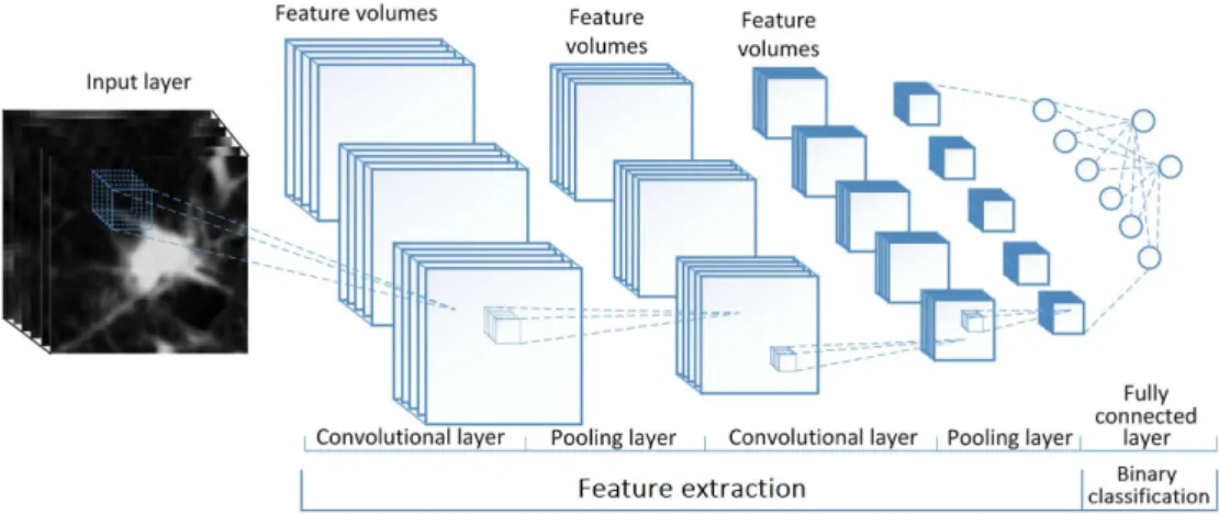
3-14 Addition of different projection views . . . 34 3-15 Blurry reconstruction through many views . . . 34 3-16 Corresponding sinogram . . . 34 3-17 Radio sensitivity of different tissues and organs [17] . . . 37 4-1 Artificial intelligence timeline, credits: Fractal Analytics . . . 39 4-2 Popularity of AI, ML & DL, credits: Sergey Feldman. . . 40 4-3 Moore’s law, credits: Our World in Data . . . 41 4-4 General ML model . . . 42 4-5 General supervised ML model . . . 44 4-6 Linear vs Logistic regression . . . 47 4-7 2D example of loss function landscape, credits: O’Reilly Media . . . 47 4-8 Linear regression . . . 49 4-9 Underfitting and overfitting [18] . . . 51 4-10 Error vs model complexity [19] . . . 52 4-11 Neuron, credits: @brgfx (Freepik) . . . 53 4-12 Perceptron . . . 54 4-13 Multilayer perceptron . . . 55 4-14 Activation functions . . . 60 4-15 Partially connected vs fully connected layers . . . 62 4-16 2D convolution . . . 63 4-17 Multiple convolutions . . . 64 4-18 Maxpooling . . . 64 4-19 Up-convolution, credit: Ashutosh Kumar . . . 65 4-20 Deep CNN for image classification [20] . . . 65 4-21 2D U-Net architecture [21] . . . 66 4-22 3D U-Net architecture [22] . . . 67 5-1 Ping An nodule detector . . . 72

6-1 Variation in segmentation between radiologists . . . 78 6-2 Spooky skeleton . . . 80 6-3 Segmentation of vascular tree . . . 81 6-4 Nodule size distribution . . . 81 6-5 Stochastic probability map of axial distribution of the nodules . . . 82 6-6 Example of original CT scan data . . . 83 6-7 Pre-processing of CT-scans . . . 84 6-8 Histgram thresholding . . . 85 6-9 Noisy scan examples . . . 86 6-10 Capture nodules in boxes [24] . . . 89 6-11 Overlapping extraction & reconstruction . . . 89 6-12 Translational augmentation in axial slice . . . 91 6-13 Nodule detector architecture [25] . . . 93 6-14 Residual 3D U-Net . . . 94 6-15 Dense 3D U-Net . . . 95 6-16 False positive reductor architecture [26] . . . 104 6-17 Malignancy and sphericity . . . 106 6-18 Distribution of malignancy . . . 107 7-1 Learning curve of reference model . . . 110 7-2 Example prediction . . . 111 7-3 Example of poor prediction . . . 111 7-4 Results of reference model . . . 112 7-5 Results of smaller boxes . . . 113 7-6 Difference in density . . . 114 7-7 Results when combining detectors . . . 115 7-8 Results of augmented detectors . . . 117 7-9 Results of different architectures . . . 118 7-10 Learning curve of initial false positive reducer . . . 120

7-13 Results for different γ values . . . 123 7-14 Results for different hard negative mining methods . . . 124 7-15 Results of rotations and flips . . . 125 7-16 Results for translation and combinations of augmentations . . . 127 7-17 Visualization example . . . 127 7-18 Affects of false positive reduction . . . 128 7-19 Learning curves of malignancy classifiers . . . 130 7-20 Large malignant tumor . . . 130 7-21 Outputs of the malignancy classifiers . . . 131 7-22 Output on top of scan and segmentations . . . 132 8-1 Example of poor prediction because of improper reassembly . . . 136 C-1 K-means clustering . . . 152 D-1 ROC curve . . . 153 D-2 Coin on small table . . . 154 D-3 Coin on larger table . . . 154 D-4 Difference in ROC curve . . . 155

2.1 Turnover time and surface area for different epithelial tissues [27][28][29] . . 13 2.2 surivival rates [30] . . . 18

AI

Artificial Intelligence ANN

Artificial Neural Network AUC

Area Under Curve DNA Deoxyribonucleic Acid FN False Negative FP False Positive TP True Positive TN True Negative CAD Computer-aided detection/diagnosis GPU

Graphics processing unit

MRI

Magnetic Resonance Imaging CT

Computer Tomography PCA

Principal component-analysis ReLU

Rectified linear units ROC

Receiver Operating Characteristic ROI

Region-of-interest TCIA

The Cancer Imaging Archive GBD

Burden of Disease COVID-19

Coronavirus disease SARS-CoV-2 3D

ML

Machine Learning DL

Deep Learning U-Net

U-shaped Neural Network LIDC-IDRI

Lung Image Database Consortium and Image Database Resource Initiative

NSCLC

non-small cell lung cancer SCLC

small cell lung cancer PET

positron emission tomography PFT

pulmonary function testing NMR

nuclear magnetic resonance RPM

rotations per minute PMT

Photo Multiplier Tube ICRP

International Commission on Radiological

NLP

natural language processing GD

Gradient Descent SGD

Stochastic Gradient Descent CNN

Convolutional Neural Network DNN

Deep Neural Network CADx

Computer Aided Diagnosis CADe

Computer Aided Detection FNIH

National Institutes of Health NCI

National Cancer Institute DICOM

Digital Imaging and COmmunications in Medicine

FPR

False Positive Reduction or False Positive Rate

TPR

Introduction

1.1

Problem Definition

Cancer is globally the second most common cause of death, only preceded by cardiovascular disease. This can be seen in figure 1-1. The data used for this plot originates from the Global Burden of Disease (GBD) database [31].

Figure 1-1: Most common causes of death [1]

Lung cancer specifically, is the most mortal type of cancer. Note that prevalence & mortality of different types of cancers can strongly depend on gender (e.g. breast & prostate cancer). The prevalence & mortality (respectively) of different cancers is visualized in figure 1-2.

Figure 1-2: The 20 most common causes of cancer deaths [2]

One reason for this high mortality rate is the fact that lungs are rather sensitive organs, which makes it difficult to diagnose and treat lung cancer without inflicting addition harm to the patient. Figure 1-1 also shows that other respiratory diseases, such as lung infections (e.g. COVID-19), account for the third most common cause of death globally. In general, pathologies of the lung are awfully deadly and as of today still form a major challenge for the medical field.

As an effort to reduce the burden of lung cancer and improve prognosis, lung cancer screen-ing has increasscreen-ingly become routine practice in high risk population groups. As a result of various anatomical aspects of the lung, one of the only practical methods for screening and diagnosis of lung cancer is the use of radiographs and CT scans. Unfortunately, lung tissue is some of the most radio-sensitive tissue in the human body. Therefore, lung cancer screening is generally performed through low-dose CT scans. As beam intensity is lowered to reduce the risk of induced radiopathologies, the signal-to-noise ratio and image quality is thus also significantly reduced. [32][33].

An important step in the diagnosis of lung cancer is the detection of pulmonary nodules (a.k.a. lung nodules, spots or lesions). A pulmonary nodule is a small round or oval-shaped growth in the lung. The relative size, shape of such nodule is strongly indicative of its chance to be cancerous. Lung nodules show large variations in shape, size and appearance.

Additionally, nodules often look similar to the neighbouring bronchi in a single slice of the CT scan. Lung nodules can generally be distinguished from these bronchi by looking at their three dimensional (3D) shape. This requires the radiologist to browse through consecu-tive slices of the CT scan and determining that the structure is indeed round/oval shaped [34].

All things considered, the consistent and accurate detection of lung nodules is a time-consuming and tedious task, resulting in a heavy workloads for radiologists.

For many years, computers have been used to try and develop Compute-Aided-Diagnosis (CAD) systems which may help reduce the work load of radiologists. The detection and diagnosis of lung nodule has specifically been one of the most challenging problems.

Supervised Machine Learning (ML) is a branch of Artificial Intelligence which learns by ex-ample from labeled training data. Deep Learning (DL) is a specific ML technique which has shown tremendous advances and impressive results in recent years. Deep Learning uses deep Artificial Neural Networks (ANNs) to construct a mathematical model which can compute the desired output for the given task. In this thesis a specific type of deep ANN is used, Convolutional Neural Networks (CNNs). What is truly revolutionary about these CNN as CAD systems is that the network learns by themselves which features of the CT scans are most important for the detection/diagnosis of the nodules. In classical methods such as ra-diomics on the other hand, the features were usually handcrafted based on the expertise of radiologists and had to be hard-coded by the engineers [35].

These new techniques have shown that computers have the potential to be faster, more accu-rate and have higher consistency than radiologists. For reference, a radiology specialization usually takes about 5 years after having completed 6 years of medical school. It is however important to note that this includes a wide variety of skills besides simply the detection and segmentation of lung nodules in CT scans. It takes a radiologist approximately 5-10 minutes to screen a CT scan for lung cancer [36]. The models developed for this thesis took in the order of several hours to be fully trained. Making predictions on a set of 853 scans took 3-5 days depending on the model, which also equated to about 5-10 minutes per scan.

However, the algorithms are in a sense faster than radiologists, as computers can run unin-terruptedly. Additionally, these time frames can be further improved with the use of better hardware and more computationally efficient coding.

Finally but perhaps most importantly, hiring radiologists is immensely costly. If part of the task is automated to speed up the process, it could reduce the hospital’s expenses significantly.

As mentioned before, radiologists have to browse through consecutive slices in order to esti-mate the 3D shape of a specific Region of Interest (ROI). This is one area where computers have a clear advantage over humans. Us human have two eyes, giving us some perception of depth. However, we do not have ”true” 3D vision as we are unable to look behind or inside 3D objects. Additionally, regular computer screens are inherently limited to 2D display. A computer on the other hand, could be trained to ”truly see in 3D”; computers can consider the CT scans as a 3D array rather than a series of 2D slices. This is the philosophy behind the use of 3D Convolutional Neural Network (CNNs), which is the type of Deep Learning architecture used in this thesis.

1.2

Objectives

As of today, computers are already rather fast and cheap. The huge challenge which machine learning engineers have to overcome is making sure that computers can achieve similar (or even better) accuracy and reliability as radiologists.

Although CAD systems have shown very impressive results in the detection of lung nodules, radiologists will most likely not be replaced by computer any time soon. This is partially because, although these systems might be very effective, a lot of people feel uncomfortable with leaving their diagnosis at the mercy of a computer [37]. The objective of this thesis is by no means the development of a system that can completely replace the task of a radiologist. Literature on lung nodule detection is often focused towards developing systems that mimic the behavior of (and even out-perform) radiologists.

In this thesis on the other hand, emphasis is put on aiding the radiologist in detection, seg-mentation and diagnosis (classification) of the nodules.

A 3D U-Net architecture was used in this thesis as nodule detector, which generates large amounts of false positives. This is usually counteracted by adding a secondary network which functions as False Positive Reducer. However, literature has shown that some of these false positives are actually true positives that were overlooked by the radiologists who helped cre-ated the training data [38]. Therefore, extreme false positive reduction is not desired in this thesis. The objective is to provide the radiologists with a probability map that highlights regions which the model ”suspects” of having a certain probability of being nodules. The analysis of the scan can be reduced to these suspicious regions, which should be further ex-amined by the radiologist. This should both save time as well as provide suggestive regions which the radiologist may not have thoroughly considered otherwise.

The objective of this thesis is thus, to use state-of-the-art Deep Learning techniques to de-velop a CAD system that automatically detects and segments lung nodules. In order to develop such system, large quantities of training data are required. The LIDC-IDRI dataset is used from The Cancer Imaging Archive [39]. This dataset which contains 1018 CT cases of 1012 different patients, annotated by four experienced radiologists.

.

1.3

Structure

Although the main topic of this thesis is situated in Computer Science, Chapter 2 and 3 are more oriented in biology and physics (respectively). This is because the author wanted this thesis to form a cohesion of the diverse study track followed (B.Sc. Engineering Physics, M.Sc. Biomedical Engineering), to which this work marks the end.

The reader is not assumed to have prior knowledge on any of the discussed topics. The majority of concepts are to built-up from the very basics, which results in this thesis being rather extensive. Chapters 2, 3, 4 & 5 can all be considered introductory as well as side information to get a broader view of the problem. If the reader is primarily interested in the research performed for this thesis, feel free to only consider chapters 6, 7 & 8.

• Chapter 2: Lung Nodules. Basic anatomy, biology and physiology of the lungs. Lung cancer, why it is so prevalent and deadly. Its diagnosis and treatment, clinical relevance and statistical observations.

• Chapter 3: Computed Tomography. How CT scans are made, the underlying physics followed by the design of a CT scanner and image reconstruction.

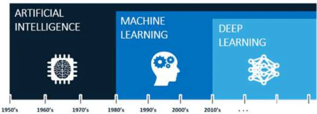
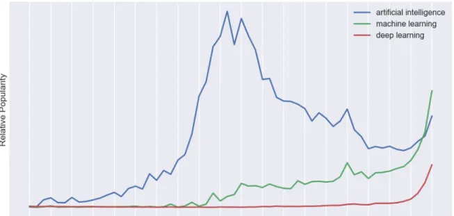
• Chapter 4: Deep Learning. How today’s cutting edge AI techniques are different from classical methods, where they come from and how they work.

• Chapter 5: Computer Aided Diagnosis. Describes the application of AI meth-ods in the medical field and discuss the state-of-the-art methmeth-ods that motivated the architectures used for this thesis.

• Chapter 6: Materials & Methods. Discusses the hardware, software and methods which were used for this thesis.

• Chapter 7: Results & Discussion. Discuss the results which were obtained with the use of these methods.

• Chapter 8: Conclusion. Final conclusions regarding this thesis, what are the main challenges and how can the results be improved in future work.

The appendices generally contains side information and parts that were deliberately left out of the main text of this thesis.

Lung Nodules

2.1

Respiration

Many organisms need oxygen to survive (aerobic organisms), this results from the basic chemical reactions that provide energy to cells, known as cellular respiration [40]. There is many possible biochemical reactions each with different reactants (carbohydrates, fats, proteins, . . . ) regulated by a complex variety enzymes. This is a rather complex field in of itself that will not be further discussed in detail.

However, to gain some general insight, consider the combustion (oxidation) reaction of glu-cose, which is also the preferred energy source in human cells, equation 7.1 [41].

C6H12O6+ 6 O2 → 6 CO2+ 6 H2O ∆G = −2880 kJ

mol (2.1)

This reaction is also exactly what many cells use to generate energy, 2880 kJ per glucose molecule to be exact, although a large portion of this is dissipated as heat. This energy is used to “charge up” (via e.g. Krebs cycle) tiny spring-like molecules known as ATP, which are present in the cells of every single living organism on earth, see figure 2-1.

The essential thing to notice in the above reaction is that oxygen (O2) is consumed and carbon dioxide (CO2) is formed. Thus, many organisms need a mechanism to extract oxygen from their surrounding environments as well a way to exhaust the generated carbon dioxide. Fish have gills to extract oxygen from oxygenated water, insects diffuse air though many tiny

Figure 2-1: Chemical potential energy stored in ATP [3]

openings in their body walls and us mammals have lungs that directly pump air in and out of our body from which the oxygen is extracted [42].

2.2

Lung Anatomy, Physiology and Pathology

The air comes in through the trachea which splits into the two main bronchi. From here, the number of bronchi exponentially increase by consecutive splitting up to approximately 2.105 bronchi which further split into alveolar tubes and eventually debouch into the alveoli. The alveoli are little sacs where the oxygen diffuses into the tiny capillaries while CO2diffuses out. The oxygen rich blood is carried towards the heart back into the blood circulation through the vascular tree in the lungs. [4].

Just like many organs in the human anatomy, the outer lining of the lungs is covered by epithelial cells. It is this epithelial layer that is responsible for the large majority of primary lung cancer cases [43].

Figure 2-3: Different types of cells in lung epithelium [5]

The epithelial lung tissue consists of a wide variety of epithelial cells, each with their own function. Ciliated cells have tiny hair-like structures at the top which help sweep debris, unwanted bacteria and mucus towards the throat where it can be swallowed or ejected via the mouth, this is known as the mucociliary escalator. Goblet cells play the major role in the secretion mucus. The main function of club cells is to protect the epithelium, this is accomplished by the secretion of different enzymes and small proteins. Neuroendocrine cells secrete hormones and thus have a signalling function in response to neuronal signals. Basal cells are mostly inactive and have the ability to replace any other cell type in response to injury. They are thought to be the stem cells as well as progenitor cells within the lung epithelium, this is still an active area of research. A final important category is immune cells such as dendritic cells and mast cells. These cells help protect the lungs from complications such as viral and bacterial infections. Previous lung complications such as infections also significantly increase the future risk of developing lung carcinoma [44]. Note that there are many more cell types which are not all discussed in this thesis [45].

2.3

Cancer

Cancer is a group of diseases characterized by two main properties: disproportionate cell expansion and metastasis. The general development process of cancer (in epithelial tissue) is visualized in figure 2-4. Metastasis is what makes cancer so deadly, if cancer was simply

an excessive expansion of cells, many cases could be cured through surgical resection. These cases are known as benign tumors which although closely related, are not considered to be cancer. Metastasis, the spreading to surround tissue, makes cancer difficult to treat and causes its high mortality rate.

Figure 2-4: Development process of cancer [6]

During cell division, under normal circumstances, the DNA of the healthy cell mother is duplicated in order to provide DNA to the daughter cell. It is during this duplication process that mutation is most likely to occur. Errors happen rather often during the DNA duplication process, luckily, the human body has mechanisms to resolve these mutations known as DNA repair. However, if these mutations are extremely unfortunate (or if the repair mechanism doesn’t function properly), the DNA can become unrepairably damages, which may result in significant changes in the behavior of a cell. This is the biological origin of cancerous cells.

The mutation of a healthy cell into a cancerous one generally results from many different individual errors in the DNA, therefore, this an almost continuous mutation process. As a result, the exact definition of a cancerous cell is rather ambiguous. In order for a cell to be ”truly cancerous”, the following properties are generally required: Rapid division, don’t show apoptosis, be invisible to the immune system, send out signals for resources (e.g. angiogenesis) [46][47].

Cancerous cells generally have very distinct histological features such as; irregular structure, large and even multiple nuclei, as can be seen in figure 2-5 [48]. The application of deep learning methods in microscopic biopsy images is also an active area of research [49].

Figure 2-5: Histology of cancer cells [7]

An average mature human body has somewhere between 20 − 40 trillion cells. Many millions of cell divisions occurs inside a single human body every second. The total amount of cells that are produced in a life-time is simply astronomical. Even if the chances of a perma-nent DNA error occurring during a cell division is extremely slim, the chance of it never occurring throughout an average lifetime is very improbable. In the (approximate) words of prof. Matthias Lutolf: ”The truth is that we all probably already have cancer, its just a matter of whether your body is able to keep it from escalating into detrimental symptoms” [8].

This is further supported by Peto’s paradox. Since different mammals are all made up of eukaryotic cells which are of similar size and structure, larger mammals are simply made up of more cells. Thus, one would statistically expect these large animals to be more prone to develop cancer. In reality the contrary is very much true, in fact, large mammals such as whales seem to be almost immune to developing terminal cancer. Large mammals may be filled with tumors, but since these tumors are relatively small compared to the organism as a whole, they may not be obstructive. The mammal may be much more likely to die from old age or other causes than from the cancer as it would take too long for the cancer to grow large enough to cause serious problems. Alternative reasons such as the concept of ”hyper tumors” may also play part in this phenomenon [50][51][52].

2.3.1

Cancer in Epithelial Tissues

Part of the function of the outer epithelial cell lining of organs is to protect it and other organs from the surrounding environment: the epithelial cells in our skin form the primary barrier to protect us from the outside environment, the epithelial cells in our gut protect our inner organs from the harsh intestinal environment and many microbes that make up the intestinal flora. Similarly, the epithelial cells in the lungs form a barrier that protects our insides from any harmful matter that may come with the air we breathe in. As a result of epithelial cells being in contact to the harsh outside environment, they frequently have to be renewed. Thus, they have a high rate of cell divisions (short turnover-time), see table 2.1. Note that the turnover time strongly depends on which part of the lungs is considered. The turnover time of the trachea for example, is usually more than a month [53].

Risk of mutations is also significantly influenced by the presence of contaminants. Some of the biggest influencers that increase the risk of lung cancer are: smoking, radioactive (radon) gas, asbestos air pollution [54].

As a result of the branching discussed before, lungs have a large effective surface area and thus, these epithelial cells are rather numerous, see table 2.1.

Conclusion: The epithelial cells in lungs divide frequently and are numerous, therefore there is a high amount of cell division per unit time. As cells become cancerous through DNA errors, and DNA errors usually occur during cell division, The probability of an epithelial tissue developing cancerous cells is approximately linear to the cell division rate of that tissue (when ignoring other influencing factor). Therefore (lung) epithelial tissue, which has a high effective surface area and short renewal time is statistically more likely to develop cancer. This roughly quantified by equation 2.2 and table 2.1.

Skin Lungs Intestine Effective Area 1.5-2.2 m_² 50-75 m_² 25-40 m_² Renewal time 2-6 weeks 1-2 weeks 5-7 days

Table 2.1: Turnover time and surface area for different epithelial tissues [27][28][29] According to this statistical philosophy, lungs and the intestine should have a similar prob-ability of developing cancer, while for the skin this should be significantly lower. These findings actually agree surprisingly well with the statistics discussed in previous chapter. Figure 1-2 showed that bowel and lung cancer have similar prevalence, while skin cancer has a significantly lower prevalence.

2.3.2

Immortal Cells

Stem cells are defined as (at least partially) undifferentiated cells that have the ability to renew themselves allowing them to (in theory) divide and live forever. Unfortunately, it is statistically impossible for this to work endlessly and every cell does have to die at some point. However, this mechanism is what has allows humans reach lifespans of more than a hundred years.

Every human starts off as a single (stem) cell. This cell divides, resulting in a group of cells which eventually forms what is known as a blastocyst. The inner cell mass of the blastocyst are known as ”embryonic stem cells”. These stem cells will go on the form every single possible cell type of the mature human body [8].

A full grown human primarily consists of differentiated cells that have a specific function (e.g. blood cells, skin cells, neurons, etc..). However, as discussed in previous section, many differentiated cells eventually die off and must be replaced. Generally, this is achieved through a complex hierarchy of stem cells and progenitor cells. Every tissue has its own complex system and as of today this is still very much an active area of research. An example of such hierarchical system (small intestine) is displayed in figure 2-6 (for lungs: not well known).

Figure 2-6: Cell hierarchy of the small intestine [8]

The stem cells generally divide rarely since they function as safeguard of the DNA sequence. In a sense, stem cells are the like the primal cells that remained in that undifferentiated state of the embryonic stem cells that we all started from. Stem cells are the fundamental reservoir that is essential in maintaining our genetic information. The progenitor cells on the other hand, function as the workhorse of the hierarchical system, they divide frequently and differentiate into the functional cells. The functional cells generally don’t divide, they serve their function for as long as they live, after which they are (usually) cleared from the body. Although many progenitor cells also show some self-renewal characteristics, eventually they do die and need to be replenished, which requires a stem cell to divide. The characteristic that sets stem cells apart is that they can (in theory) endlessly renew themselves and keep dividing indefinitely. Whenever a cell divides, the DNA has to be replicated, this process is visualized in figure 2-7.

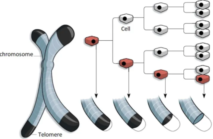
This machinery of enzymes walks across the DNA strand and duplicates it. However, when it reaches the very end of the DNA (which is folded into a chromosome), it is unable to properly replicate this final part. In order to prevent DNA from being lost in this process, the end of chromosomes are what is known as telomere. Telomeres are regions of repetitive, non-coding DNA that thus acts as a buffer to protect the chromosomes. However, due to the above described problem, the telomeres shorten with every cell division. Eventually the telomeres are depleted, this is detected by the cell as DNA damage and generally results in cell death (senescence or apoptosis). This is known as the Hayflick limit and if visualized in figure 2-8 [55].

Figure 2-8: Degradation of telomeres with cell divisions, credits: WSJ research

Progenitor cells as well as other cells that divide frequently (including certain stem cells) avoid this by expressing an enzyme known as telomerase, which restores the telomeres at the end of the chromosomes. The great majority of cells in the adult human body do not express any telomerase. Cancer cells also abundantly express telomerase [56][57].

Conclusion: Cancer cells have quiet a few things in common with stem cells and progenitor cells, which allows them to divide indefinitely. In the human body, there can be only two types of ”immortal” cells; stem cells and cancer cells.

2.4

Lung Cancer

2.4.1

Diagnosis

Some common symptoms of lung cancer include: coughing (with blood), shortness of breath, weight loss, weakness, fever, clubbing of the fingernails, chest pain, bone pain, superior vena cava obstruction, or difficulty swallowing [58].

A common first investigative step when showing signs of lung cancer is a chest radiograph. However, many diseases can give similar appearance to lung cancer on a radiograph such as; metastatic cancer, hamartomas, and infectious granulomas caused by tuberculosis, histoplas-mosis or coccidioidomycosis. These difficulties in differential diagnosis are much less prevalent in CT imaging. Therefore, CT imaging is generally used for pulmonary nodule surveillance in clinical practice [59].

There is different types of lung cancer, depending on which type of cell the cancerous mu-tation originates from. The type of lung cancer can be identified based upon histological examinations. This is an important step in the lung cancer diagnosis process as the type of lung cancer has big influence on the treatment as well as the life expectancy of the patient. Additionally, it helps distinguish primary lung cancer from metastatic cancer [60].

Based upon prognosis, there are two main groups of lung cancer; small cell lung cancer (SCLC) non-small cell lung cancer (NSCLC). NSLCC is further sub-divided into; adenocar-cinoma, squamous-cell caradenocar-cinoma, and large-cell carcinoma. The relative prevalence of each of these types as well as their relative statistical relation to smoking is conveniently visualized in figure 2-9 [9].

Figure 2-9: Relative prevalence of main lung cancer types and relation to smoking [9]

Adenocarcinoma originate from glandular cell types such as goblet cells of the epithelial lung tissue, which secrete mucus as discussed before. It is the most common type of cancer, especially for non-smokers as can also be seen in figure 2-9 [61].

Squamous cell carcinoma originate from Squamous cells which are a type of epithelial cells.0 that has not yet been discussed, they are specialized in the absorption and/or transport of substances. Within the lungs, they are primarily found in the alveoli and play a crucial role in the diffusion process of respiration.

Large cell carcinoma can originate from a range of different epithelial cell types, it is in essence a ”diagnosis of exclusion” that classifies the cancer as being part of the NSCLC group but not Adenocarcinoma or Squamous cell carcinoma. As a result, this cancer type can appear in any part of the lung and has many sub-types.

Small cell lung cancer (SCLC), although not yet fully understood, is thought to originate from neuroendocrine cells. It is significantly more mortal than the NSCLC group, the 5-year survival rate upon diagnosis is approximately 4 times lower. This results from the fact that SCLC spreads much faster than NSCLC due to its rapid cell division. It is thus highly ma-lignant and in most cases the cancer has already spread to various other parts of the body upon initial diagnosis [62].

2.4.2

Survival Rates

In the the table below, the stochastic 5-year relative survival rates are found for the two main groups separately as well as all cases combined [30].

Lung Cancer: 5-year relative survival

NSCLC SCLC Combined

Localized 61% 27% 54%

Regional 35% 16% 31%

Distant 6% 3% 5%

All Combined 24% 6% 20% Table 2.2: surivival rates [30]

The survival rates is strongly dependent on the developmental stage of the cancer at the point of diagnosis. In clinical practice, a rather more complex subdivision of stages is used which also varies depending on the type of lung cancer. However, the subdivision: Localized, Regional, Distant can generally be made for any type of lung cancer. Localized means that the cancer has not spread beyond its place of origin. Regional means the cancer has spread to surrounding tissue. Distant means the cancer has entered the general blood stream and has spread to distal parts of the body.

The final general conclusion which is important in the framework of this thesis is that sur-vival chances of lung cancer can be significantly improve if the cancer is diagnosed at an early stage. This is why lung cancer screening using low-doses CT scans is increasingly become routine practice, which is also the origin of the data used in this thesis. However, this causes a high work load for radiologists as screening CT scans for lung cancer is a rather tedious process.

2.4.3

Treatment

The treatment of lung cancer is undeniably a complex decision process that depends on the exact type of cancer, stage, clinical indications and even the specific institution where the patient is treated. However, there are some general guidelines that should be followed in any lung cancer manifestation.

Most importantly, smoking is by far the major risk factor for lung cancer. For people who smoke, quitting smoking is by far the most effective way of preventing lung cancer. Anyone who is diagnosed with any type of lung cancer at any stage should immediately and indefi-nitely stop smoking.

Numerous studies have also shown that regular exercise promotes stem cell proliferation and migration to injured tissue which can significantly improve healing. Therefore, exercise and other lifestyle improvements such as a healthy, non-excessive diet is always advised [63].

More specific treatments include: surgical resection, chemotherapy, targeted therapy, hor-mone therapy, radiation therapy and others. These may be used in combination with one another to assure an optimal treatment.

Surgical Resection

Generally, surgical resection is the preferred treatment for many cancer/tumor types. How-ever, a single surgical resection can only cure the cancer if it is in a localized stage. Addition-ally, surgical resection can only be applied to tissues that are not crucial for the patients sur-vival. Surgical resection is primarily applied for NSCLC. Because of the rapid growth/spread of SCLC, it can rarely be cured through surgical resection. However, it may still be applied as it can slow down the spread of the SCLC.

Whether or not surgical resection is applicable can be determined through a series of exami-nations, depending on the case this may include; CT, PET-CT, blood tests, (needle) biopsy, endoscopy (mediastinoscopy, thoracoscopy), pulmonary function testing (PFT), ... [59][64].