Insights for the third Global Environment Outlook from related global scenario analyses. Working paper for GEO-3

Hele tekst

(1)research for man and environment. RIJKSINSTITUUT VOOR VOLKSGEZONDHEID EN MILIEU NATIONAL INSTITUTE OF PUBLIC HEALTH AND THE ENVIRONMENT. RIVM report 402001017 Insights for the third Global Environment Outlook from related global scenario analyses Working paper for GEO-3 J.A. Bakkes, C.G.M. Klein Goldewijk, J.R.Meijer, D.S. Rothman (ICIS), H.J.M. de Vries, J.W. van Woerden September 2000 Global Dynamics and Sustainable Development Programme GLOBO REPORT SERIES NO. 28. With contributions by J. Alcamo (CSER), B.J. ten Brink, G. van Drecht, H.B.M. Hilderink (NIDI), P. Martens (ICIS), S. Nijhof (ICIS) CSER: Center for Environmental Systems Research, University of Kassel NIDI: Netherlands Interdisciplinairy Demographic Institute, The Hague ICIS: International Centre for Integrative Studies, Maastricht. This investigation has been performed by order and for the account of The Netherlands’ Ministry of Public Housing, Spatial Planning and the Environment, and the United Nations Environment Programme (UNEP), within the framework of RIVM project 402001, contributions to the Global Environment Outlook.. RIVM, P.O. Box 1, 3720 BA Bilthoven, telephone: 31 - 30 - 274 91 11; telefax: 31 - 30 - 274 2971.

(2) page 2 of 67. RIVM report 402001017. Acknowledgements This working paper has been compiled under great pressure of time. Fortunately, quite a few people were prepared to contribute information in one form or another. They include: Johannes Bollen, Lex Bouwman, Michel den Elzen, Eric Kreileman, Rob Swart, Detlef van Vuuren (all RIVM); Paul Raskin and Alyssa Holt (SEI); Nebojša Nakicenovic (IIASA); Thomas Henrichs and Thomas Rörsch (CSER).. National Institute of Public Health and the Environment P.O. Box 1 3720 BA Bilthoven, The Netherlands Telephone: 31 30 274 3112 (direct) Fax: 31 30 274 4435 E-mail: Jan.Bakkes@rivm.nl HTTP://www.rivm.nl. Cover design: Martin Middelburg, Studio RIVM.

(3) RIVM report 402001017. page 3 of 67. Contents 1.. Introduction and Guide to the User. 7. 2.. Lessons for GEO-3 from the SRES Process. 9. 3.. Sample Insights on Impacts. 13. 3.1. POPULATION. 16. 3.2. ENERGY. 20. 3.3. EMISSIONS TO AIR. 24. 3.4. LAND. 28. 3.5. CLIMATE. 36. 3.6. WATER. 40. 3.7. BIODIVERSITY. 44. 3.8. HUMAN IMPACTS. 48. 3.9. ECONOMIC ACTIVITY. 52. 4.. Suggestions for questions to focus GEO-3 scenario analysis. 55. 5.. Conclusion. 57. APPENDIX I: Sectoral Storylines APPENDIX II: Economic Growth Rates APPENDIX III: Suggestions for Summary Indicators.

(4) page 4 of 67. RIVM report 402001017.

(5) RIVM report 402001017. page 5 of 67. Summary This report relates to the ongoing development of scenarios for the third Global Environment Outlook (GEO-3) of UNEP. It illustrates the scale and type of environmental impacts that GEO-3 needs to consider. It does so by quantifying impacts using existing, recent studies whose scenarios come closest to the current tentative global storylines for GEO-3 (see Raskin, Preliminary Frameworks). With a view to GEO-3’s envisaged role as input for the Rio+10 Earth Summit in 2002, this report suggests a focus for the GEO-3 scenario analysis on the potential for co-benefits between development and environment policies. Moreover, a set of three summary indicators is proposed, to reflect the impact of the scenarios on three domains of sustainable development. The quantification in the report addresses issues such as: the demographic transition and changing dependency ratios of populations; water shortages; changes in the yield of crops; risk of land degradation; and the loss of terrestrial biodiversity. Special attention is given to regional differentiation and to material that will help to estimate how vulnerability of humans and ecosystems changes in the scenarios. We present this as an invitation and a challenge to the regional centers to produce regional scenarios with the ultimate goal being the production of regionally specific, globally consistent, alternative scenarios for GEO-3..

(6) page 6 of 67. RIVM report 402001017. Samenvatting Dit rapport maakt deel uit van de voorbereiding van de derde Global Environment Outlook van UNEP. Het illustreert schaal en soort van de milieu-effecten die GEO in beeld zou moeten brengen. De effecten worden gekwantificeerd door materiaal dat is ontleend aan recente studies over min of meer vergelijkbare scenarios. Omdat het de bedoeling is dat GEO-3 de milieu-onderbouwing levert voor de Rio+10 milieutop in 2002 wordt in dit wekdocument de suggestie gedaan om de analyse voor GEO-3 te richten op de mogelijkheden voor synergie tussen milieubeleid en ontwikkelingsbeleid. Verder worden drie samenvattende indicatoren voorgesteld. De kwantificering in dit werkdocument heeft betrekking op onderwerpen als demografische transitie en afhankelijkheidratio in de bevolking; watertekorten; veranderingen in gewasopbrengst; de kans op landdegradatie; en de achteruitgang van biodiversiteit. Speciale aandacht is besteed aan regionale verschillen en aan informatie die van belang is voor het schatten veranderingen in kwetsbaarheid..

(7) RIVM report 402001017. 1.. page 7 of 67. Introduction and Guide to the User. The production of the outlook chapter for GEO-3 strongly depends on the timely development of regional and global scenarios. This report has been prepared as a resource for the participants of the September Working Meeting in Cambridge to assist in this effort. We focus here on quantifying the impacts of scenarios such as those that will be developed for GEO-3. The current report is meant to be an illustrative exercise and does not represent the final version of the global scenarios. This can be accomplished only after further discussion on the regional implications of the GEO-3 storylines and the development of the regional scenarios. For the reasons given above and time pressures, no new calculations have been done for this report. Rather, we have brought together illustrations from recent studies, selecting those scenarios that best match the broad scenario descriptions that emerged from the meeting of the core scenario group in Boston this past July. Obviously, there is not a perfect match between the eventual GEO-3 scenarios, the scenarios from which we have drawn for this report, and the illustrative data at region level from earlier exercises. We also acknowledge that the time pressure under which this report has been prepared has resulted in obvious gaps that should be discussed during this meeting. However, we feel that the material presented here is useful for identifying the key issues on which the GEO-3 scenario analysis needs to focus. The purpose of the material presented here is to help in the following: • Identifying key issues and trends that need to be taken into account in GEO-3 scenario work - within regions, between regions, and globally. • Identifying impacts that warrant in-depth analysis for GEO-3, in view of the scale of change, regional differences and vulnerability issues. • Identifying additional information sources, such as region-oriented models, that need to be included for the GEO-3 scenario analysis to adequately reflect regional and global issues in light of the policy questions GEO-3 seeks to address. The remainder of this report is structured as follows. Section II identifies key lessons for GEO-3 scenario development from the recent IPCC SRES exercise. Section III presents the key results of our illustrative quantification of two of the GEO-3 scenarios. Section IV provides suggestions for key questions on which to focus the GEO-3 scenario analysis. Section V concludes and points the way to the further development of the GEO-3 regional and global scenarios..


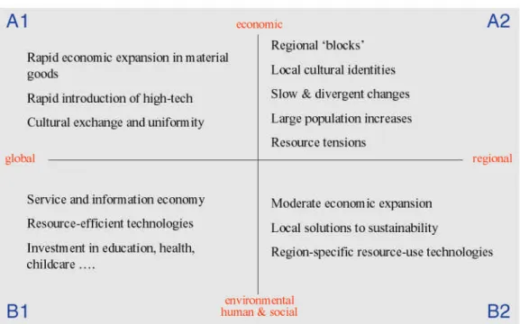
(9) RIVM report 402001017. 2.. page 9 of 67. Lessons for GEO-3 from the SRES Process. There have been a number of scenario exercises in recent years from which GEO can benefit. Perhaps the most significant of these is the IPCC’s Special Report on Emission Scenarios. Here we present a summary of some lessons from this process. Combining Qualitative Storylines with Quantitative Models After a review of existing scenarios and analyzing their main characteristics and driving forces, the SRES team formulated a set of narrative storylines to describe alternative futures. This drew upon the experience of the Global Scenarios Group. The storylines were distinguished across two dimensions: the relative emphasis on global vs. regional development and on economic growth vs. environmental protection (see Figure II.1). At first there was some resistance to the use of narrative storylines, but over time their value began to be appreciated. Whereas the quantitative model results lent consistency to the scenarios, the storylines allowed for the creation of much richer stories. Also, the models used were better suited for describing the more globalized futures. Looking solely at the quantitative outputs, e.g. the higher populations and lower per capita incomes, the more regionalized futures could be interpreted as less ‘desirable’. However, the rich narrative of the storylines makes it clear that this is not the case. 1 Allowing for Broad Input: The Multi-Model Process and the Open Process The SRES process included six modelling teams – 2 American, 2 European, and 2 Asian and associated models. 2 There were advantages to this effort, e.g. allowing a clear distinction to be made between uncertainties represented by different assumptions concerning driving forces and those due to model representation of particular processes. It is not clear, though, that this outweighed the disadvantages. The most important of these was the lack of consistency in regional representation. The final results were presented at the level of just four aggregate regions, hiding more regionalized detail that could have been provided by any of the individual modelling teams. This information would have been quite valuable for policy; it may still be possible to recover and use. Another part of the SRES process relates to this - the Open Process. This provided access to the SRES process, including detailed information on the storylines and preliminary versions of the quantitative scenarios. It also allowed for comments and submissions of additional existing scenarios and new scenarios based on the SRES storylines to be included in the scenario database. 3. 1. There is a related note on the naming of the scenarios. Names were proposed for the four scenario families, but these were problematic. They were found to either be too one-dimensional or open to too many possible and conflicting interpretations. 2 Although all of the modelling teams were from OECD countries, the full writing team had a broader regional representation. 3 In all, “more than 34,000 accesses to the SRES web site were registered by April 1999 from some 3,000 unique hosts” (SRES report, p.354)..

(10) page 10 of 67. RIVM report 402001017. Acknowledging the Infeasibility of Prediction and Multiple Baselines One of the most important criteria the SRES team set was the creation of a set of baseline scenarios, none of which was to be considered “best guess” or “business-as-usual”. 4 A clear consensus has emerged that for complex environmental and socio-economic systems “the long-rang future cannot be extrapolated or predicted” (Raskin, Preliminary Frameworks). There was no disagreement within the writing team and the creation of multiple baselines has resulted in a richer and more credible product. In the review process, there were some concerns expressed about the implications of having to deal with multiple baselines. This is a reflection of a more general tension between scientific credibility and policy making, which may also surface in the GEO process. The Specification of Scenarios and Resulting Limitations The purpose of the SRES scenarios were to provide “input for determining future climate patterns”, “the basis for the assessment of vulnerability, possible adverse impacts and adaptation strategies and policies to climate change”, and “the basis for the assessment of possible mitigation strategies and policies designed to avoid climate change” (SRES report, p.23). Their intended use is for “future IPCC assessments and by wider scientific and policymaking communities for analyzing the effects of future GHG emissions and for developing mitigation and adaptation measures and policies” (SRES report, p.23). Importantly, their terms of reference specified that they “exclude additional initiatives and policies specifically designed to reduce climate change” (SRES report, p.25). These preconditions limited the SRES team in two ways. First, the futures explored could not consider explicit climate policies. There were debates concerning the distinction between climate and non-climate policies, particularly for the ‘B’ scenario families. Regardless of the exact distinction, it is clear that this restriction did prevent the writing team from considering a certain range of policy actions and, therefore, the futures that would follow from these. The second way in which the specification was limiting is in the focus on the issue of climate change. The IPCC, in its forthcoming Third Assessment Report, places the issue of climate change within the broader perspective of development, equity, and sustainability. This was also the case in the early stages of the SRES process but as the work proceeded, particularly in the quantification of the scenarios, much of this richness was lost. Only those elements of a broader set of issues that would be desired in a more holistic economic-environment-social scenario that are directly related to the climate issue were included in the final versions. This is reflected, in part, in the lack of a broad set of economic, environmental, and social indicators. Resources SRES work lasted three years and has involved a writing team of about 50 people, spread over the globe. A conservative estimate puts the effort of the writing team at approximately 20 person-years of scientific staff. In addition, much effort was devoted to compiling a database of preceding scenario work, to expert and government review and to coordination. In all, this seems beyond the current scale of resources for GEO-3 scenario preparation, making re-use of existing analyses all the more desirable.. 4. The need to be explicit concerning this matter was, in part, in response to the use of the IS92 scenarios. Despite numerous recommendations that the full set of scenarios be used, the IS92a scenario rapidly established itself as the reference, from which the others were considered deviations..

(11) RIVM report 402001017. page 11 of 67. Summary There are a number of lessons for the GEO-3 process that can be drawn from the above observations. A few of these are listed below: • • • • •. combine storylines with quantitative elaboration of the scenarios; make use of participatory processes, including a formal “Open Process” on the internet to allow for contributions from a wide range of researchers and interested parties; use multiple scenarios to illustrate fundamentally different yet plausible futures; make use of published and unpublished material available from the SRES process and other recent scenario exercises (e.g. the GSG work and the World Water Vision regional scenarios) wherever possible; and include a manageable yet broad set of economic, environmental, and social indicators reflecting GEO’s broad and integrated character.. Figure 2.1: The four different domains depicted by the SRES narratives.


(13) RIVM report 402001017. 3.. page 13 of 67. Sample Insights on Impacts. Introduction This section presents the results of a sample scenario exercise at the global level. The two scenarios considered are the Conventional Development and Policy Reform scenarios. As shown in Table III.1, each of these are comparable in character to existing scenarios developed by the IPCC, the Global Scenarios Group, the World Water Vision, and the World Business Council for Sustainable Development. Initial storylines for each scenario are presented in the preliminary framework document (Raskin, 2000). Due to the short time frame between the GEO-3 meetings in Boston and Cambridge, the quantitative interpretations presented in the figures and tables have been taken from existing work, mostly on quantifying the related SRES scenarios, specifically A1 for Conventional Development and B1 for Policy Reform. Thus, although the results reflect those we would expect for the GEO-3 scenarios, it is important to remember that this is only an illustrative exercise. In interpreting the SRES storylines, two dimensions were used to differentiate the scenarios: the extent of convergence between regions and the extent of environmental awareness. The former, represented by the global – regional axis in Figure II.1, addresses the degree of globalization as expressed in, for example, convergence of market-based mechanisms and instruments, trade liberalization, size of interregional capital flows and rate of dissemination of technical innovations. The latter, represented by the economic – environmental, human & social axis in Figure II.1, addresses the degree of social and environmental awareness as expressed in widespread support for, for example, solidarity between the rich and the poor, ‘green’ lifestyles and technologies and community-oriented experiments towards a more sustainable future. The process of convergence between regions generally is modelled by assuming a ‘leader’, towards which parameter assumptions in all other regions move. It is not necessary that the same region act as leader for all parameters. Given the initial differences between regions, the degree of convergence is determined either by a target date by which convergence is complete or a specific parameter, usually GDP/capita, in which case the parameter assumptions converge as the regional values for the specific parameter converge. The parameter assumptions in the lead region can change over time, creating the effect of the other regions chasing a moving target. Different scenarios can be distinguished in several ways: convergence can occur for different sets of parameters; different regions can serve as the leader for specific parameters; dates of convergence can differ; and the parameter assumptions for the lead region(s) can evolve differently. The quantification of the scenarios presented here has been achieved using a set of complementary and partially linked models: the WorldScan model of CPB, Netherlands [macro-economy]; the PHOENIX model (developed at RIVM) [demography and population health]; the IMAGE model of RIVM [environmental impacts]; and the WaterGap model of CSER, Germany [water stress]. The ‘translation’ of the qualitative assumptions about the scenarios into quantitative assumptions for the models can be divided into several clusters:.

(14) page 14 of 67. • • • • •. RIVM report 402001017. population; economic activity, including total growth, sectoral growth, and trade (with specific assumptions on food and energy related trade); life-style, including total consumption and preferences; technology, in general and more specifically in the energy and agricultural sectors; and resource base.. Both the Conventional Development and Policy Reform scenarios assume that the present trends of globalization and liberalization continue such that regional differences decline over time. Thus, they share many common assumptions, most importantly regional population growth. The primary differences between the scenarios are driven by their positions along the second axis noted above – environmental awareness. Table III.2 provides a summary of the key differences in assumptions between the scenarios. These reflect the overall assumption of a society that places primary emphasis on economic growth in the Conventional Development scenario vs. environmentally benign and equitable development in the Policy Reform scenario. More detail on the sectoral implications of these scenarios is presented in Appendix I of this report. Although we do not present results here, it is useful to recognize that quantification of the Fortress World and Great Transition scenarios at the global level is a more complicated task in that there are fewer rules of the game in terms of consistency across regions. Many different paths are possible for individual regions, as long as they remain ‘compatible’ at the global level. Thus, the development of the global scenarios for these two variants will be very dependent upon the results of the regional activities. The remainder of this section presents a comparison of how the differing assumptions for the Conventional Development and Policy Reform scenarios translate into different impacts. Table 3.1 Scenarios Compared GSG. SRES. Conventional Worlds Reference Policy Reform. A1 B1. Barbarization Breakdown Fortress world. A2. Great Transitions Eco-communalism New sustainability paradigm. WBCSD. FROG! GEOpolity. GEO-3. Conventional Development Policy Reform. Fortress World. B2. Source: Raskin, Preliminary Frameworks. Jazz. Great Transition.

(15) RIVM report 402001017. page 15 of 67. Table 3.2: Key Differences between Assumptions for Conventional Development and Policy Reform Scenarios (as approximated by SRES A1 and B1) Population Urbanization maximum percentage lower in Policy Reform Economic Activity Total growth lower in Policy Reform Energy taxes converge to EU levels in Policy Reform, to US levels in Conventional Development Energy prices higher premium factors added to fossil fuels, primarily coal, in Policy Reform Trade trade in agricultural products lower in Policy Reform Payback period required longer in Policy Reform for investments in energy efficiency Energy subsidies reduced and eventually eliminated in Policy Reform Life-Style Food preferences meat consumption in lead region lower in Policy Reform Wood demand demand in lead region lower in Policy Reform Other demands demand for energy intensive commodities in lead region lower in Policy Reform Technology Total factor productivity lower growth in energy-intensive sectors in Policy Reform Fertilizer use maximum level lower in Policy Reform Animal productivity, slower convergence in Policy Reform extraction rates, fraction of animal feed from crops, and feed requirements Pollutant emission factors where currently lower than in lead region, rate of convergence from land use and slower in Policy Reform; also regional abatement factors applied agriculture to most emission factors in Policy Reform Learning curves faster for renewables in Policy Reform; slower for nuclear in Policy Reform Demonstration projects Included for renewables in Policy Reform Energy efficiency Ultimate potential higher in Policy Reform Resource Base Agricultural land Limited in Policy Reform to avoid deforestation.

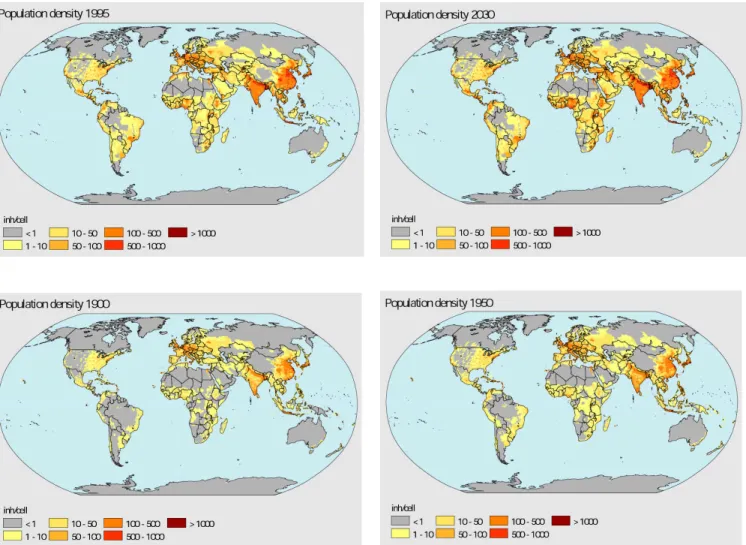
(16) page 16 of 67. 3.1. POPULATION. Figure 3.1.1Population density. One cell = 0.5 x 0.5 degree (approximately 50 x 50 km at the equator). RIVM report 402001017.

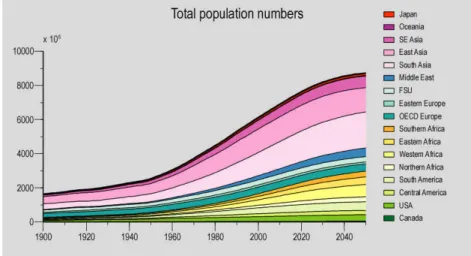
(17) RIVM report 402001017. Figure 3.1.2: Total population. Figure 3.1.3: Dependency ratio. Figure 3.1.4: Total fertility rate. page 17 of 67.

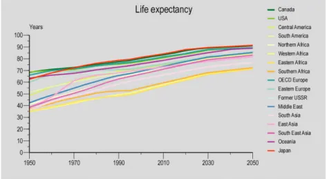
(18) page 18 of 67. Figure 3.1.5: Life expectancy at birth. RIVM report 402001017.

(19) RIVM report 402001017. page 19 of 67. What can be seen? Both scenarios use the same demographic assumptions so they are not distinguished in these charts. The global population is expected to reach just under 9 billion by 2050, at which point little or no further growth is expected. The fastest growth between now and 2050 occurs in South Asia and the African regions. The population density increases in these regions reflect this growth, with the worldwide changes in population density hinting at the increased urbanization, even in regions with less overall growth. The dependency ratios – the ratio of population under 15 and over 65 versus the population between 15 and 65 – rise considerably in the regions with little or no overall population growth, reflecting the increasing numbers of elderly in their populations. For the faster growing regions this falls early in the century, levelling off and starting to increase at midcentury. How does this connect to the storylines? These patterns reflect the changes assumed concerning fertility rates and life expectancy based upon the stage at which different regions are in the demographic transition. It is assumed that all regions will complete the fertility component of the demographic transition, i.e. a decline in fertility rates to around replacement level, by 2030. Some differences do remain between regions with respect to the ultimate level of fertility, with some regions below and others above replacement. Similarly, assumptions on the mortality component of the demographic transition are reflected in increases in life expectancy in all regions. These increases are much smaller in regions with the longest current life expectancies, but significant differences still remain at mid-century. Overall, these changes are such that global population will see a decline beyond the time period of this scenario. For the currently low-income regions, increasing dependency ratios will pin down important resources, thereby increasing the regions’ vulnerability environmental change. See for example the projection for East Asia. Source. Website. RIVM adapted from IIASA input to SRES Historical data from the HYDE Database (RIVM), projections derived with PHOENIX model http://www.rivm.nl/env/int/hyde and www.rivm.nl/image/phoenix.

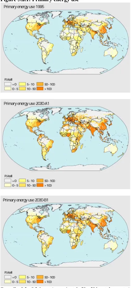
(20) page 20 of 67. 3.2. ENERGY. Figure 3.2.1: Primary energy use. One cell = 0.5 x 0.5 degree (approximately 50 x 50 km at the equator). RIVM report 402001017.

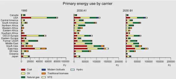
(21) RIVM report 402001017. Figure 3.2.2: Primary energy use per carrier. Unit: PJ/year. Figure 3.2.3: Final energy use by sector. Unit: PJ/year. Figure 3.2.4: Primary energy intensity. Unit: MJ energy use per $ GDP (ppp basis). page 21 of 67.

(22) page 22 of 67. RIVM report 402001017. What can be seen? In both scenarios, primary and final energy use increases in all regions, with the greatest increases in the currently least industrialized regions (Latin American, Africa, and Asia). In the A1-world, the increases are larger, resulting in an almost tripling of global primary and final energy consumption. In the B1-world, primary and final energy consumption ‘only’ doubles. The share of natural gas is expected to grow substantially, with large reductions in the share of coal, particularly in the B1-world, and slight reductions in the share of oil. The use of renewable resources and modern biofuels will grow modestly, with somewhat larger growth in the B1-world. The share of energy provided by traditional biomass falls, with greater declines in the A1-world. The household share of final energy use falls, whereas the transportation share rises in both scenarios. The key difference between the two scenarios is in the share of industrial energy use, which rises in the A1-world and falls in the B1-world. As expected, these patterns differ between regions. Primary energy intensity falls in all regions in both scenarios, with the exceptions of South America and Northern Africa in the A1-world. The decline is most striking in the Former USSR and the other African regions. The decrease is somewhat stronger in the B1-world than in the A1-world. How does this connect to the storylines? The patterns of energy use are primarily driven by the assumptions related to economic growth and technology. In both scenarios all regions will eventually converge to similar levels of energy use as their GDP/capita figures converge. The higher rates of economic growth in the A1-world are the primary reason for the greater amount of primary energy use. The greater potential for reductions in energy intensity in the B1-world also contributes to this difference as well as to the lower realized values of energy intensity in this scenario. The preference for cleaner fuels expressed in the form of increased premiums and demonstration programs assumed in the B1-world, explain the differences in fuel mix. Source Website. TIMER (part of IMAGE2.2), RIVM. http://www.rivm.nl/image.

(23) RIVM report 402001017. page 23 of 67.

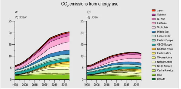
(24) page 24 of 67. 3.3. EMISSIONS TO AIR. Figure 3.3.1: Carbon dioxide emissions from energy use. RIVM report 402001017.

(25) RIVM report 402001017. page 25 of 67. What can be seen? Global emissions of carbon dioxide from energy use increase in the early years of both scenarios due to growth in population and activities. Over time, however, the emissions decrease in the B1-world, with the A1-world having significantly higher emissions. We can also see the growing share of emissions from the currently less developed regions, notable South Asia and the African regions. How does this connect to the storylines? The overall increase in emissions in both scenarios is partially a result of increased population, but more due to the rapid rates of growth in activities. Developments in technology somewhat offset these increases. The differences between scenarios mainly reflect the faster growth in activities in the A1-world. They are also influenced by the reduced energy intensity, greater emissions controls, cleaner fuel mix, and reduced demand for animal products in the B1-world. A similar pattern could be shown for emissions of other greenhouse gases such as methane and nitrous oxide: an increase during the early years of both scenarios, with over time significantly larger emissions in the A1-world. In the B1-world, the release of methane eventually starts to decrease as well. Source. RIVM, IMAGE 2.2.

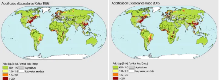
(26) page 26 of 67. RIVM report 402001017. Figure 3.3.3: Acidification: Exceedance of Critical Loads. Figure 3.3.4: Eutrophication by nitrogen: Exceedance of Critical Loads.

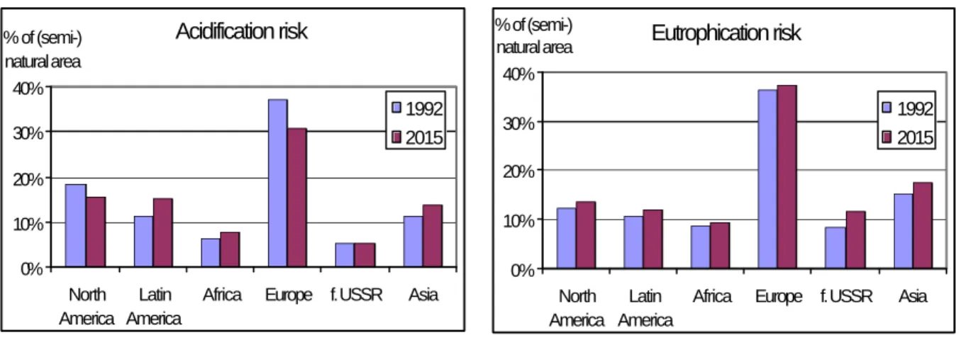
(27) RIVM report 402001017. page 27 of 67. Figure 3.3.5: Acidification and Eutrophication: exeedance of critical loads, by region % of (semi-) natural area 40%. % of (semi-) natural area 40%. Acidification risk. 1992 2015. 30%. 1992 2015. 30%. 20%. 20%. 10%. 10%. 0%. Eutrophication risk. 0% North Latin America America. Africa. Europe f. USSR. Asia. North Latin America America. Africa. Europe f. USSR. Asia. What can be seen? The projections show the human influence on regional element cycles (in this case: sulphur and nitrogen cycles) spreading further outside the traditional industrialized regions. In highincome regions the acidification pressure on ecosystems will on average decrease. But in currently low-income regions the acidifying emissions will strongly increase. Nitrogeneutrophication pressure on natural ecosystems will increase everywhere, except in Europe. How does this connect to the storylines? These results are drawn from a scenario assuming the implementation of Current Reduction Plans. For acidification, although energy use and mobility are projected to rise in this scenario, control measures are assumed to be continued and enhanced, especially in the currently highincome nations. The increase in eutrophication pressure by nitrogen compounds corresponds to an increase in emissions from all major sources, including thermal power generation, transport and the use of nitrogen fertilizers in agriculture. Most of these are expected to increase further. The use of nitrogen fertilizers is assumed to have reached a maximum in most of the currently highincome regions but may well increase in tropical agriculture. Conditions at the subregional scale (soil, ecosystem, climate, and other natural circumstances) determine how vulnerable ecosystems are to deposition of acidifying and eutrophicating substances. Therefore, even ecosystems in sub-regions with relatively small emissions such as West and Central Africa may see a significant increase in pressures, in particular in an A1-world. Source Publication. Website. RIVM, IMAGE 2.1 UNEP/RIVM (1999). A.F. Bouwman and D.P. van Vuuren Global assessment of acidification and eutrofication of natural ecosystems. UNEP/DEIA&EW/TR.99-6 and RIVM 402001012 : http://www.rivm.nl/env/int/geo/.

(28) page 28 of 67. 3.4. LAND. Figure 3.4.1: Land use. RIVM report 402001017.

(29) RIVM report 402001017. page 29 of 67. Figure 3.4.2: Domesticated Land. What can been seen ? Globally, domesticated land continues to expand at the expense of natural area, but there are significant differences between regions. At the extremes the share of domesticated land falls by nearly half in Canada, whereas it increases by nearly than two and a half times in Western Africa. The general pattern is for increases in domesticated land in the currently low-income world and decreases in the currently high-income. Japan is a notable exception. Both scenarios show just the beginning of the development of noticeable amounts of land used for the production of biofuels. How does this connect to the storylines? On balance, the differences between the scenarios are small up to 2030 even though the underlying dynamics are not the same. The overall increase in domesticate land is slightly larger in the A1-world (a 16% increase) versus the B1-world (a 14% increase), with a very slight shift of balance in favour of pasture and fodder over food in the A1-world relative to the B1-world. The land use changes are primarily driven by population growth, changes in consumption and changes in technology (primarily in the agricultural sector). Secondary (often regionspecific) effects are due to urbanization, land degradation, trade developments, and the climate. The emergence of modern biofuels is a sign of what may be ahead: by 2050, the area used especially for the production of biomass for energy production is estimated at 19% or 24% of the global crop area. The subtle difference between the A1 and B1-worlds are primarily due to the lesser emphasis given to the consumption of meat and diary products in the latter. Source Website. IMAGE 2.1.2. Historical data from the HYDE Database, RIVM http://www.rivm.nl/image / http://www.rivm.nl/env/int/hyde.

(30) page 30 of 67. Figure 3.4.3: Change in potential yields of various crops. RIVM report 402001017.

(31) RIVM report 402001017. page 31 of 67. What can be seen? These figures show a complicated story in terms of changes in crop yields over the next century. Both increases and decreases in yield are seen for different crops and regions. A closer inspection does reveal some very general patterns, however. Areas that show benefits for most crops include the north central US, southern Canada, Eastern Europe and the former USSR, the southern peninsula of India, and northeast China (with the important exception of rice). Western Europe, particularly in the Mediterranean region, northeastern India, the interior of China, and Australia consistently show decreases. All of these changes are more subtle in the B1-world, reflecting the smaller changes in climate in this scenario. How does this connect to the storylines? Crop yields are a function of climatic factors, inputs such as fertilizer, cropping intensity, and agricultural management. Not all crops can be grown in all regions. As illustrated here, climate changes differ by region, leading to increasing yields in some areas and decreasing yields in others. The impacts of other factors are not shown, but it can be assumed that improvements in agricultural management lead to increasing yields over time in all regions, with the rate of improvement differing between regions and between scenarios. Also, the greater fertilizer use in the A1-world should also result in slightly greater increases in yields in this scenario. In both scenarios more detailed analyses would show changes over time as the climate keeps changing, passing from more beneficial climates to less beneficial for certain crops and regions. Source Website. IMAGE 2.1.2, RIVM http://www.rivm.nl/image.

(32) page 32 of 67. RIVM report 402001017. Figure 3.4.4 Vulnerability to water-induced soil degradation, 1995. Figure 3.4.5 Vulnerability to water-induced soil degradation, 2030 A1. Figure 3.4.6 Vulnerability to water-induced soil degradation, 2030 B1.

(33) RIVM report 402001017. page 33 of 67. Figure 3.4.7 Vulnerability to water-induced soil degradation, by region. What can be seen? The amount of land at risk from erosion increases in both scenarios, with a slightly greater increase in the A1-world. In both scenarios, the greatest increases occur in Africa other than North Africa and in Asia. In the United States, although there is a decrease in total area subject to erosion risk, a greater percentage shifts to the high-risk category. In some regions such as Canada and Oceania, overall decreases in vulnerability are seen. How does this connect to the storylines? The risk to water induced soil degradation reflects land use and natural conditions (soil properties, slope, but also climate) and land management 5 . Thus, changes in vulnerability are primarily driven by climate change, agricultural demand and technology. The B1-world, which sees slightly less land shifted to domestication, thus should be expected to have a slightly smaller erosion vulnerability. Whether land degradation actually occurs is not only determined by the risk but also by the effectiveness of soil conservation management. The likelihood of effective soil management seems larger in an A1 than in a B1-world.. 5. The water erosion vulnerability index expresses the vulnerability of the land under a specific form of land use. The vulnerability is composed of the land’s so-called susceptibility and the type of land use (i.e. the land use pressure index). The susceptibility is defined as the vulnerability of the bare soil (i.e. terrain erodibility), based on the specific soil and terrain conditions (soil properties, slope, slope length) and climate (i.e. rainfall erosivity). In the map and graph the index is presented for all classes or categories between 0 (no water erosion risk in case of natural vegetation) to 1.0 (highest risk) with steps of 0.05. Based on validation of the model results against the GLASOD water erosion assessment of Oldeman et al. (1990), actual water erosion risks occur at index values greater than 0.15. High water erosion risks are associated with index values of 0.30 and beyond..

(34) page 34 of 67. RIVM report 402001017. As severe degradation of agricultural land usually leads to a demand for land in order to make up for production capacity lost, and as new land conversion may well increase degradation risks again if pushed to vulnerable areas, land degradation and land conversion can easily reinforce each other, in the absence of effective soil management. Therefore, it is significant that the largest increases in degradation risk are shown for regions where the risks are already largest, and where agricultural land use is expected to grow fastest. Source Publication. IMAGE 2.2, RIVM Hootsmans RM, AF Bouwman, R Leemans, GJJ Kreileman and GJ van den Born (2000, in prep.). Modelling land degradation in IMAGE 2. RIVM (report no. 481508009), Bilthoven.. Further reading (Technical background and ground-thruthing related the modelling of land degradation, ISRIC/UNEP/RIVM): • Batjes, NH (1996). A Qualitative Assessment of Water Erosion Risk using 1:5 M SOTER Data. An application for Northern Argentina, South-East Brazil and Uruguay. Report 96/04, International Soil Reference and Information Centre, Wageningen. • Batjes, NH (1996). Global Assessment of Land Vulnerability to Water Erosion on a ½ by ½ 0 Grid. Report 96/08, International Soil Reference and Information Centre, Wageningen. • Mantel, S and Engelen, VWP van (1997). The Impact of Land Degradation on Food Productivity. Case studies of Uruguay, Argentina and Kenya. Report 97/01. International Soil Reference and Information Centre, Wageningen.


(36) page 36 of 67. 3.5. CLIMATE. Figure 3.5.1: Temperature change. RIVM report 402001017.

(37) RIVM report 402001017. page 37 of 67. Figure 3.5.2: Change in mean annual temperature. Figure 3.5.3: Sea-level rise. What can be seen? Over the next half century, the global mean temperature is expected to rise by more than 1.2°C in the A1-world versus slightly over 0.8°C in the B1-world. (This is on top of a 0.40.7°C since 1900.) By 2050, the A1 scenario has set into motion a further increase of approximately 0.2°C every ten years. There are significant differences between regions, with a general pattern of larger warming at higher latitudes and in the interior of continents. Associated with the rising temperatures is an increase of sea level on the order of 20 cm, once.

(38) page 38 of 67. RIVM report 402001017. again with a larger increase seen in the A1 scenario. However, the differences between the regions are much smaller than between the scenarios. How does this connect to the storylines? Changes in climate are driven by changes in atmospheric concentrations of radiatively active gases and large-scale changes in land use, both of which are driven by population growth, activity increase, and technological changes. Both warming caused by greenhouse gas emissions and cooling caused by sulphur oxides have been taken into account in these estimates. The greater warming in the A1-world is primarily related to the increased energy use in this scenario. The greater warming at higher latitudes and in the interior of continents are related to physical processes in the climate system. Source RIVM/IMAGE (maps: version 2.1, charts: version 2.2) Further reading, overview: Hughes, L., 2000. Biological consequences of global warming: Is the signal already apparent? Trends in Ecology and Evolution, 15: 56-61..


(40) page 40 of 67. 3.6. WATER. Figure 3.6.1 Change of Water Stress. RIVM report 402001017.

(41) RIVM report 402001017. page 41 of 67. Figure 3.6.2 Change of Water Stress, by Region. What can be seen? In the Business as Usual (BAU) scenario, the great contrast in the water situation between industrialized and developing countries is likely to continue. Between 1995 and 2025 the number of people living in areas with ‘severe water stress’ grows from about 2.1 to 4.0 thousand million. The increase is especially significant in Southern Africa, Western Africa and South Asia. The Values and Lifestyles (VAL) scenario produces a very different picture. Here, outside of parts of South America, sub-Saharan Africa, and central Asia, water stress decreases throughout the world. With growing populations, however, especially in Africa, this still results in an increase of people living in areas with ‘severe water stress’ to 2600 million. How does this connect to the storylines? The results for the water stress maps are drawn from two scenarios developed for the World Water Vision – BAU and VAL. The former is roughly consistent with the Conventional Development storyline of GEO-3. The latter could be considered consistent with the Policy Reform storyline, but may fit better with the Great Transition storyline. The BAU scenario assumes that water withdrawals in most industrialized countries decrease and therefore the pressure on water resources also decreases. Meanwhile, withdrawals grow in most developing countries and increase the pressure on their water resources. In river basins under severe water stress there will be strong competition for scarce water resources between households, industry and agriculture. In the VAL scenario, every developing country achieves a minimum domestic water use adequate to meet basic needs (40 l per capita per day) . Second, water withdrawals drop very sharply in industrialized countries compared to business-as-usual. Finally, water withdrawals in developing countries stop growing even though their economies and material well-being grows tremendously. But some trends may.

(42) page 42 of 67. RIVM report 402001017. continue. For example, total withdrawals continue to grow substantially in many parts of Africa, Latin America and Asia because of increasing population, and because of economic growth and aspirations that come with it. This, however, does not lead to a large increase in the areas under severe water stress in Africa and Latin America because the growth occurs mostly in water-rich areas. In these regions the problem may not be water shortages, but instead the need to rapidly expand water infrastructure to accommodate increasing water demands. The estimates assume that a river basin is under ‘severe water stress’ if the ratio of annual withdrawals over average annual availability is greater than 0.4. Sensitivity analyses have shown that this is fairly robust. But the effect of severe water stress will be different in different countries. In industrialized countries water is often treated before it is sent on to downstream users, and industry recycles its water supply fairly intensively. For these and other reasons industrialized countries can often heavily utilize their water resources without negative consequences. By comparison, wastewater in developing countries is usually not treated, and industries do not recycle their water supplies as often. Hence, intensive use of water here can lead to the rapid degradation of water quality and quantity for downstream users, and frequent and persistent water emergencies.. Source Publication. Center for Environmental Systems Research, University of Kassel Joseph Alcamo, Thomas Henrichs and Thomas Rösch (2000). World Water in 2025. Global modeling and scenario analysis for the World Water Commission on Water for the 21st Century. Center for Environmental Systems Research, University of Kassel Website http://www.usf.uni-kassel.de Further reading Water Futures in the World Water Vision; and GEO-1 and technical background reports.

(43) RIVM report 402001017. page 43 of 67. Figure 3.6.3: Local water shortages and urbanization. What can be seen? The increasing number of people at risk from water stress gets an extra boost from urbanization in low-income regions. That is, if urban water supply systems are not drastically improved. In Africa the increase in urban population at risk from water stress is almost three times the increase in total population. In Latin America and South Asia the urban population at risk from water stress increases between 100 and 150%. How does this connect to the storylines? 6 Urbanization concentrates people, but not the available water. If an agglomeration is situated within a drainage basin that on average is at risk from water stress, probabilities are that the water stress will be amplified in the urban area. This is not only because most of the people live there anyway, but also because urban water infrastructure in many situations has no greater reach than 50 to 100 km. Thus, it cannot bring together the available water to the degree necessary. In practice, the severity of the problem depends on technical and economic possibilities to cope with it (by storing or importing water, or by using deep groundwater). This once more points to the fast growing urban population in low-income regions as the most vulnerable. Source Publication. RIVM RIVM (2000) Nationale Milieuverkenning 5 (Fifth national environmental outlook). National institute of Public Health and the Environment (RIVM), Bilthoven, The Netherlands Further reading Drecht G van en JM Knoop (2000, in prep.) Water Stress Assessment and Forecast at the global Scale; Development of a computer program for simulation of water demand and water availability for global scale analysis of water stress, WARiBaS 1.07. RIVM (report no. 402001016), Bilthoven.. 6. The estimates shown are aggregates of worldwide calculations for areas of 0,5 x 0,5 degree (approximately 50x50 km at the equator). For areas this small, it is assumed that severe water stress occurs if the ratio of annual withdrawal over annual average availability in is 0.5, as opposed to 0.4 for evaluation at the drainaige basin level..

(44) page 44 of 67. 3.7. BIODIVERSITY. Figure 3.7.1: Ecological Capital Index. RIVM report 402001017.

(45) RIVM report 402001017. page 45 of 67. Figure 3.7.2: Ecological Capital Index, by region. What can be seen? The Ecological Capital Index7 decreases in almost all regions in both the A1 and B1-worlds. This change is significantly smaller in the B1-world, reflecting the greater attention paid to environmental issues. Globally, this crude measure of terrestrial biodiversity decreases between 1990 and 2030 by 12 percent-points in the A1-world and 8 percent-points in the B1world. These global changes hide large regional differences, though. Japan and South Asia see their values fall by one-third and Africa and the Middle East see declines of nearly a quarter in the A1-world. Little or no change is seen in Latin America in both scenarios. The index is currently lowest in parts of Europe and Asia.. How does this connect to the storylines? In Africa land use change dominates the picture and in Asia and West-Asia increases in pressures. In North-America and Oceanea, a significant agricultural area will be being taken out of production during the first decades of the scenarios. The natural quality of this area will be modest, but that is not captured by the crude measure used here. In the global average the agricultural area being taken out of production masks the large loss of current nature, especially in the tropics and subtropics. This makes the global picture too rosy. Moreover, as the maps show, there is quite a lot of variation within regions in both scenarios. The changes are most dramatic in tropical areas of Africa and Asia, that is, in ecosystems with very rich biodiversity. By the middle of the century, the remaining ‘true’ natural areas, i.e. those not. 7. The Ecological Capital Index (ECI) tries to capture both the quantity and quality of natural areas. The quantity is more or less a direct measure of the the percentage of area that is natural. The quality is a reflection of species abundance. Given the lack of detailed data in most regions, ecosystem quality can also be approximated using pressure information, based upon calibrations within regions where both are available. As pressure increases, it is assumed that ecosystem quality will decrease. The key pressure factors or proxies of pressure used here are: climate change, population density, density of energy use, and logging..

(46) page 46 of 67. RIVM report 402001017. represented by reclaimed agricultural land, are mostly found in less habitable or remote areas such as deserts, mountains and boreal forest. Source Publication. RIVM [On the index:] UNEP (1997). Recommendations for a core set of indicators of biological diversity. Convention on Biological Diversity, UNEP/CBD/SBSTTA/5/12, and inf. 13, Montreal. United Nations Environment Programme, Nairobi, Kenya. Website http://www.rivm.nl/env/int/geo Further reading GEO-1 and technical background reports. [On the index] Ten Brink (2000). Biodiversity indicators for the OECD Environmental Outlook and Strategy. A feasibility study. With a contribution from the World Conservation Monitoring Centre. RIVM report 402001014. National Institute of Public Health and the Environment, Bilthoven, The Netherlands WCMC (2000). Natural capital indicators for OECD countries. World Conservation Monitoring Centre - World Conservation Press, Cambridge, United Kingdom [On biodiversity scenarios] Sala et al. (2000). Global Biodiversity Scenarios for the Year 2100. Science, 10 March 2000, Volume 287, pp. 1770-1774..


(48) page 48 of 67. 3.8. RIVM report 402001017. HUMAN IMPACTS. Figure 3.8.1: Human Development Index (HDI). What can be seen? The general pattern is for regional HDI values to converge over time as a result of income growth and increased life expectancy. The most rapid growth over the next half century is seen in Northern Africa and Southeast Asia. However, the rank order of the regions by the middle of the century will not be very different from the present. The three southern African regions and South Asia continue to lag behind. For reasons described below, the regional HDI values differ only slightly between the A1 and B1-worlds over this time period and are, therefore, not shown separately. How does this connect to the storylines? The HDI is computed as a function of life expectancy, educational attainment, and income growth. The A1 and B1-worlds, as presented here, do not differ in the former two categories, although both categories do rise in both scenarios. Thus, the different convergence rates reflect only disparities in GDP growth. These also do not differ significantly between the scenarios; thus, the lack of distinction between the two scenarios in terms of HDI. One has to keep in mind that the HDI has been developed to rank countries, not to assess and comprehend the extent of development. In particular, the use of average levels for income conceals important disparities within a country or region. Nevertheless, the change in HDI can serve as a starting point to describe the development of a country or region qualitatively in order to subsequently focus on key regional aspects of the scenario..

(49) RIVM report 402001017. Source. Publication. Website Further reading. page 49 of 67. RIVM and NIDI (Netherlands Interdisciplinary Demographic Institute). Estimations have been carried out using the PHOENIX model. Hilderink (2000). World Population in Transition. An Integrated Regional Modelling Framework. Thela Thesis, Amsterdam, The Netherlands www.rivm.nl/image/phoenix.html UNDP (1998) Human development report, United Nations Development Programme, New York..

(50) page 50 of 67. Figure 3.8.2 Potential Malaria Transmission. Unit: Continuous Months of Potential Malaria Transmission. Figure 3.8.3 Vulnerability to Malaria. Index scale: see inset below map. RIVM report 402001017.

(51) RIVM report 402001017. page 51 of 67. What can be seen? The general pattern is a slight expansion of the areas susceptible to malaria transmission at the current northern climate limits, with some increased intensity in terms of continuous months of transmission (e.g. parts of South East Asia and the US along the Gulf of Mexico). The areas already highly susceptible to malaria transmission, i.e. in Africa and Latin America see little change in months of transmission. Most areas benefit from a reduced level of vulnerability as their average incomes rise. How does this connect to the storylines? Climate change determines the changes in area where malaria can be transmitted 8 . As shown in section III.5, at higher latitudes larger temperature increases are expected. Vulnerability further reflects the ability of societies to provide protection against the disease, via environmental and/or health controls. On balance, the assumed large growth in GDP/capita in both scenarios makes vulnerability for the currently low-income regions decrease.. Source Publication. 8. ICIS Nijhof S. and Martens P. (2000) Climate Change Impacts on Vector Borne Diseases. Dutch National Research Program on Global Air Pollution and Climate Change (NRP) (in prep.). Potential malaria transmission is estimated as a function of climatic parameters, specifically mean monthly temperature and precipitation. These are estimated from an understanding of the biology of the mosquitoes that carry the parasite, which transmits the disease. Without adequate rainfall or temperature, the mosquito cannot survive. The relationship between GDP/capita, continuous months of transmission, and the vulnerability index have been calibrated against expert opinion of vulnerability by country..

(52) page 52 of 67. 3.9. ECONOMIC ACTIVITY. Figure 3.9.1: GDP per capita. Figure 3.9.2: Contribution to GDP by Sector. RIVM report 402001017.

(53) RIVM report 402001017. page 53 of 67. What can be seen? The most rapid growth is assumed in the currently lowest income regions, particularly the African regions, South and Southeast Asia. High growth rates are also expected for the countries of Eastern Europe and the Former USSR as they recover from the economic downturns experienced in the 1990s. It is clear, though, that parity, in terms of GDP per capita across regions, is not achieved in either scenario. The B1-world shows a more rapid shift to services from industry, even though the regional growth rates are on average lower. How does this connect to the storylines? The growth rates in GDP/capita are input assumptions as derived in the SRES process. Economic growth in terms of GDP per capita is projected to be robust in both the A1 and B1worlds. 9 As would be expected, the growth rates in the A1 world are higher for most regions. The overall result is an increase in economic activity between 2000 and 2030 of more than 140% in the A1-world and slightly over 110% in the B1-world. The strong growth in both scenarios and the differences between regions follow from the assumptions of healthy economies and rapid convergence. The lower growth rates in the B1-world reflect the assumption of a lesser emphasis on economic growth and more emphasis on social and environmental policies. The changes in contribution to GDP by sector reflect historic patterns and the general theories of structural change and economic development. This amounts to a general pattern of shrinking shares for agriculture and growing shares for services as countries develop, with industry initially increasing in contribution and then decreasing. The largest changes are seen in the declines in agriculture in the most rapidly growing regions. The greater emphasis on environmental quality in the B1-scenario accelerates the transition away from industry and towards services, which is generally a ‘cleaner’ sector.. Source. 9. RIVM, IMAGE 2.2, interpretation of SRES Scenarios, using Worldscan (of the CPB Bureau of Economic Policy Analysis). See Appendix for further discussion of the growth rates in the A1 and B1 scenarios..


(55) RIVM report 402001017. page 55 of 67. 4. Suggestions for questions to focus GEO-3 scenario analysis Increasing vulnerability to environmental change has been suggested as the overall theme for GEO-3. Building on separate preparatory work 10 on human vulnerability, the scenario analysis must therefore focus on issues related to both exposure to pressures and coping capacity. This implies the inclusion of both environmental and societal factors in the scenarios. The key areas of vulnerability are inherently different between regions; thus the choice of which areas to focus on will be left to the regional outlook teams. In view of GEO-3’s role in preparing for the 2002 Earth Summit (‘Rio+10’) another policy theme for the Outlook Chapter of GEO-3 is to focus on the potential for co-benefits between development [e.g. industrial and agricultural renewal, investing in education or diversification of the economy; and subsidy reform], and environmental [e.g. urban and long range air pollution; forests; land-related issues, and climate] policies. GEO-2000 hinted at this in very broad terms. The potential for co-benefits, or ancillary benefits as it is called in terms of climate policy, is a key issue in the climate debate. It is also becoming an important notion in at least EU environmental policy. In the outlook chapter of GEO-3, policies that warrant analyzing for their co-benefits potential will probably also change the vulnerability of people and/or ecosystems. GEO-3 is in a unique position to take the broad perspective that is required in order to analyze the potential for co-benefits. Although the scenarios will maintain an environmental window on sustainable development, GEO-3 provides a more holistic and integrated vision than has been presented, for example, by the IPCC in their SRES scenarios. That is, GEO-3 considers development and environmental policies with respect not only to their relation to climate issues, but to the much broader concerns of society as a whole. The GEO-3 process is also better placed to account for regional differences, the scenarios being developed with “mutual conditioning” between their global and regional specifications.. 10. See Draft paper: An Assessment of Human Vulnerability due to Environmental Changes [Work in Progress].


(57) RIVM report 402001017. 5.. page 57 of 67. Conclusion. In this report, we have presented a detailed and region-specific analysis of the GEO-3 storylines as input for the production of outlook chapter of the final report. The results of this exercise reveal: • • •. existing spatially explicit projections allow at least a start to be made with quantifying changes in vulnerability as a function of the GEO-3 scenarios; there exist large disparities in environmental impacts and vulnerability between and within regions; and there can be expected very fast increases in problem areas such as population at risk from severe water stress, and loss of terrestrial biodiversity. These preliminary results underline the need for the spatially explicit evaluation of the GEO3 scenarios. This is necessary before any final conclusions can be drawn. These preliminary quantifications of the GEO-3 global storylines have been produced from recent scenario-based studies, such as the IPCC’s SRES and the World Commission on Water for the 21st Century’s World Water Vision. Much of the material in this report is taken from the SRES A1 and B1 scenarios, as these come closest to the GEO-3 global storylines. Unpublished documents from the various groups that have contributed to SRES, as well as published and unpublished material from other studies, can also be rich resources for the elaboration of the GEO-3 scenarios. This is especially important with regard to the regional specificity that is the goal of GEO-3. In combination with the theme of changing vulnerability, we suggest that co-benefits between development and environmental and climate policies can provide a useful policy focus for the outlook chapter. In particular, this enhances the orientation of the chapter towards the goals for the Rio+10 process. We have also noted a few issues that need to be considered in the preparation of the GEO-3 scenarios from the existing storylines. The SRES A1 and B1 scenarios are strongly oriented towards convergence between presently low-income and high-income regions with respect to per capita levels of GDP. This results in growth rates of per capita income that lie far outside the range of similar studies; at the same time there remains a wide gap between the currently low-income and high income regions. Secondly, the two GEO-3 storylines we have not considered here – Fortress World and Great Transition – present particular difficulties for quantification due to their wider scope for regional variation. Third, the time and resources available for this effort are quite limited in comparison to other studies, such as the IPCC’s SRES process. Finally, including a formal “Open Process” on the internet during a specific period of time can allow for contributions to GEO-3 scenario work from a wider range of researchers and interested parties. These present challenges to both the regional centers and the core scenario group. However, they should not deter us from achieving our the ultimate goal of the production of a set of regionally specific, globally consistent, alternative scenarios for GEO-3..


(59) RIVM report 402001017. page 59 of 67. APPENDIX I. Sectoral Storylines In this appendix, we present further detail on the assumptions behind the A1 and B1 SRES scenarios. These focus on three sectors: mobility, transport and communications; manufacturing; and land & food. This material is drawn from previously unpublished material that was prepared during the SRES process and represents an example of the information that is available. A1 Mobility, transport and communications: The trend towards declining transport costs, both for passenger and freight, will continue as a result of improved logistics and other technical innovations. Passenger transport will be dominated by the private car; freight transport by trucks and [underground] pipelines. The number and intensity of vehicle use will go up. The shift in transport modes towards more air travel will continue, and the average trip will be faster and further. In the developed regions, saturation will occur at levels determined by population density, traffic congestion and the like. In regions with low population density, saturation levels for car ownership will move towards the present US-levels. In other regions governments cope with congestion problems by giving widespread support for road infrastructure investments. Public transport will be limited in most regions because political will and public funding are insufficient; it will be confined to, for instance, high-speed trains for medium range and bus/tram for urban regions. Tourism will become an ever more important source of income for parts of Asia, Africa and Latin America. The expansion of communications technology allows a further convergence in lifestyles and in technical and managerial values and skills. Electronic transfer of data and knowledge will further enhance the globalization of the financial service sector and trade. The highly volatile capital flows may result in economic and political instabilities, but these are effectively countered by global institutions. In the developed regions with high-density and aging populations, tele-working and teleshopping will help to low down the growth in physical flows of people and goods en services at the local level. Media such as TV and internet, on the other hand, induce a further growth in long-distance travelling and the marketing of exotic goods. These factors also strengthen the trend towards even more knowledge-intensive economic activities in these regions. Some less developed regions will see an accelerated penetration of mobile phones – thus avoiding heavy infrastructure investments. This induces a faster transition towards a service- and information-oriented economy. Manufacturing: The use of basic materials will saturate towards the present values in the OECD-regions. A global, competitive business environment will induce a high rate of technical innovation, which will generally be less resource-intensive. Worldwide production of basic materials such as steel and plastics will increasingly take place in coastal regions long major transport routes, and in connection with coals and oil trade. Both financial and physical flows will increasingly become part of global business. Multinational corporations increasingly dominate research, development and production and compete on the basis of flexibility and global cost minimization. Robotization accelerates the rise in capital-labour ratios; in some regions this is a response to labour shortages, in other regions it reinforces the trend towards a dual economy. Nanotechnology and recycling cause.

(60) page 60 of 67. RIVM report 402001017. major reductions in materials-intensity. Car manufacturers will be increasingly producing for a global market with rapid diffusion in innovations, low transportation costs and high rates of return on private capital. Land/food: This future will be characterized by a further expansion of the industrial food system, with increasingly western-style meat-rich diet and ready-made meals, frozen and concentrated foods, use of microwave etc. Subsistence agriculture gives way to commercial farming for domestic consumption and export, which is increasingly dominated by high-tech intensive methods using more irrigation and artificial fertilizer, pesticides etc. Use of these inputs will become much more productive thanks to the application of precision agriculture and biotechnology. Technological innovations will be disseminated rapidly throughout the world. Management schemes will become economically optimized with help of satellite observations, computerized seeding and feeding, irrigation schemes etc. Biotechnology will pay an ever more important role, in all parts of the food chain. Financial flows will be large and managed by the multinational agro-industry complex. Food will widely be traded based on comparative advantages. The developed regions (North America, Europe) will keep the lead in furthering high-tech capital-intensive mixed farming, introducing controlled greenhouses, hydroponics, bioengineering etc. As productivity rises further, land will become less and less of a constraint and large areas become available for other use (reforestation, recreation, biofuel plantations). Some will keep importing animal food (soja, corn); most will export cereals. Export of seeds and of plants will increasingly become part of the agro-business. China and India will push for a second ‘green revolution with loans from international institutions. Regions such as Africa and Latin America may specialize in tropical products for export while importing an increasing fraction of their local food needs and inputs (fertilizer, machinery). They – and also regions like India and China – will import genetically modified, patented seeds. Fuelwood is rapidly replaced by commercial fuels.. B1 Mobility, transport and communications: To solve environmental and congestion problems, there is an active policy to invest in infrastructure (subways in large cities, bicycling lanes, clean electrically driven buses etc.). Intercity traffic is increasingly by fast trains, with excellent local transport systems (including car rental). New and efficient ways for freight transport such as underground pipelines and rail systems are gradually introduced. Air traffic is for the largest part international. Although the private car remains the most important passenger transport option, both ownership and mileage saturate in most regions at much lower levels than present-day U.S. levels. Average fuel efficiency improves with a factor 5 to 10; electric and hybrid ([m]ethanol-based) cars make up an ever larger share of the market as they are appreciated for their convenience and low noise and pollution levels. The over-all economic activity related to transport (car manufacturing, gasoline, roads etc.) is growing at lower rates than in Business as Usual scenarios – after all, the value added per unit of time when bicycling is small. This is one of the explanations of the relatively lower rate of economic growth in this scenario. The rapid expansion of telecommunication technology gives the less developed regions important leapfrogging opportunities. For instance, sparsely populated regions in Africa and Latin America jump into GSM and satellite systems, bypassing material-intensive.

(61) RIVM report 402001017. page 61 of 67. infrastructure. Communications technology allows the introduction of effective family planning programs. Government and community-based programs for education, medical aid and resource management are rapidly becoming available for rural populations, which in combination with energy supply from local and renewable resources enhances the earning opportunities and in turn slows down the growth of megacities. Global communications networks have to comply with certain standards which regulate, for instance, the amount and nature of commercial advertising. Manufacturing: The trends towards lower energy and material-intensity is reinforced by increased efforts to boost efficiency. Technology transfer from the industrialized to the less industrialized regions in the world is accelerated to comply with national and international pollution abatement agreements. It is supported by large, regulated capital flows from the rich to the poor regions. As a result, industrial energy demand starts falling despite the growth in output as the 10-15 materials which make up 80% of industrial energy demand are produced even more energyefficiently. Nanotechnologies become a spearhead in R&D, sparking off a revolution based on development of new materials and an ever-decreasing use of materials per function. The introduction of mechanization and robotization is slowed down to safeguard employment rates. Yet, some regions reap the benefits of the emerging communications and transport technologies and make a fast shift towards a service- and information-oriented economy. In poor rural regions, governments support small-scale, labour-intensive industry but enforce strict environmental regulations – following the example of Taiwan in its first decades of industrialization but avoiding environmental mismanagement. Materials recycling becomes a global business which is profitable because national government enforce intraregional waste management laws and guarantee a decent profitability. Land/food: The leading consumer trend is away from the high-meat western-style diet, initially because of a health-hype among the affluent but later also in land-poor regions as people become aware of its implications. Selective application of biotechnology gradually makes agriculture in many regions less environmentally damaging while maintaining or raising average yields in combination with vastly more efficient irrigation schemes. The use of fertilizer and other agriculture inputs starts declining because even more than in the Golden Economic Age farmers are taught to use inputs more selectively or switch to sustainable agriculture practice altogether. Ecotechnology becomes a key area for development. For environmental reasons subsistence agriculture and fuelled use rapidly decline. The virtues of locally grown crops and traditional farming practices are rediscovered and spread throughout the world. In some cases this may require more land, but the pressure on land is in most bearable as populations grow only modestly or – in the second half of next century – decline and the demand for meat is falling throughout. Although most governments opt for a some degree of (regional) food self-sufficiency, food trade is large in a safe world. Logging of primary forests is restricted to sustainable practices; most wood is produced from plantations following Scandinavian practices. In some regions, production of commercial biofuels becomes large business. Large forested areas are converted into conservation areas to safeguard biodiversity. Human settlements are controlled by promoting compact cities and major transport/communication corridors based on improvement of current infrastructure rather than extension..

(62) page 62 of 67. RIVM report 402001017. Appendix II. GDP Growth Rates Figure AII.1: A1 GDP per capita using PPP based exchange rates. Figure AII.2: A2 GDP per capita using Market based exchange rates. Figure AII.3: A3 Comparison of growth rates between the SRES scenarios and other studies.

No results found