Biology Department
Research Group Marine Biology & ILVO Oostende
_____________________________________________________________________________________
An exploration of the southern North Sea: investigating the
spatiotemporal distribution of demersal fish species using
scientific beam trawl surveys
Manu Claessens
Studentnumber: 01502058
Supervisors:
Prof. dr. Marleen De Troch (UGent)
Dr. Jochen Depestele (ILVO)
Dr. Lies Vansteenbrugge (ILVO)
Master’s dissertation submitted to obtain the degree of Master of Science in Biology Academic year: 2019 – 2020
Abstract Manu Claessens 3
An exploration of the southern North Sea: investigating the spatiotemporal
distribution of demersal fish species using scientific beam trawl surveys
Manu Claessens
Abstract
Discards form a large proportion of fishery catches worldwide and are widely regarded as a waste of valuable biological resources. Measures to reduce fishery discards include (1) direct fishing effort restrictions through input control, (2) gear-based measures, (3) discard utilisation and (4) spatial measures. Within the framework of spatial measures, the spatiotemporal distribution of demersal fish communities in the southern North Sea was analysed and compared to patterns of species richness, diversity and evenness and environmental variables. Using the ICES DATRAS database, a multivariate analysis was carried out to identify recurrent species assemblages and a multinomial logistic regression was performed to link those clusters to a selection of environmental variables. A general east-west pattern of fish communities was found, with European plaice (Pleuronectes platessa) and common dab (Limanda limanda) characterising clusters in the east and common sole (Solea solea) and small-spotted catshark (Scyliorhinus canicula) dominating clusters in the west. Differentiating between marketable and undersized commercial fish species proved feasible and allows for a more detailed analysis of the distribution of commercially important fish species. All environmental variables under consideration contributed significantly to assigning sampling stations to the identified clusters.
Introduction
Discards and bycatch
Fisheries around the word catch a wide variety of fish species, but only a few of those species have a high economic value (Cotter et al. 2002, Catchpole et al. 2005, FAO. 2018). Many other species are considered as bycatch, including but not limited to highly vulnerable fish species (Davies et al. 2009). In fisheries, ‘discards’ refer to incidental catches of undesirable size or age classes of the target species or to the incidental take of non-target species (FAO 2019). The latter are also referred to as bycatch species (e.g. epibenthic invertebrates and non-commercial fish). When released, the animals can be unharmed, injured or killed (Depestele et al. 2014). The lack of economic value is the main reason for discarding bycatch species (FAO 2005, Catchpole and Gray 2010). Discarding of target species can occur for reasons related to fishing regulations (e.g. if the fisher holds insufficient quota for the species) (Bellido et al. 2011). Economic reasons can also affect discarding behaviour. Differences in marketing prices of different species, price-classes or limited storage space may lead to so-called high-grading, a phenomenon where less valuable species and
size-classes are discarded to leave space for the more valuable catch (Punt et al. 2006, Batsleer et al. 2015). Finally, damaged or degraded catch are also reasons for discarding (Bellido et al. 2011, MacDonald et al. 2014).
Discards form a large percentage of the catch: about one-third of the total weight landed and one-tenth of the estimated total biomass of fish in the North Sea is discarded back into the sea on an annual basis (Catchpole et al. 2005). About 60 to 70% of the discarded material are roundfish and flatfish species; the remainders are invertebrates, elasmobranchs and others (Garthe et al. 1996, Tasker et al. 2000, Catchpole et al. 2005). The proportion of discards depends on the fishing gear. Otter trawlers targeting Norway lobster (Nephrops norvegicus) have an estimated discard rate of between 45% and 59% (Evans et al. 1994, Catchpole et al. 2005), while discard proportions in the roundfish otter trawl fishery are estimated at 20-48% for Atlantic cod (Gadus morhua), 30-41% for haddock (Melanogrammus aeglefinus) and 51-65% for whiting (Merlangius merlangus) (Cotter et al. 2002). Discard rates of beam trawlers in the seas around southwest England are as high as 71% (FAO 2005, Wade et al. 2009).
4 Manu Claessens Introduction
From a management perspective, discarding causes a loss of potential income inhibiting potential growth and contribution to stock replacement when small and/or juvenile commercial fish are caught and killed. For depleted stocks, discards are considered a serious hindrance to rebuilding (Catchpole et al. 2005). From an ecosystem perspective, the effect of discarding is more complex and consists of the direct effect of discard mortality, which leads to a potential reduction in species diversity, a widespread change in predator-prey interactions and a change in the relative abundance of species and the indirect effects of population growth in species that feed on discards (discard scavengers), such as swimming crabs, hermit crabs and starfish (Bergman and Lindeboom 1999, Catchpole et al. 2005, Depestele et al. 2019).
Measures to reduce discards
High discard levels inhibit the sustainable use of marine resources. Several international agreements promote the development and implementation of technologies and operational methods to reduce discards. Any measures that aim to nullify or reduce the incentive to discard are deemed valuable. For European North Sea demersal fisheries, the following management measures have been considered (Catchpole et al. 2005, Catchpole and Gray 2010): (1) direct fishing effort restrictions through input control, (2) gear-based measures, (3) discard utilisation and (4) spatial measures.
A first category of management measures aims to reduce fishing effort. A good example are efforts to protect cod at spawning time: in 2001, large areas of the North Sea were closed by prohibiting trawling for all white fish species. Local inshore fishermen were not affected since they were allowed to continue fishing within 12 miles of the closed areas (North Sea Cod Recovery Plan 2001 (CRP), Horwood et al. 2006). Another example is the introduction of days-at-sea restrictions. This was also part of the CRP, restricting roundfish vessels to 16 fishing days per month and cutting cod quotas in 2003 (Gray et al. 2008). The benefit of limiting fishing days is that it retains the incentive to improve catch efficiency: fishermen attempt to maximize landings during their permitted fish time (Catchpole et al. 2005).
Gear-based measures can also reduce discard rates. An example of a gear-based measure are the
mandatory systems of Sort-X, Sort-V and Flexigrid (Larsen et al. 2018). The Sort-X trail uses a grid to improve size selectivity in demersal fish trawls targeting cod, haddock, saithe (Pollachius virens) and redfish (Oncorhynchus nerka) and therefore aids in reducing discards. The Sort-V system and Flexigrid system are currently actively used, while the Sort-X system is considered outdated by fishermen (Larsen et al. 2018).
An example of discard utilisation is the recently introduced European Landing Obligation’s, which intends to reduce unwanted catches in EU fisheries (Guillen et al. 2018). The Landing Obligation is one of the important steps in the process of reforming the European fisheries policy (Salomon et al. 2014). It aims to make fishing more sustainable by encouraging more responsible fishing methods (e.g. the development and implementation of more selective fishing gear) (Guillen et al. 2018, Gullestad et al. 2015). Since 2015, the Landing Obligation was gradually introduced. However, its implementation was not straightforward. The EU landing obligation implicitly includes small-scale fisheries, while discards have historically been associated with medium- to large-scale fleets (Veiga et al. 2016). In the Netherlands, perception differences between the Ministry of Agriculture and the fishers led to distrust and aversion (de Vos et al. 2016). Similarly, French fishers expressed that their needs and interests were not heard and considered (de Vos et al. 2016). A different study has indicated that under the Landing Obligation, fisheries encounter the ‘choke species’ problem (i.e. when the quota of one species is reached before the other quotas, leading to early fisheries closures) earlier in the year, causing substantial economic losses (Mortensen et al. 2018, Pointin et al. 2019). The landing obligation also introduces the need to find a use for fish under ‘MCRS’ or ‘minimum conservation reference size’ (Catchpole et al. 2017).
Spatial management measures aim to protect vulnerable ecosystems, populations, species or cohorts. Closures of certain areas, known as ‘Marine Protected Areas’ or ‘MPAs’, can be seasonal or permanent. Seasonal closures aim to control fishing effort in a certain area for a shorter period in which an ecosystem, population, species or cohort is most vulnerable (e.g. when a species is spawning). Permanent closures are designed to protect habitats and support surrounding fisheries by spill-overs of
Objectives Manu Claessens 5
adults from these closed areas into adjacent areas. In the Celtic Sea, the seasonal closure of the Trevose box (EC 2005) is a well-known example and aims to protect spawning cod. More specifically, three ICES statistical rectangles are closed for fishing from 1 January until 31 March (Horwood et al. 1998). In the North Sea, the Plaice Box was implemented in 1995 to protect young plaice, serving as a nursery area (Beare et al. 2013).
Another example of spatial management is to focus the fishing effort in areas where the target species is most abundant. The catch composition in the North Sea is known to vary depending on the area that is fished (Fraser et al. 2008). In general, fish species diversity is higher in the shallower, southern North Sea than in the deeper, northern parts of the North Sea (Callaway et al. 2002, Reiss et al. 2010, Frelat et al. 2017). Free-living invertebrates and small demersal fish species are the dominant fauna in the southern North Sea, while sessile species are important in the northern North Sea (Callaway et al. 2002). Three main fish communities were recognized (Teal 2011): (a) shelf edge and northern North Sea, (b) central North Sea and (c) southern and eastern North Sea. The shelf edge community is dominated by saithe, haddock, Norway pout (Trisopterus esmarkii), whiting, horse mackerel (Trachurus trachurus) and blue whiting (Micromesistius poutassou), in decreasing weight percentages. Haddock, whiting, cod, Norway pout, saithe and dab contribute the highest weight percentage to the central north community. The south-eastern community is dominated by dab, whiting, grey gurnard (Eutrigla gurnardus), horse mackerel, plaice and cod (Teal 2011).
The spatial variability of demersal fish assemblages in the North Sea is shaped by the dominant water masses (Ehrich et al. 2009, Reiss et al. 2010) and to a lesser degree by sediment characteristics (Reiss et al. 2010). In ICES area 27.4.c, the area of focus in this master’s dissertation, plaice, dab, sole, common dragonet (Callionymus lyra) and scaldfish (Arnoglossus laterna) are important species in characterizing the demersal communities (Rogers et al. 1999).
Knowledge on these different species assemblages and more specifically their spatiotemporal behaviour provides valuable input for spatial management and may help to reduce discard rates. Fisheries could focus their activity in areas with high abundances of
target species and low abundances of bycatch species. Simultaneously, areas with low abundances of target species and high abundances of bycatch species could be defined as MPAs. In this way, a more holistic balance between economy and ecology might be achieved.
Objectives
This master’s dissertation aims to perform an analysis on fish species in the southern North Sea using data from scientific beam trawl surveys (ICES DATRAS database)
- to identify recurrent species assemblages (clusters) based on biomass measurements, - to examine the variability of the clusters in
space and time,
- to identify species that are key in explaining the clusters,
- to examine differences in the spatiotemporal distribution of marketable and undersized commercial species,
- to investigate spatiotemporal patterns in diversity and evenness,
- to analyse spatiotemporal patterns of a selection of environmental variables, and - to gain insight into the explanatory value of
these environmental variables for the different clusters.
Material and methods Description of the dataset
The Beam Trawl Survey (BTS) data, as available on
the ICES DATRAS platform
(https://datras.ices.dk/Data_products/Download/D ownload_Data_public.asp), served as basis for the analyses of this master’s dissertation. Every year in the 3rd quarter, Belgium, England, Germany and The
Netherlands execute a beam trawl survey in the North Sea as part of and financed by the European Data Collection Framework (DCF) (i.e. the European framework to ensure data collection on fisheries and fish stocks under legislation of the Common Fisheries Policy (Daw and Gray 2005, Markus 2010)). Beam trawls are towed over the seafloor and are therefore mostly used to catch shrimp, flatfish or other benthic fish species. Every country samples another part of the North Sea. Under the coordination of ICES
6 Manu Claessens Material and methods
(Working Group on Beam Trawl Surveys, WGBEAM), international agreements ensure that all countries use similar sampling gear and that the same sampling locations are visited each year.
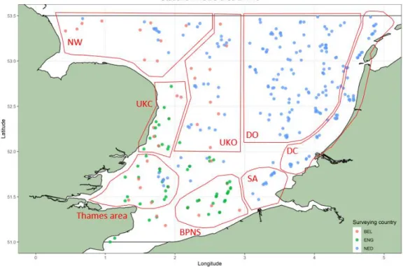
The analysis focused on the southern North Sea, which corresponds to ICES area 27.4.c (defined as the part of the North Sea between 51°N and 53.5°N, see Figure 1) and in the period 2006 – 2018. The selected dataset contains information from 3 research vessels. More details on the sampling gear, period and conditions are listed in Table 1 and can be found in ICES. 2018.
To make the description of spatial patterns easier and more concise, the map of ICES area 27.4.c was divided into multiple regions (Figure 1). The regions northwest of The Wash, the Inner Silver Pit and the Norfolk banks are described as ‘NW’. The coast of the United Kingdom is termed ‘UKC’, while the UK offshore area is named ‘UKO’. The ‘Thames area’
describes the mouth of the Thames. ‘BPNS’ stands for the Belgian Part of the North Sea, while ‘SA’ stands for the Scheldt area. The Dutch coast is labeled as ‘DC’, while the Dutch offshore area is termed ‘DO’. Sampling stations are sampled by different countries: stations indicated in red are sampled by the Belgian survey (BEL), stations in green are sampled by the English survey (ENG) and stations in blue are sampled by the Dutch survey (NED).
The dataset was quality checked by removing invalid hauls, by making the length classes uniform (different countries measure the length of a fish differently), by adding a column with the width of the beam trawl and by manually setting the groundspeed while fishing to 4 knots if it wasn’t recorded (groundspeed is used for calculating CPUE values). Using the World Register of Marine Species (WoRMS) (http://www.marinespecies.org; library
Figure 1: ICES area 27.4.c between 51°N and 53.5°N and the different sampling stations. Colours indicate which countries sample the station.
Country Research Vessel Sampling gear Gear position Sampling period
Belgium RV Belgica 4 m beam trawl Aft August – early September
United Kingdom RV Endeavour 4 m beam trawl Aft Late July
The Netherlands RV Tridens 8 m beam trawl Portside or starboard August – early September
Trawl duration Tow speed Cod-end stretched mesh N° of stations
Belgium 30 minutes 4 knots 40 mm 62
United Kingdom 30 minutes 4 knots 75 mm 100
The Netherlands 30 minutes 4 knots 40 mm 88
Material and methods Manu Claessens 7
(‘worms’) in R (Holstein 2018)), species codes were converted to scientific names. Non-fish species were removed from the dataset.
The dataset was divided into a numerical and a gravimetric dataset. When the length of a fish is known, the biomass can be calculated using the formula
𝑊𝑒𝑖𝑔ℎ𝑡 = 𝑎 ∗ 𝐿𝑒𝑛𝑔𝑡ℎ𝑏.
So-called ‘length-weight keys’, which provide the species-specific values for the parameters ‘a’ and ‘b’, allow to calculate the weight of individual fish based on their length. The ‘a’ and ‘b’ parameters were derived from Silva et al. 2013, which contains an extensive library of the length-weight relationships of marine fish collected around the British Isles. Subsequently, all fish species were classified as ‘commercial’ or ‘non-commercial’ using a rapport of landed species in 2018 (Velghe and Scherrens 2018). The non-commercial fish species were defined as species that were not landed in the fish auction. The commercial fish species were further divided into two subsets: ‘marketable’ and ‘undersized’ individuals. Marketable specimens have a size equal to or larger than the ‘minimum conservation reference size’ or ‘MCRS’ as obtained from the Council Regulation (EC) No 2015/812 (Salomon et al. 2014). The MCRS is a species-specific minimum length at which fish species are permitted to be landed in absence of the European landing obligation. The MCRS for plaice for example is 27 cm. Undersized individuals have a length smaller than the MCRS.
The environmental dataset was derived from the ICES DATRAS platform and from the Copernicus
Marine Service platform
(https://marine.copernicus.eu). Data analysis
For the analysis of this master’s dissertation, R version 3.6.1 was used (R Core Team 2019), accompanied by several packages (see Appendix). The most frequently used packages were part of the ‘tidyverse’ collection (Wickham et al. 2019), which was applied for data exploration, transformation, manipulation and plotting. A summary of the used code can also be found in Appendix.
The swept area per haul was calculated using the ground speed of the ship while towing (in knots or nautical miles per hour), the haul duration (in minutes) and the width of the beam (in meters) and converted to km2. The ‘Catch Per Unit Effort’
(‘CPUE’), which was used for comparisons between hauls, was calculated per species as the total weight of that species in a haul divided by the swept area in that same haul. The unit for CPUE is kg/km2.
Analysis of the spatiotemporal patterns of fish
communities in the North Sea was done by 1) performing a PCA and subsequent cluster analysis,
2) calculating diversity and evenness indices and 3) analysing which environmental variables are
explanatory for any observed spatiotemporal patterns.
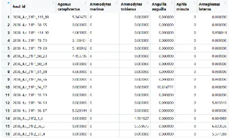
The rows of the dataset, which represent an individual caught during the beam trawl surveys, were grouped by year, sampling station, unique haul and species. If applicable, a distinction between marketable and undersized individuals was made. Next, the CPUE for this grouping was calculated and saved per species and per unique haul. The dataset was transposed and transformed (Figure 2): the unique hauls form the rows in this dataset, while the individual fish species make up the columns, with the CPUE for the aforementioned grouping in the cells. The ‘haul_id’, a string variable which contains the year (example for the first row: 2006), the ICES area (4.c), the ICES statistical rectangle (31F1), the sampling station (119) and the haul number (89), was made to be able to distinguish between the different hauls.
II.1) Analysis of fish communities
A PCA or ‘principal components analysis’ was used to reduce the multidimensionality of the transformed dataset. A PCA is a multivariate method of analysis that describes a large amount of data using a smaller number of variables, the so-called ‘principal components’ or ‘PCs’. The ‘PCA’ function in R belongs to the ‘FactoMineR’ package (Le et al. 2008) and was used to run a PCA on the transformed dataset. Before running the PCA, the CPUE values were 4th
root transformed to remove skew in the dataset caused by hauls with a disproportionately high CPUE. Subsequently, the ‘Hierarchical Clustering on Principal Components’ or ‘HCPC’ function in R, which also belongs to the ‘FactoMineR’ package, was used
8 Manu Claessens Material and methods
to perform a hierarchical clustering on the principal components obtained with the principal component analysis. The ‘HCPC’ function provides the user with useful graphs such as scree plots, dendrograms and PCA biplots. Clustering of the hauls was performed for each year (2006 – 2018). The choice of the number of clusters was arbitrarily set to 10.
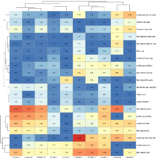
The 20 species shown in the heatmap (Figure 3) were chosen as follows. For each species in the dataset, the average CPUE per cluster was calculated in the clustering protocol. Next, these averages were summed over the clusters to get an indication which species contribute the most to defining the spatial pattern. The 20 species that had the highest summed value were chosen; marketable and undersized individuals of the same species were treated as two different species.
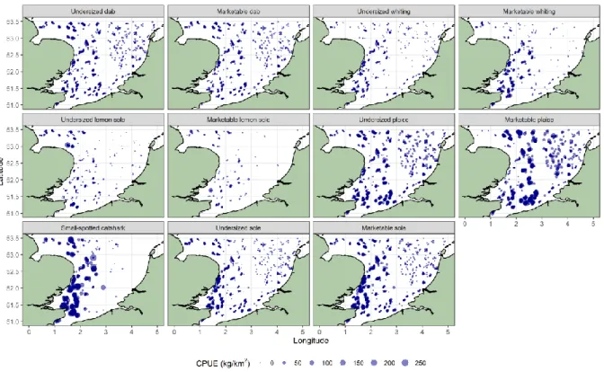
The spatial pattern of the multivariate cluster analysis was plotted by aggregating the sampling stations and clusters to which they were assigned to over the entire time series (2006 – 2018) (Figure 4). The spatial distribution of six fish species was analysed in-depth (Figure 5). First, species with an average CPUE in any cluster above 10 kg/km2 were
picked. Next, of the commercial species, both the marketable and the undersized individuals were chosen. For all analyses focused on these six species, a distinction between marketable and undersized individuals was made, if applicable.
The annual variation of fish communities was analysed by focusing on the same six fish species (Figure 6). The data was grouped by year, species and cluster. Calculations for all other species were grouped under ‘Other’.
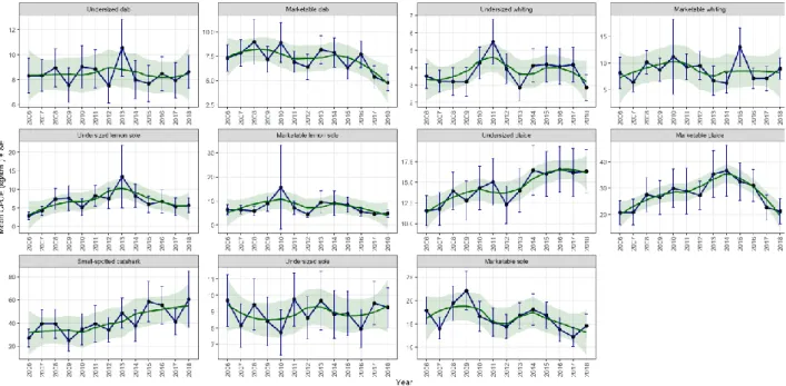
Temporal trends of the CPUE of six fish species were analysed in-depth as well (Figure 7). The data was grouped by year and species. Error bars of 95% confidence interval were added, as well as a loess smoother with SE values.
II.2) Analysis of diversity and evenness
The diversity at each sampling station was calculated using Hill’s diversity indices (Hill 1973) and an evenness index for each sampling station (protocol from
https://www.flutterbys.com.au/stats/tut/tut13.2.ht ml):
- N0: the species richness indicates the
number of unique species in a sample. It is calculated as the sum of all unique species; - N1: the exponent of the Shannon-Wiener
diversity index H’ (ln based) takes both the number of species and the relative abundances of those species into account:
𝐻′ = − ∑ (𝑛𝑖
𝑁× 𝑙𝑛 𝑛𝑖
𝑁) ; 𝑁1 = 𝑒
𝐻′;
- N2: the inverse of the Simpson diversity
index λ is a measure of the dominance of species. Higher values of N2 indicate a
community with a higher diversity:
𝜆 = ∑𝑛𝑖(𝑛𝑖− 1) 𝑁(𝑁 − 1) ; 𝑁2=
1 𝜆;
Results Manu Claessens 9
- J’: Pielou evenness of the Shannon-Wiener index H’ indicates how even the community is. The more variation in abundances between different taxa within the community, the lower the value of J will be:
𝐽′= 𝐻 ′ 𝑙𝑛(𝑆)= 𝐻′ 𝑙𝑛(𝑁0) .
Spatial patterns of the diversity indices and evenness index were visualized by considering the entire time series (2006 – 2018) (Figure 8).
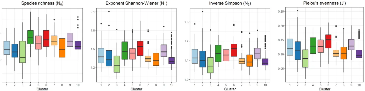
When summarizing spatial patterns of the diversity indices and evenness index, median values were used instead of mean values to avoid skewness in the data. Boxplots of diversity and evenness per cluster were made by grouping the stations that were assigned to each cluster and plotting Hill’s diversity indices and the evenness index calculated for those stations (Figure 9). The plot of the diversity and evenness per cluster over time was made similarly; the year was added as another grouping variable and the median value per cluster and per year was plotted (Figure 10).
II.3) Incorporating environmental variables
Spatial patterns of the environmental variables were visualized by pooling the entire time series (2006 – 2018) (Figure 11).
Boxplots of the different environmental variables per cluster were made by grouping the stations that were assigned to each cluster and plotting the environmental variables for those stations (Figure 12). Data was pooled over the period 2006 – 2018 to make up for the limited amount of observations per year in the environmental dataset.
Differences in the environmental variables between the different clusters were statistically tested for using an ANOVA (‘aov’ function belonging to the ‘car’ package (Fox and Weisberg 2019) in R). Homogeneity of variances was tested for using Levene's test (‘leveneTest’ function belonging to the ‘car’ package in R). The nonparametric Games-Howell post-hoc test (‘oneway’ function belonging to the ‘userfriendlyscience’ package (Peters 2018) in R) was used to compare combinations of clusters. P values were reported as following: ns (p > 0.05), * (p ≤ 0.05), ** (p ≤ 0.01) and *** (p ≤ 0.001).
To test what environmental variables were explaining the allocation of stations to a certain cluster, a multinomial logistic regression was applied. Protocol was largely followed from UCLA: Statistical Consulting Group. The clusters were used as the dependent variable, while the environmental variables were used as independent, predictor variables. Cluster one was chosen as the baseline outcome level (i.e. the cluster); all other clusters were therefore contrasted with cluster 1. Model selection was done using an automatic stepwise forward and backward selection procedure of the best fitting model by comparing ‘Akaike information criterion’ or ‘AIC’ values. Absence of collinearity between these three variables was tested for using a correlation test. P-values for the different regression coefficients were calculated with two-tailed z test using the coefficients and the standard errors extracted from the output of the multinomial logistic regression (Figure 13).
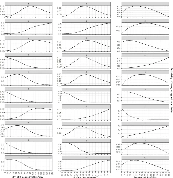
Probabilities of assigning a sampling station to a certain cluster based on the environmental variables were predicted (Figure 14) was done as follows. For each environmental variable, a probability plot was made. The mean of the other two variables was used to keep the other two variables constant. The ‘predict’ function in R was used to predict the probabilities based on the full model and the range of values the environmental variable under analysis can take. This way, only one environmental variable was taken into consideration at a time. The process was repeated for the other two environmental variables.
Results
Analysis of fish communities I.1) Identifying clusters
The cluster analysis shows that the 10 clusters can be grouped in 4 branches (Figure 3), where the clusters form the sub-branches. The first branch consists of clusters 8, 9 and 10, which are characterised by large catch rates of plaice and dab, both marketable and undersized. The second branch contains clusters 3 and 7, which have the lowest catch rates of these 20 most abundant species and show moderate CPUE values for both marketable and undersized sole. The third branch consists of clusters 1, 2 and 5,
10 Manu Claessens Results
Figure 3: Heatmap of the different clusters and the 20 species that contribute the most to defining the different clusters. Species are split between
marketable and undersized individuals if MCRS is defined. Values and their concurrent colours represent the mean CPUE (kg/km2) for each species in
each cluster. Selection of species: see Material and methods.
Figure 4: Spatial pattern of the multivariate cluster analysis (colours represent clusters as defined in the cluster analysis aggregated over the entire
Results Manu Claessens 11
Figure 5: CPUE (kg/km2) of dab, whiting, lemon sole, plaice, sole and catshark in the southern North Sea (2006 – 2018) with indication of
marketable and undersized fish, if applicable.
Figure 6: Relative CPUE contribution of dab, whiting, lemon sole, plaice, sole, catshark and all other species in the southern North Sea to each
12 Manu Claessens Results
characterised by the highest catch rates for sole (both marketable and undersized) and catshark. The fourth and last branch containing clusters 4 and 6 is characterised by high catch rates of catshark, but also dab (marketable and undersized), lemon sole (Microstomus kitt), armed bullhead (Agonus cataphractus), dragonet and whiting are caught a lot (mean per cluster > 5 kg/km2).
I.2) Spatial pattern of fish communities
The spatial distribution of fish communities based on the 10 clusters exhibits a clear east-west pattern (Figure 4). Clusters dominated by plaice and dab (specifically clusters 8 and 10) are generally found in the eastern parts of ICES area 27.4.c, while clusters that are dominated by sole and catshark (specifically cluster 1 and 2) are mainly found in the southwestern parts of that same area.
The offshore part of the eastern North Sea is dominated by plaice and dab (clusters 8 and 10 in the DO area and the BPNS), while European flounder (Platichthys flesus) has the highest catches in the coastal part of the eastern North Sea (cluster 7 in the DC and the SA). These patterns are contrasted by the southwestern North Sea, which is largely dominated by clusters with catshark and sole (clusters 1, 2 and 5 in the UKC area). Cluster 3, which shares the same sub-branch with cluster 7, is situated in the Thames area, the UKC area and the NW area and has intermediate catches of sole, plaice and dab. Cluster 9 in the NW area shows characteristics of both the western area (higher catches of marketable sole) and the eastern area (higher catches of dab and plaice) of the North Sea.
Clusters 4 and 6 cannot be associated with a specific geographical location and are more spread over the entire study area. Cluster 4 can be found in the BPNS, the NW area, the Thames area and the UKC area, while cluster 6 can be found in the NW area, but also in the Thames area and the DC area. Cluster 4 is characterised by marketable plaice, catshark, marketable whiting, marketable Atlantic cod and marketable lemon sole, in descending importance, while both marketable and undersized sole are completely absent from cluster 4.
The spatial distribution of six species was analysed in-depth: dab, whiting, lemon sole, plaice, sole and catshark (Figure 5). Generally, marketable individuals show higher abundances in offshore
areas and undersized individuals have higher abundances near the coasts. This is especially true for plaice and sole. Hauls of dab have a higher CPUE in the UKC, the UKO, the NW, the BPNS and the Thames area than in the DO or the DC areas. The same spatial patterns are found for whiting and lemon sole. Catshark has high abundances in the Thames area, the UKC area and to a lesser degree in the NW area, while catshark is absent in the eastern parts of ICES area 27.4.c.
The highest CPUE for marketable plaice is found in the BPNS (223.59 kg/km2), while the highest CPUE
for marketable sole is found in the Thames area (90.17 kg/km2). Undersized dab (8.44 ± 0.21 kg/km2)
has a higher CPUE than marketable dab (7.21 ± 0.20 kg/km2). For all other species under consideration,
the abundances of the marketable specimens are higher than the abundances of the undersized specimens.
I.3) Annual variation of fish communities
The pattern seen on Figure 4 is recognizable in the relative CPUE contributions of the different species to each cluster (Figure 6). Plaice and dab contribute a lot to clusters 8, 9 and 10, while sole and catshark contribute more to clusters 1 and 2.
Clusters 4 and 6, the two clusters with an inconsistent spatial distribution, are not dominated by a single species. Moreover, clusters 4 and 6 were not assigned in some of the analysed years. Cluster 4 is absent from Figure 6 in 2009 and 2016, while cluster 6 is absent in 2008, 2009 and 2015. Lemon sole stands out as a species that contributes a lot to clusters 4 and 6, but also as a species with a lot of interannual variation.
In general, the relative CPUE contribution of the different species to each cluster shows a lot of interannual variation.
Catshark has the highest mean CPUE of the selected species under study (60.56 ± 12.27 kg/km2 in 2018)
(Figure 7). The year significantly predicts the mean CPUE of catshark (t(11) = 3.699, p < 0.05). Of the commercial species, marketable plaice has the highest mean CPUE (36.63 ± 4.91 kg/km2 in 2014).
The year significantly predicts the mean CPUE of undersized plaice (t(11) = 5.467, p < 0.001), ranging from 11.56 ± 0.94 kg/km2 in 2006 to 16.58 ± 1.40
kg/km2 in 2016. The year also significantly predicts
Results Manu Claessens 13
p < 0.05), ranging from 8.99 ± 1.78 kg/km2 in 2008 to
4.80 ± 0.42 kg/km2. Other species do not show a
significant positive or negative trend between 2006 and 2018 (t(11) ranged from -1.942 to 0.867, p > 0.05).
Analysis of diversity and evenness
II.1) Spatial pattern of diversity and evenness Species richness (N0) is higher in coastal areas than
in offshore areas (Figure 8). The Thames area has a lower species richness (min-max: 3 to 23, median = 13) than the BPNS and the SA (min-max: 6 to 26, median = 16). The number of species in the NW area ranges from 6 to 27 with a median value of 16. The same pattern is reflected in the Hill’s index N1, which
is higher in the eastern part of the North Sea. N1 is
low in the DO area and the UKC area, similarly to the distribution pattern of N0. The inverse of the
Simpson index (N2) is the highest near the coasts,
especially south of the Thames area and off the BPNS. The distribution of J’, Pielou’s evenness, follows a similar pattern as N1.
Linking these diversity and evenness indices to the identified clusters showed high median values for N0,
N1, N2 and J’ in clusters 4 and 6, which are the two
clusters that lack a specific associated geographical location (Figure 9). Cluster 4 has the highest median
species richness N0 (min-max: 11 to 28,
median = 18.5), followed by cluster 6 (min-max: 11 to 27, median = 17.5). In comparison, cluster 1 (min-max: 8 to 22, median = 14), cluster 2 (min-(min-max: 6 to 22, median = 13) and cluster 3 (min-max: 3 to 24, median = 11) have a lower median species richness. Cluster 5 (min-max: 8 to 26, median = 16), cluster 6 max: 11 to 27, median = 17) and cluster 7 (min-max: 11 to 25, median = 17) have a higher median species richness.
Clusters 8 and 10 have intermediate median values for the species richness (14 and 15 respectively), while median values for N1 (1.31 and 1.30
respectively) and J’ (0.10 and 0.10) are low. Cluster 6 stands out with a high value for N1 (min-max: 1.20 to
1.96, median = 1.54), cluster 3 has the lowest values for N1 (min-max: 1.02 to 1.81, median = 1.23). The
pattern of J’, Pielou’s evenness index, follows that of
N1, with cluster 6 having the highest median J’ values
(min-max: 0.07 to 0.21, median = 0.15). Cluster 9 has median values for N0 (17), N1 (1.45) and N2 (1.13)
similar to those of cluster 5.
II.2) Temporal pattern of diversity and evenness No temporal pattern in the diversity and evenness between the different clusters can be distinguished (Figure 10). All four median index values are high for clusters 4 and 6, except for 2007 and 2015 and the years when these clusters were not assigned.
Incorporating environmental variables III.1) Spatial pattern of environmental variables NPP measurements are higher near the coasts (DC area, BPNS, Thames area) than in offshore areas (UKO area, NW area), with a maximum measured value of 236.33 mgC m−2 day−1 in the DC area (Figure
11). Surface temperatures are the highest in the eastern part of ICES area 27.4.c and the lowest in the NW area. Surface salinity on the other hand is the highest in offshore areas such as the UKO area and the NW area.
III.2) Linking clusters and environmental variables Cluster 7 stands out when looking at the differences of environmental variables between the different clusters (Figure 12). The median net primary production or NPP (min-max: 31.31 to 236.33 mgC m−2 day−1, median = 104.63 mgC m−2 day−1) and the
median surface temperature (min-max: 17.1 to 21.5 °C, median = 19.2 °C) in cluster 7 are higher than in other clusters, while the median surface salinity (min-max: 31.24 to 34.99 PSU, median = 33.64 PSU) is lower than that in the other clusters. Cluster 1 (min-max: 28.80 to 149.30 mgC m−2 day−1, median =
64.95 mgC m−2 day−1), cluster 2 (min-max: 24.47 to
169.60 mgC m−2 day−1, median = 82.48 mgC m−2
day−1) and cluster 3 (min-max: 11.59 to 155.25 mgC
m−2 day−1, median = 66.24 mgC m−2 day−1) also seem
to have a higher median value for NPP than the other clusters.
14 Manu Claessens Results
Figure 7: Mean CPUE of dab, whiting, lemon sole, plaice, sole and catshark per year with indication of marketable and undersized individuals if
applicable. Note the different scales on the y axes.
Figure 8: Spatial pattern of diversity and evenness per sampling station (2006 – 2018). Top left: species richness (N0);
Results Manu Claessens 15
Figure 9: Diversity and evenness per cluster (2006 – 2018). From left to right: species richness (N0); exponent Shannon-Wiener (N1);
inverse Simpson (N2); Pielou’s evenness (J’).
Figure 10: Median diversity and evenness per year for each cluster. Top left: species richness (N0); top right: exponent Shannon-Wiener (N1);
bottom left: inverse Simpson (N2); bottom right: Pielou’s evenness (J’).
Figure 11: Spatial pattern of environmental variables per sampling station (2006 – 2018). From left to right: net primary production at the
16 Manu Claessens Results
The NPP (ANOVA; F = 537.7, p < 0.001), the surface temperature (ANOVA; F = 401.7, p < 0.001) and the surface salinity (ANOVA; F = 65.12, p < 0.001) differ significantly between the different clusters.
Homogeneity of variances was rejected for the NPP ANOVA (F = 100.07, p < 0.001), for the surface temperature ANOVA (F = 37.28, p < 0.001) and for the surface salinity ANOVA (F = 18.82, p < 0.001). Games-Howell post-hoc tests were used to compare combinations of clusters; results are listed in Tables 2, 3 and 4.
A multinomial logistic regression model with all three environmental variables was chosen over a simpler model with only one or a combination of two out of three environmental variables, based on the AIC values. Correlations between the three different environmental variables under consideration are
weak: NPP~°t = 0.32, NPP~PSU = -0.15 and °t~PSU = -0.21.
The two-tailed z-tests of the different regression coefficients show that most regression coefficients
are significant, except for the surface temperature for clusters 4 (p > 0.05) and 5 (p > 0.05) (Figure 13). The probabilities of assigning a sampling station to a certain cluster based on the environmental variables are generally low (Figure 14). Low NPP values indicate a higher probability of assigning sampling stations to clusters 4, 5, 6, 8, 9 and 10; high NPP values indicate a higher probability of assigning sampling stations to clusters 2 (highest probability), 3 and 7. Low surface temperatures indicate a higher probability of assigning sampling stations to clusters 6 and 9; intermediate surface temperatures indicate a higher probability of assigning sampling stations to clusters 1, 3, 4, 5 and 8; high surface temperatures indicate a higher probability of assigning sampling stations to clusters 2, 7 and 10. Low surface salinities indicate a higher probability of assigning sampling stations to clusters 3, 6 and 7; intermediate surface salinities indicate a higher probability of assigning sampling stations to clusters 1, 2, 5, 9 and 10; high surface salinities indicate a higher probability of assigning sampling stations to clusters 4 and 8.
Results Manu Claessens 17
Figure 12: Environmental variables per cluster (2006 – 2018). From left to right: surface net primary production, surface temperature and surface
salinity. NPP 2 3 4 5 6 7 8 9 10 1 *** * *** *** *** *** *** *** *** 2 *** *** *** *** ns *** *** *** 3 *** *** *** *** *** *** *** 4 *** ns *** *** ** * 5 *** *** ns *** *** 6 *** *** ns *** 7 *** *** *** 8 *** ** 9 *** t° 2 3 4 5 6 7 8 9 10 1 *** * ns ns *** *** *** *** *** 2 *** *** *** *** *** *** *** *** 3 *** * *** *** *** *** ns 4 ** *** *** ns *** *** 5 *** *** *** *** *** 6 *** *** * *** 7 *** *** *** 8 *** *** 9 *** PSU 2 3 4 5 6 7 8 9 10 1 ns ns *** ns ns *** *** *** ns 2 ns *** *** ns *** *** *** ** 3 *** *** ns *** *** ** * 4 *** *** *** ns *** *** 5 ns *** *** ns ns 6 *** *** ** ns 7 *** *** *** 8 *** *** 9 ***
Tables 2, 3 and 4: Results of Games-Howell post-hoc tests of differences in surface net primary production (top), surface temperature (mid) and
18 Manu Claessens Results
(Intercept) SurTemp SurSal nppv_depth_0 2 0.000000e+00 0.0000000000 4.816671e-02 0.000000e+00 3 9.735324e-01 0.0024726034 2.737727e-02 2.345556e-05 4 2.984279e-13 0.7151683792 0.000000e+00 0.000000e+00 5 8.012982e-01 0.0640651941 1.601407e-01 0.000000e+00 6 0.000000e+00 0.0000000000 2.160955e-05 0.000000e+00 7 0.000000e+00 0.0000000000 0.000000e+00 7.184079e-05 8 2.012601e-06 0.0008166036 0.000000e+00 0.000000e+00 9 0.000000e+00 0.0000000000 3.816352e-01 0.000000e+00 10 1.856706e-06 0.0000000000 5.285587e-01 0.000000e+00
Figure 13: Two-tailed z tests of the output of the multinomial logistic regression. Comparisons with cluster 1 as baseline outcome level.
Figure 14: Probabilities for stations being assigned to a cluster based on environmental variables. From left to right: surface net primary
Discussion Manu Claessens 19
Discussion
Based on biomass measurements derived from scientific beam trawl surveys (ICES DATRAS database), several species assemblages were identified. Clusters dominated by plaice and dab were generally found in the eastern parts of the southern North Sea, while clusters characterised by sole and catshark were mostly found in the southwestern parts of the southern North Sea. The findings on the spatial distribution of plaice and sole in this thesis corroborate with Engelhard et al. 2011, who indicated that plaice and sole are characteristic species of the southern North Sea. Juvenile plaice uses coastal waters as nursery areas and moves offshore to deeper, cooler waters while maturing (Teal 2011). Plaice is a common species in the southern North Sea and in the German Bight (ICES. 2017 (Working Group on Assessment of Demersal Stocks in the North Sea and Skagerrak or WGNSSK)). In this master’s dissertation, undersized plaice was more abundant near the coasts, while marketable plaice had higher abundances in offshore areas. Despite these differences in spatial distribution, marketable and undersized plaice where usually assigned to the same cluster (e.g. clusters 5, 8, 9 and 10), with some exceptions (see further). Clusters dominated by plaice were found in the east of the study area, with the Dutch coast as an exception, where plaice’s importance was lower and marketable flounder played an important role. Like plaice, mature sole tends to inhabit deeper waters than the juveniles, although sole remains restricted to waters shallower than 50 meters, preferring sandy/muddy habitats across the North Sea (Teal 2011). Abundances of both marketable and undersized sole were higher in coastal clusters than in offshore clusters and generally higher in the west than in the east of the southern North Sea. Marketable and undersized sole were often assigned to the same cluster (e.g. clusters 1, 2 and 5).
Clusters dominated by plaice generally also had high contributions of sole, and vice versa. This reflects the large-scale distribution pattern of flatfish species in the North Sea, which have the highest abundances in the southern parts of the North Sea (Knijn et al. 1993, Callaway et al. 2002, Teal 2011). High numbers of juvenile specimens of flounder, sole, dab and plaice were reported in the Thames estuary (Power et al. 2000), indicating that flatfish species share the same
nursing and spawning grounds in the southern North Sea.
Apart from plaice and sole, four other species were identified as key contributors to the observed cluster pattern: dab, whiting, lemon sole and catshark. Dab showed an even distribution over the area under consideration. This matches with knowledge of dab as a generalist demersal fish species widely spread in the North Sea (ICES. 2017 (WGNSSK)), Sell and Kröncke 2013), with the highest abundances in the southeastern North Sea (ICES. 2017 (WGNSSK)). Whiting had higher abundances in the southwest of the southern North Sea. This is supported by ICES. 2017 (WGNSSK), where whiting showed the highest abundances in the southwestern North Sea. Whiting is known as a major fish predator in the North Sea ecosystem (Lauerburg et al. 2018) and is commonly found near the bottom in areas shallower than 200 meters (Teal 2011). Lemon sole had the lowest abundances of the six fish species under consideration. It was concentrated in the western parts of the study area and played an important role in characterizing clusters 4 and 6. Occurrences of lemon sole in the North Sea are most common at the Dogger Bank and at the Scottish coast (ICES. 2017 (WGNSSK)) and are positively correlated with depth in a study carried out on and near the Dogger Bank (Sell and Kröncke 2013). Catshark was the most abundant in the coastal, western parts of the studied region, which corresponds to findings that catfish is the most abundant on the continental shelves of the North Sea (ICES. 2017 (Working Group on Elasmobranchs or WGEF)).
Findings on the abundances of the six species analysed in this study does correspond to the latest report of the WGNSSK (ICES. 2017 (WGNSSK)) on the spatial distribution of those species. In many cases, there was also a match between the spatial distribution of individual species and the clusters they contributed most to. For example, the spatial distribution of sole and catshark abundances reflected the spatial pattern of the clusters they characterised. The match between the abundances of plaice and dab and the clusters they dominated was smaller.
Clusters 4 and 6 showed less consistent results. In some of the analysed years, these clusters were not assigned and the spatial distribution of clusters 4 and 6 was indistinct. A plausible explanation is that clusters were artificially divided due to the arbitrary
20 Manu Claessens Discussion
choice of working with 10 clusters. Yet, a rerun of the cluster analysis with 3, 7 or 12 clusters did not drastically change the observed patterns: a similar east-west pattern of different species assemblages was found, where plaice and dab dominated the eastern clusters and sole and catshark dominated the western clusters. This indicates the robustness of the clusters and confirms that the results derived from the multivariate analysis in this thesis are sturdy.
Mateo et al. 2017 set out to find spatially homogenous species assemblages in mixed demersal fisheries in the Celtic Sea and chose the most appropriate number of clusters for management purposes by applying the ‘elbow criterion’ (i.e. plotting the explained variation over the number of clusters and picking the elbow of the curve as the number of used clusters; adding another cluster beyond the ‘elbow’ does not explain the variance in the data better). Although this methodology is subjective and not always unambiguous (Ketchen and Shook 1996), it remains an easy to perform method to select the most adequate number of clusters. Mateo et al. 2017 worked with commercial haul data, but their methodology is also applicable to scientific survey data, such as the ICES DATRAS database which was used in this thesis. Therefore, future research on community patterns using a multivariate analysis should consider using the elbow criterion to choose the most fitting number of clusters. The choice of the number of clusters will also depend on the type of analysis: large-scale patterns can be identified using a limited number of clusters, while research on smaller-scale patterns will require a higher number of clusters.
Abundance trends over the years were significant for catshark (positive trend), undersized plaice (positive trend) and marketable dab (negative trend). The spawning stock biomass (the combined weight of all individuals in a stock that are capable of reproducing) of plaice in the North Sea and the Skagerrak has “markedly increased since 2008” (ICES. 2019). For this thesis, the temporal variations in biomass were of minor importance compared to the spatial patterns of biomass. The general cluster pattern remained relatively constant between 2006 and 2018, the span of the analysis. Whether the temporal variations in biomass formed an adequate
explanation for the inconsistencies of clusters 4 and 6 could not be concluded.
Samples near the coasts showed a high species richness, diversity and evenness, while offshore samples showed lower levels of species richness, diversity and evenness. The Thames area stood out as a region of samples with lower species richness than areas in the eastern parts of the southern North Sea, such as the BPNS and the SA. A higher diversity of fish species was reported for the shallower, southern parts of the North Sea compared to the deeper, northern parts of the North Sea (Callaway et al. 2002, Reiss et al. 2010, Frelat et al. 2017). Research of differences in species diversity specifically for the southern North Sea is not available: studies such as Reiss et al. 2010 focus on larger-scale patterns in the entire North Sea.
All environmental variables under consideration (surface net primary production, surface temperature and surface salinity) were measured in the 3rd quarter of the year. Each environmental
variable contributed significantly to explaining in which cluster each sampling station was categorized. Surface NPP was higher near the coasts than in offshores areas. Capuzzo et al. 2017 found high primary productivity in the southeastern parts of the North Sea (due to freshwater influence) and lower primary productivity in the southwest (permanently mixed waters), while van Denderen et al. 2014 reported higher yearly primary productivity near the DC area and the SA compared to offshore areas, which supports the findings of this thesis. Surface temperatures showed an increasing trend from the NW area to the BPNS, the SA and the DC area, while surface salinities were higher in offshore areas than near the coasts.
There was a match between the observed values of the environmental variables for each cluster and the predicted categorization based on those same environmental variables. Surface NPP for cluster 2 stood out: according to the probabilities derived from the multinomial logistic model, the probability of a sampling station being assigned to cluster 2 increased with increasing NPP to about 80%, while cluster 7 stood out from the preceding analysis as the cluster with the highest observed NPP. Probabilities were generally low, plausibly indicating that each environmental variable alone was not sufficient to accurately predict the assigned clusters.
Conclusions Manu Claessens 21
Demersal fish species exhibit differences in community composition between the northern and the southern regions of the North Sea: fish communities are separated by a boundary line between stratified northern and mixed southern water masses (Callaway et al. 2002, Fraser et al. 2008, Ehrich et al. 2009, Reiss et al. 2010, Teal 2011). There is strong support in favour of a link between hydrographical features (i.e. water masses, fronts, residual currents) and bottom fish assemblages (Ehrich et al. 2009). The relative influence of other environmental factors, such as depth, salinity, temperature and substrate, depends on the spatial scale and interactions between large- and local-scale processes (Menge and Olson 1990, Ehrich et al. 2009). Reiss et al. 2010 mark the importance of bottom water temperatures and thermal stratification of water columns in recognizing spatial patterns of infauna, epifauna and demersal fish communities. Sediment characteristics are less influential, and the impact of environmental variables is marked as scale-dependent, as indicated by earlier studies (Reiss et al. 2010). An older study highlights the role of fishing and its impact on the composition of fish communities (Roger et al. 1999). In this study, surface NPP, surface salinity and surface temperature all contributed significantly to defining the clusters. Adding more relevant environmental parameters such as hydrographical features, depth and substrate and sediment characteristics should improve predictions and might be an enticing option for future research.
The approach in this thesis made a distinction between non-commercial and commercial species and between marketable and undersized commercial species, which yielded interesting results. From a management perspective with the aim of reducing discards, some clusters stood out from the multivariate analysis. These clusters were typically characterised by marketable specimens, while undersized individuals of the same species were less important. Cluster 4 for example, found in the BPNS, the NW area, the Thames area and the UKC area, could be an interesting cluster for commercial fishery focused on plaice: it was characterised by marketable plaice, while undersized plaice was caught in lower abundances. Similarly, undersized sole had low abundances in clusters 6 and 9, making those clusters potentially attractive for commercial fishery targeted on sole.
Another interesting cluster in this study was cluster 7, which was typified by marketable and located in the DC area and the SA. This corresponds to findings from other studies: flounder is a typical species found in the coastal and estuarine areas of the North Sea (Knijn et al. 1993).
Conclusions
Recurrent fish species assemblages in the southern North Sea were identified using the ICES DATRAS database. Differentiating between marketable and undersized specimens of commercially sold species proved to be a possibility, which gives interesting prospects for future multivariate analyses. The spatiotemporal patterns of young individuals can be analysed separately from that of adult specimens, allowing for more detailed analyses of the distribution of commercially important fish species. Six species that played a key role in explaining the clusters were identified: dab, whiting, lemon sole, plaice, sole and catshark. A small selection of species seems sufficient to describe the spatiotemporal patterns of the communities they define. The analysis of species richness, diversity and evenness gave more insight into spatiotemporal patterns of fish species in the southern North Sea. Likewise, more knowledge on the role of environmental variables was gained by performing a multinomial logistic regression, revealing that surface net primary productivity, surface salinity and surface temperatures in the 3rd quarter significantly
contributed to explaining the assignment of sampling stations to the identified clusters. The implementation of more environmental variables such as depth, hydrological features and substrate characteristics to describe the spatiotemporal patterns of fish assemblages might improve predictions in future research.
Acknowledgements
As the author of this thesis, I would like to express my gratitude towards Marleen De Troch, Jochen Depestele and Lies Vansteenbrugge. This paper is the fruit of an intense cooperation with all three of my supervisors over an extended period of time. I would therefore like to thank them for keeping me motivated and on the lookout for possible improvements.
22 Manu Claessens References
References
North Sea cod recovery plan. (2001). Marine Pollution Bulletin, 42(3), 165-166.
Multinomial Logistic Regression. R Data Analysis Examples. UCLA: Statistical Consulting Group. from
https://stats.idre.ucla.edu/r/dae/multinomial-logistic-regression/.
Batsleer, J., Hamon, K. G., van Overzee, H. M. J., Rijnsdorp, A. D., & Poos, J. J. (2015). High-grading and over-quota discarding in mixed fisheries. Reviews in Fish Biology and Fisheries, 25(4), 715-736. doi:10.1007/s11160-015-9403-0
Beare, D., Rijnsdorp, A. D., Blaesberg, M., Damm, U., Egekvist, J., Fock, H., . . . Verweij, M. (2013). Evaluating the effect of fishery closures: Lessons learnt from the Plaice Box. Journal of Sea Research, 84, 49-60. doi:10.1016/j.seares.2013.04.002
Bellido, J. M., Santos, M. B., Pennino, M. G., Valeiras, X., & Pierce, G. J. (2011). Fishery discards and bycatch: solutions for an ecosystem approach to fisheries management? Hydrobiologia, 670(1), 317-333. doi:10.1007/s10750-011-0721-5
Bergman, M. J. N., & Lindeboom, H. J. (1999). Natural variability and the effects of fisheries in the North Sea: Towards an integrated fisheries and ecosystem management? Biogeochemical Cycling and Sediment Ecology, 59, 173-184.
Callaway, R., Alsvag, J., de Boois, I., Cotter, J., Ford, A., Hinz, H., . . . Ehrich, S. (2002). Diversity and community structure of epibenthic invertebrates and fish in the North Sea. Ices Journal of Marine
Science, 59(6), 1199-1214.
doi:10.1006/jmsc.2002.1288
Capuzzo, E., Lynam, C. P., Barry, J., Stephens, D., Forster, R. M., Greenwood, N., . . . Engelhard, G. H. (2018). A decline in primary production in the North Sea over 25 years, associated with reductions in zooplankton abundance and fish stock recruitment. Global Change Biology, 24(1), E352-E364. doi:10.1111/gcb.13916
Catchpole, T. L., Frid, C. L. J., & Gray, T. S. (2005). Discards in North Sea fisheries: causes, consequences and solutions. Marine Policy, 29(5), 421-430. doi:10.1016/j.marpol.2004.07.001
Catchpole, T. L., & Gray, T. S. (2010). Reducing discards of fish at sea: a review of European pilot projects. Journal of Environmental Management, 91(3), 717-723. doi:10.1016/j.jenvman.2009.09.035
Catchpole, T. L., Ribeiro-Santos, A., Mangi, S. C., Hedley, C., & Gray, T. S. (2017). The challenges of the landing obligation in EU fisheries. Marine Policy, 82, 76-86. doi:10.1016/j.marpol.2017.05.001
Cotter, A. J. R., Course, G., Buckland, S. T., & Garrod, C. (2002). A PPS sample survey of English fishing vessels to estimate discarding and retention of North Sea cod, haddock, and whiting. Fisheries Research, 55(1-3), 25-35. doi:Doi 10.1016/S0165-7836(01)00306-X
Davies, R. W. D., Cripps, S. J., Nickson, A., & Porter, G. (2009). Defining and estimating global marine fisheries bycatch. Marine Policy, 33(4), 661-672. doi:10.1016/j.marpol.2009.01.003
Daw, T., & Gray, T. (2005). Fisheries science and sustainability in international policy: a study of failure in the European Union's Common Fisheries Policy. Marine Policy, 29(3), 189-197. doi:10.1016/j.marpol.2004.03.003
de Vos, B. I., Doring, R., Aranda, M., Buisman, F. C., Frangoudes, K., Goti, L., . . . Vasilakopoulos, P. (2016). New modes of fisheries governance: Implementation of the landing obligation in four European countries. Marine Policy, 64, 1-8. doi:10.1016/j.marpol.2015.11.005
Depestele, J., Degrendele, K., Esmaeili, M., Ivanovic, A., Kroger, S., O'Neill, F. G., . . . Rijnsdorp, A. D. (2019). Comparison of mechanical disturbance in soft sediments due to tickler-chain SumWing trawl vs. electro-fitted PulseWing trawl. Ices Journal of Marine Science, 76(1), 312-329. doi:10.1093/icesjms/fsy124
Depestele, J., Desender, M., Benoit, H. P., Polet, H., & Vincx, M. (2014). Short-term survival of discarded target fish and non-target invertebrate species in the "eurocutter" beam trawl fishery of the southern North Sea. Fisheries Research, 154, 82-92. doi:10.1016/j.fishres.2014.01.018
EC. 2005. Council Regulation (EC) No 27/2005 of 22 December 2004 fixing for 2005 the fishing opportunities and associated conditions for certain fish stocks and groups of fish stocks, applicable in Community waters and, for Community vessels, in waters where catch limitations are required. Official Journal of the European Union, L 12/1–L 12/151.
Ehrich, S., Stelzenmuller, V., & Adlerstein, S. (2009). Linking spatial pattern of bottom fish assemblages with water masses in the North Sea. Fisheries Oceanography, 18(1), 36-50. doi:10.1111/j.1365-2419.2008.00495.x
References Manu Claessens 23
Engelhard, G. H., Lynam, C. P., Garcia-Carreras, B., Dolder, P. J., & Mackinson, S. (2015). Effort reduction and the large fish indicator: spatial trends reveal positive impacts of recent European fleet reduction schemes. Environmental Conservation, 42(3), 227-236. doi:10.1017/S0376892915000077
Evans, S. M., Hunter, J. E., Elizal, & Wahju, R. I. (1994). Composition and Fate of the Catch and Bycatch in the Farne-Deep (North-Sea) Nephrops Fishery. Ices Journal of Marine Science, 51(2), 155-168. doi:DOI 10.1006/jmsc.1994.1017
FAO. 2018. The State of World Fisheries and Aquaculture 2018 - Meeting the sustainable development goals. Rome. Licence: CC BY-NC-SA 3.0 IGO.
Fox, J., Weisberg, S. (2019). An {R} Companion to Applied Regression, Third Edition. Thousand Oaks
CA: Sage. URL:
https://socialsciences.mcmaster.ca/jfox/Books/Com panion/.
Fraser, H. M., Greenstreet, S. P. R., Fryer, R. J., & Piet, G. J. (2008). Mapping spatial variation in demersal fish species diversity and composition in the North Sea: accounting for species and size-related catchability in survey trawls. Ices Journal of Marine Science, 65(4), 531-538. doi:10.1093/icesjms/fsn036
Frelat, R., Lindegren, M., Denker, T. S., Floeter, J., Fock, H. O., Sguotti, C., . . . Mollmann, C. (2017). Community ecology in 3D: Tensor decomposition reveals spatio-temporal dynamics of large ecological communities. Plos One, 12(11). doi:ARTN e018820510.1371/journal.pone.0188205
Garthe, S., Camphuysen, C. J., & Furness, R. W. (1996). Amounts of discards by commercial fisheries and their significance as food for seabirds in the North Sea. Marine Ecology Progress Series, 136(1-3), 1-11. doi:DOI 10.3354/meps136001
Gray, T., Hatchard, J., Daw, T., & Stead, S. (2008). New cod war of words: 'Cod is God' versus 'sod the cod' - Two opposed discourses on the North Sea Cod Recovery Programme. Fisheries Research, 93(2), 1-7. doi:10.1016/j.fishres.2008.04.009
Guillen, J., Holmes, S. J., Carvalho, N., Casey, J., Dorner, H., Gibin, M., . . . Zanzi, A. (2018). A Review of the European Union Landing Obligation Focusing on Its Implications for Fisheries and the Environment. Sustainability, 10(4). doi:ARTN 900 10.3390/su10040900
Gullestad, P., Blom, G., Bakke, G., & Bogstad, B. (2015). The "Discard Ban Package": Experiences in efforts to improve the exploitation patterns in Norwegian fisheries. Marine Policy, 54, 1-9. doi:10.1016/j.marpol.2014.09.025
Hill, M. O. (1973). Diversity and Evenness: A Unifying Notation and Its Consequences. Ecology, 54(2), 427-432. doi:Doi 10.2307/1934352
Holstein, J. (2018). worms: Retriving Aphia Information from World Register of Marine Species. R package version 0.2.2. https://CRAN.R-project.org/package=worms.
Horwood, J., O'Brien, C., & Darby, C. (2006). North Sea cod recovery? Ices Journal of Marine Science, 63(6), 961-968. doi:10.1016/j.icesjms.2006.05.001
Horwood, J. W., Nichols, J. H., & Milligan, S. (1998). Evaluation of closed areas for fish stock conservation. Journal of Applied Ecology, 35(6), 893-903.
ICES. 2017. Report of the Working Group on Assessment of Demersal Stocks in the North Sea and Skagerrak (2017), 26 April–5 May 2017, ICES HQ. ICES CM 2017/ACOM:21. 1248 pp.
ICES. 2017. Report of the Working Group on Elasmobranchs (2017), 31 May-7 June 2017, Lisbon, Portugal. ICES CM 2017/ACOM:16. 1018 pp.
ICES. 2018. Report on the Working Group on Beam Trawl Surveys (WGBEAM). 10-13 April 2018. IJmuiden, Netherlands. ICES CM 2018/EOSG:05. 105 pp.
Kelleher, K. Discards in the world’s marine fisheries. An update. FAO Fisheries Technical Paper. No. 470. Rome, FAO. 2005. 131p.
Ketchen, D. J., & Shook, C. L. (1996). The application of cluster analysis in strategic management research: An analysis and critique. Strategic Management Journal, 17(6), 441-458.
doi:Doi
10.1002/(Sici)1097-0266(199606)17:6<441::Aid-Smj819>3.0.Co;2-G Larsen, R. B., Herrmann, B., Sistiaga, M., Grimaldo, E., Tatone, I., & Brinkhof, J. (2018). Size selection of cod (Gadus morhua) and haddock (Melanograrnrnus aeglefinus) in the Northeast Atlantic bottom trawl fishery with a newly developed double steel grid system. Fisheries Research, 201, 120-130. doi:10.1016/j.fishres.2018.01.021
Lauerburg, R. A. M., Temming, A., Pinnegar, J. K., Kotterba, P., Sell, A. F., Kempf, A., & Floeter, J. (2018). Forage fish control population dynamics of North Sea whiting Merlangius merlangus. Marine Ecology