Methods used to compensate for the effect of missing data in air quality measurements

(1)

(2)

(3)

Methods used to compensate

for the effect of missing data

in air quality measurements

RIVM Letter report 2014-0079 P.L. Nguyen│R. Hoogerbrugge

(4)

Colophon

Parts of this publication may be reproduced, provided acknowledgement is given to: National Institute for Public Health and the Environment, along with the title and year of publication.

P.L. Nguyen, RIVM

R. Hoogerbrugge (Project leader), RIVM

Contact: Lan Nguyen

Centre for Environmental Quality lan.nguyen@rivm.nl

This investigation has been performed by order and for the account of the Directorate-General Environmental protection, within the framework of the project 680704 Reporting Air Quality

This is a publication of:

National Institute for Public Health and the Environment

P.O. Box 1│3720 BA Bilthoven The Netherlands

(5)

Publiekssamenvatting

Methoden om het effect van ontbrekende data bij luchtkwaliteitsmetingen te ondervangen

Lidstaten van de Europese Unie zijn verplicht om de luchtkwaliteit te meten en te rapporteren. Belangrijk hierbij is de rapportage van de jaargemiddelde concentratie. Voor het berekenen van een geldig

jaargemiddelde geldt als criterium dat voor minimaal 90 % van de uren in een jaar een uur gemiddelde concentratie beschikbaar moet zijn. Als het aantal beschikbare uren niet aan het 90 % criterium voldoet mag een alternatieve methode gebruikt worden om het jaargemiddelde te berekenen. In dat verband heeft het RIVM voor stikstofdioxide en fijn stof een methode ontwikkeld. Op die manier kan, van een jaarreeks met een aanzienlijk aantal ontbrekende uurwaarden, toch een bruikbaar jaargemiddelde worden bepaald.

Het jaargemiddelde van gemeten concentraties stikstofdioxide en fijn stof is een belangrijke waarde en wordt voor twee doelen gebruikt: om trends te bepalen en om metingen te vergelijkingen met

modelberekeningen. Als uurwaarden ontbreken, heeft dit een effect op de nauwkeurigheid van het berekende jaargemiddelde. Uit RIVM-onderzoek blijkt dat dit effect sterk afhankelijk is van het ‘patroon’ van de ontbrekende meetgegevens en de methode waarmee de ontbrekende gegevens vervolgens worden behandeld. Als een aaneengeschakelde hoeveelheid meetgegevens ontbreekt, heeft dat een veel grotere invloed op de nauwkeurigheid dan eenzelfde hoeveelheid ontbrekende gegevens die verdeeld zijn over het jaar.

Voor de jaargemiddelde stikstofdioxide concentratie geldt, naast het criterium voor de databeschikbaarheid ook een onzekerheidscriterium van 15 %. Het jaargemiddelde van een dataset met een

aaneengeschakeld gat van 35 procent blijkt nog steeds aan de vereiste maximale onzekerheid van 15 procent te voldoen als de dataset wordt opgevuld volgens de methoden die het RIVM heeft ontwikkeld. Voor fijn stof (PM10) voldoet dan zelfs een dataset waarvan 75 procent van de data ontbreekt nog steeds aan de vereiste maximale onzekerheid van 25 procent.

(6)

(7)

Synopsis

Methods used to compensate for the effect of missing data in air quality measurements

Member States of the European Union are required to submit air-quality reports. Accordingly, the monitoring networks are required to store 90% of the requisite data. Member States are allowed to use supplementary methods for their air quality assessment. In this context, the Dutch National Institute for Public Health and the Environment (RIVM) has developed a method for nitrogen dioxide and particulate matter to compensate for the effect of missing data. With this method the

accuracy of the results are improved significantly and this method also makes it possible to calculate useful average annual concentrations. The annual averages of the measured concentrations of nitrogen dioxide and particulate matter are important values. They are used to identify trends and to compare the values obtained using models with actual measurements. If any hourly concentration measurements are missing, this will impact the accuracy of the calculated annual average

concentrations. An RIVM study has shown that the scale of this impact is highly dependent on the ‘pattern’ of missing measurement data and on the method used to compensate for such data. A consecutive series of missing data has a much greater impact on accuracy than the same quantity of missing data distributed throughout the year.

Even in the case of a nitrogen dioxide dataset with a 35% ‘block gap’, when the methods developed by RIVM were used to compensate for the missing data, the dataset’s annual average was shown to comply with the requisite maximum uncertainty of 15%. In the case of particulate matter (PM10), even datasets from which 75% of the data is missing can still comply with the required maximum uncertainty of 25%. Keywords: nitrogen dioxide, particulate matter, gap-filling

(8)

(9)

1 Introduction

In accordance with EU legislation, the air quality in the Netherlands is monitored by the Dutch national Air Quality Monitoring Network (LML). In addition to the national Air Quality Monitoring Network, the Municipal Health Service Amsterdam (GGD Amsterdam) and the Environmental Protection Agency Rijnmond (DCMR) have their own monitoring networks to monitor the air quality in these densely populated areas. Data of these networks are also used in reporting of air quality. For all pollutants the EU Directive 2008/50/EC prescribes for fixed

measurements a minimum data capture of 90%. However data sets with more than 10 % of missing data can be very useful. In the Netherlands a method to handle larger amounts of missing data is used in the assessment and reporting of Average Exposure Indicator (AEI) and the National Exposure Reduction Target (NERT) of PM2.5. Particularly in

calculating the AEI for the reference year (2010), in which annual concentrations in 2008, 2009 and 2010 are needed, difficulties were encountered because it was not possible to attain 90% data capture for all sites as part of the sampling points were not yet fully operational in 2008. In addition, in the National Air Quality Network measurements of PM2.5 are performed with the reference method (filter sampling and

weighing).This method has lower uncertainty compared to automatic measurements. However, as the filter collection is performed every 2 weeks, in case of failure of measurements, up to 2 weeks of data may be lost. Therefore, the National Institute for Public Health and the Environment (RIVM) has developed a gap-filling method for PM2.5

concentrations. This method is based on the strong correlation between PM2.5 over the Netherlands and is used in the calculation of the official

Dutch AEI (Mooibroek et al.,2013).

For reporting of other components a data capture of at least 90% is maintained although measurements with lower data capture might still be representative for the air quality at that location. Consequently, useful (expensive) data might be left out. In addition, sometimes, mobile equipment is used for monitoring of air quality at typical

locations. Mostly these measurements are not performed continuously because the equipment is only available for a short period or because it has to be used at another location. For such experiments it is relevant to plan measurements as such that representative air quality can be

obtained.

(12)

(13)

2 Set-up of this study

Hourly NO2 measurements and daily PM10 measurements in 2012 in the

LML, GGD monitoring network and the monitoring network of DCMR were used in this study. All measurements at rural sites, urban background sites and traffic related sites were used. Because

measurements at sites with data are used to gap-fill missing data at other sites, it is necessary to know which sites can be included in the model. For PM2.5 it was found that there is a strong correlation between

measurements over the Netherlands. Consequently, measurements of all sites can be used to fill missing data. However, as NO2 concentration

is influenced by local activities (traffic, urban activities) the use of measurements at comparable sites might have benefit. This aspect needs to be studied. The set-up of this study is therefore as follows:

- Gap-filling was performed with data set consisting of all sites as well as with data sets of each typical type (regional, urban background, traffic related).

- The data set was divided into 2 equal parts: half of the data set was kept as such1_{; in the other half of the data set, fictive}

missing data were created by deleting a part of measured data. This procedure is chosen to have sufficient data in the new data set. Both parts contain data of sites which are distributed over the whole Netherlands.

- The gap-filling was tested with 2 patterns of missing data. In one test missing data were distributed randomly over the whole year (random gaps); in another test one large block of data was removed (block gap), with a random start of the block at each site.

- Depending on the percentage of missing data (which ranged in this study from 20 to 75%) and the type of missing data (random versus block gap), several data sets were made. Table 1 shows the data sets used in this study.

(14)

Table 1: Data sets used in this study

Type sites Type gap % fictive missing data

All sites random 20-75

block 20-75

Rural random 20-75

block 20-75 Urban background random 20-75

block 20-75 Traffic related random 20-75

block 20-75

- All data sets were gap-filled by the “consistency method” This method is currently in use in The Netherlands in the in gap-filling of PM2.5 measuring data. . A brief description of this method is

given in the next chapter.

- In order to examine if better results can be obtained with a more complex method, data sets with 75% missing data were also filled by the Multiple Imputation method, using a tool which was also developed by the RIVM (Hoogerbrugge et al.,2000). In this report this method will be called “Mimp tool”. A brief description of this method is given in the next chapter.

- Annual concentrations were calculated and compared with original data.

- To evaluate the performance of the various methods the following indicators were calculated:

=

∑ , ,

₍₁₎

=

∑ , ,

₍₂₎

, , , ,

(3)

, , , ,

(4)

(15)

=

∑ ,

(5)

=

∑ ,

(6)

n: number of sites being gap-filled

C

meas,i: original annual concentration at site i

C

gap,i: annual concentration at site i after missing data were

created

C

filled,,i: annual concentration at site i after gap-filling of missing

data

Each gap-filling by the consistency method was performed ten times and the standard deviation of these runs was also determined.

(16)

(17)

3 Description of used gap-filling methods

3.1 Consistency method

The consistency method (Mooibroek et al.,RIVM report

680704022/2013) is based on the assumption that the concentration on day j for site i is proportional to the average of all measured

concentrations on that particular day. Since the measured

concentrations, xij may be different from the average of all sites ̅ the

contribution will be scaled by this proportion. Mathematically the

extension (expectation value) can be calculated using the expression (for daily concentration)2_:

= ̅ *

̅ ̿ where

̅ =

∑

̅ =

∑

̿ =

∑ ∑_∗

In these equations k is the number of sites and n = 366 the number of days in 2012. In the calculation of the averages the expectation values are used to substitute the missing values. In order to solve the above equation, a problem exists in that the averages used to calculate the expectation values are dependent on the expectation values themselves. Such a recursive relation can be solved by an initial calculation with some realistic starting values. The calculation is stopped after 100 iterations or when the difference between two iterations is less than 0.001.

For NO2 the same scheme is used however for hourly measurement values instead of daily values. Then n=366*24= 8784.

3.2 Multiple imputation method

In the multiple imputation algorithm (Geman and Geman, 1984) any missing value in principle is replaced by a model value. However, instead of the

model value itself a random value from a normal distribution around the model value is drawn. The standard deviation of this distribution is equal to the residual standard deviation between the model and the measured values.

2_{For NO}

(18)

This algorithm was implemented at RIVM both for handling missing data and for the handling of results below the detection limit. The approach was validated in the comparison with several other strategies on a nearly complete, but artificially censored data set of dioxins in cow’s milk (Hoogerbrugge and Liem, 2000). In that study the multiple

imputation algorithm appeared to have the smallest error of prediction and an adequate estimate for the uncertainty.

In the resulting iteration process the levels of the first location of all the samples of the dataset in which the data point is missing is modelled using the

concentrations of the other locations. The ‘old’ starting values on the positions of the missing data are replaced by new imputations. Then the concentrations of the second location are modelled and imputed and so on. After imputation of the last location the iteration is continued with re-imputating the first location etc. until the set number of iterations have been performed.

In the implementation of the multiple imputation as applied in this study the following choices were made:

the model for each location is generated using a regression model of the first

5 principal components (Principal Component Regression, PCR), (Massart, 1997). For the calculation of the principal components all other locations are used. Principal components are used to reduce the number of independent variables with a minimum loss of information. To avoid an underestimation of the uncertainty rather extreme starting values were chosen:

1) Normal distributed random data with mean and standard deviation of the detected values;

2) Equal to the largest concentration in the data set (max); 3) Equal to 0.01*max

4) Equal to 0.1*max.

The data are logtransformed3_{, which is in line with the assumption that}

the measurement uncertainty is proportional with the measured concentration.

The iterations are sufficient to obtain convergence between the four starting conditions.

3.3 No gap-filling

If missing data are not gap-filled, the yearly average is calculated based on the remaining data, i.e. for NO2 (where yearly average is calculated

from hourly data):

C gap,i=

̅ =

∑

Where

n: number of hours with data

Note that the result is equal to a data set where each missing value is assumed equal to the average of the measured data.

3_{If the minimum concentration at a site is negative, all data at that site are raised with 2 times of absolute}

(19)

4 Uncertainty of gap-filled data

For NO2 the Directive 2008/50/EC prescribes a maximum uncertainty of

15% (expressed at a confidence level of 95%). When data are gap-filled an additional uncertainty is introduced to the uncertainty of

measurements. The acceptable additional uncertainty need to be estimated.

At location i and time j the concentration is µij (for example µij is

average concentration of a large set of reference measurements) and the measurement is xij.

xij = µij - εij

For a yearly average the uncertainty umeas of measurements is: =∑ ̅

̅ , ̅ : measured yearly concentration and yearly concentration at location i in year j, respectively

k: number of locations

For NO2 umeas must be lower than 15%/2=7.5% and for PM10 umeas must

be lower than 25%/2=12.5%.

When missing data are gap-filled by estimated values mij the yearly

average of gap-filled data is 4_: ∑

366 for available measurement data for missing measurement data

The total uncertainty of a gap-filled dataset is:

=∑

with k: number of locations

=∑ ̅ ̅

=∑ ̅ _∑ _̅

2

∑ ̅ ̅

= + 2* corr* umeas* ufilled (7)

ufilled is additional uncertainty due to the gap-filling.

corr is the correlation coefficient between uncertainty of measurements and uncertainty due to gap-filling.

4_{For PM}

(20)

Simple situations: corr=0 : =

corr=1:

corr=-1:

Data of parallel measurements of RIVM and GGD (stations 14 and 543 in Amsterdam) and RIVM and DCMR (stations 448 and 493 in Rotterdam) were used for estimating of this correlation coefficient.

- The concentration at these locations is assumed to be equal to average of these parallel measurements and u meas was calculated

- In the dataset a block gap of 50% data were created and ufilled

and utot were calculated

- corr was calculated by equation (7)

Depending on the used dataset corr values ranging from -0.5 to 0.1 were found. Negative corr means that the yearly average of the gap-filled dataset is closer to the average of parallel measurements than individual measurement itself.

In the analysis in this report the uncertainties are estimated over a large part of the data set and assumed representative for each station. In areas with a large density of stations, the estimate may be more accurate than in areas with few stations. To study this effect a special calculation was made to gap-fill the data in Amsterdam by using only stations from other part of the country, i.e. Breda (station 241) and Groningen (station 938). Actually this was the only set with a positive but very small correlation (0.1) For more details see annex 1.

Based on these results, corr=0 seems to be a realistic assumption (even slightly conservative). The total uncertainty of a gap-filled data set becomes:

=

For NO2 the uncertainty of measured yearly concentration is estimated

at 11.2%(AQUILA,N256). For PM10 the uncertainty of measured yearly

concentration of automatic measurements is not known but the

uncertainty of measured daily concentration is estimated at 18% (at 50 µg/m3_{). For reference measurement (filter weighing) it is found that the}

uncertainty of yearly concentration (at 40 µg/m3_{) is lower than the}

uncertainty of daily concentration (at 50 µg/m3_{). For a conservative}

approach we assume that the uncertainty of yearly concentration of automatic measurement is equal to the uncertainty of daily

concentration, i.e. umeas of PM10 is estimated at 18% (at 40 µg/m3).

4.1 NO2

As the maximum total uncertainty is 15%, the acceptable uncertainty introduced by the gap-filling can be estimated as:

, (0.15)2-(0.112)2

i.e. ufilled,max=10%=40*0.1=4 µg/m3 (expressed at a confidence level of

95%) and the acceptable RMSE for EU reporting due to gap-filling is: 4.0/2=2µg/m3_{, at the limit value of 40 µg/m}3

(21)

In order to estimate an acceptable additional uncertainty which can be applied at each concentration level, RSD instead of RMSE should be used.

At limit value, the acceptable additional uncertainty is: ufilled,max=10%

(expressed at a confidence level of 95%),i.e. RSDfilled,max=5%

Relative standard deviation is often higher at lower concentration. Consequently if acceptable standard deviation is set at 5% at all

concentration levels, the results will be conservative, i.e. when the gap-filled data satisfy this requirement, there is no doubt that these data are representative. In the following chapters, the results of both indicators are shown. Since one indicator is in absolute units and the other relative both the high and the low end of the concentration range is covered. The critical values are small compared the measurement uncertainty and on average can be added to the measurement uncertainty without exceeding the EU maximum allowed uncertainty.

4.2 PM10

As the maximum total uncertainty is 25%, the acceptable uncertainty introduced by the gap-filling can be estimated as:

, (0.25)2-(0.18)2

i.e. ufilled,max=17%=40*0.17=6.8 µg/m3 (expressed at a confidence level

of 95%)

and the acceptable RMSE for EU reporting due to gap-filling is: 6.8/2=3.4µg/m3_{, at the limit value of 40 µg/m}3

In order to estimate an acceptable additional uncertainty which can be applied at each concentration level, RSD instead of RMSE should be used.

At limit value, the acceptable additional uncertainty is: ufilled,max=17%

(expressed at a confidence level of 95%),i.e. RSDfilled,max=8.5%

Relative standard deviation is often higher at lower concentration. Consequently if acceptable standard deviation is set at 8.5% at all concentration levels, the results will be conservative, i.e. when the gap-filled data satisfy this requirement, there is no doubt that these data are representative. In the following chapters, the results of both approaches are shown.

(22)

(23)

5 Results

5.1 All measurements sites in one data set

5.1.1 NO2data set

This data set consists of 63 sites. Data of 32 sites were kept as such. At 31 sites fictive missing data were created. In annex 2 the complete list of all the sites are given. The gap-filling with consistency method were performed ten times and all reported results are average of these 10 runs. In table 2 and 3 the results of gap-filling by consistency method was shown for various percentages of missing data. The Mimp tool was only applied in the most difficult test case (a block of 75% missing data) and was performed only once. As described in chapter 3, the Mimptool gives four solutions, depending on the start values. The results reported here are average of these four solutions.

Table 2: RMSE (in µg/m3_{) of annual average concentrations at various}

percentages of (fictive)missing data: without gap-filling, gap-filled by

consistency method and gap-filled by Mimp tool. The green cells show conditions

with RMSE <2 µg/m3

Random gaps Block gaps % fictive

missing data

RMSEgap RMSEfilled

(consistency method)

RMSEgap RMSEfilled

(consistency method) RMSEfilled (Mimp tool) 20 _0.09 _0.15 _1.26 _0.61 35 _0.14 _0.16 _2.20 _0.93 50 _0.20 _0.18 _3.27 _1.39 62.5 0.24 0.19 4.40 1.99 75 _0.32 _0.24 _4.97 _2.49 _1.45

Table 3: RSD of annual average concentrations at various percentages of (fictive) missing data: without gap-filling, gap-filled by consistency method and gap-filled by Mimp tool. The green cells show conditions with RSD <0.05

Random gaps Block gaps % fictive missing data RSDgap RSDfilled (consistency method) RSDgap RSDfilled (consistency method) RSDfilled (Mimp tool) 20 _0.003 _0.005 _0.053 _0.023 35 _0.005 _0.006 _0.090 _0.035 50 _0.007 _0.006 _0.139 _0.052 62.5 0.009 0.007 0.196 0.076 75 _0.011 _0.008 _0.225 _0.094 _0.049

Results in tables 2and 3 show:

- If missing data are distributed randomly, up to 75% missing data still don’t have significant effect on annual concentration, even

(24)

when missing data are unfilled. The RMSE is 0.32 µg/m3_{, which}

means that an additional uncertainty of 0.32*2/40=2% is introduced. The total uncertainty becomes:

sqrt(0.112*0.112+0.02*0.02)=11.4%. In this case the benefit of gap-filling is neglibible. However in real situations missing data are mostly not totally random. Small blocks of missing data which are randomly distributed are more realistic. A test on the evenly distribution of missing data can be done by comparison the actual distribution of missing data over hours, days, weeks, months with the expected distribution (see de Leeuw,2012 for more details).

- When a large block of data is missing, uncertainty becomes much larger. Gap-filling by consistency method reduces the uncertainty by a factor 2. If the data are not gap-filled, the constraint

RMSE<2 µg/m3 _{can be satisfied up to 20% missing data.}

However, as discussed above, the stricter requirement RSD<0.05 should be satisfied and gap-filling of data is necessary. Table 3 shows that with nearly 50% missing data this requirement is satisfied by the consistency method. When variations between runs are taken into account (shown by error bars in Figures 1A and 1B), the maximum acceptable percentage of missing data is some more than 35%.

- Compared to consistency method the Mimp tool seems to reduce the uncertainty by a factor 2 (however this is only determined at one point)

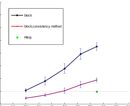
Figure 1A: RMSE as a function of percentage of missing data in data sets with block gaps. The error bar shows 2*standard deviations determined by 10 runs.

The line with RMSE=2 µg/m3_{is also shown.}

0 10 20 30 40 50 60 70 80 90 100 0 1 2 3 4 5 6 7 RM S E % missing data

NO₂ data, all sites

block

block,consistency method

(25)

Figure 1B: RSD as a function of percentage of missing data in data sets with block gaps. The error bar shows 2*standard deviations determined by 10 runs. The line with RSD=0.05 is also shown.

Figure 2 shows yearly concentrations of four individual solutions of the Mimptool as a function of original data. The figure shows a random distribution around the diagonal. With a small difference (mostly less than 1µg/m3_{) between four outputs of the Mimptool. This difference is}

significantly smaller than the difference between the average of the solutions and the original data set indicating that the uncertainty of the Mimp solution is underestimated.

Figure 2: yearly concentrations calculated by four individual solutions of the Mimptool

As an example figure 3 shows the hourly concentration of NO2 at station 448 (Bentinckplein) in Rotterdam. The gap-filling was performed by a

0 10 20 30 40 50 60 70 80 90 100 0 0.05 0.1 0.15 0.2 0.25 0.3 0.35 0.4 RS D % missing data NO

2 data, all sites

block block,consistency method Mimp 15 20 25 30 35 40 45 50 15 20 25 30 35 40 45 50 ga p-fi lled y ea rl y c on c en tr at io n

original yearly concentration NO₂ data, all sites

(26)

data set with block gaps of 35%. At this percentage the total uncertainty of gap-filled data sets is below the requirement of 15%. The figure shows that gap-filled data follows measured data quite well.

Figure 3: Gap-filled and measured hourly concentration at Bentinckplein (station 448, a traffic related location).The measured data block of the plot was (of course) not included in the data set used to calculate the gap filled data. 5.1.2 PM10 data set

This data set are daily concentrations of 79 sites. Because the effect of measurements type sites on PM10 concentration is much less

pronouncing, all monitoring sites were included in this set, i.e. including some industrial sites in the IJmond. In annex 1 the complete list of all sites are given. Data of 40 sites were kept as such. At 39 sites fictive missing data were created. The gap-filling with consistency method were performed ten times and all reported results are average of these 10 runs. In table 4 and 5 the results of gap-filling by consistency method was shown for various percentages of missing data. The Mimp tool was only applied in the most difficult test case (a block of 75% missing data) and was performed only once. As described in chapter 3, the Mimptool gives four solutions, depending on the start values. The results reported here are average of these four solutions.

(27)

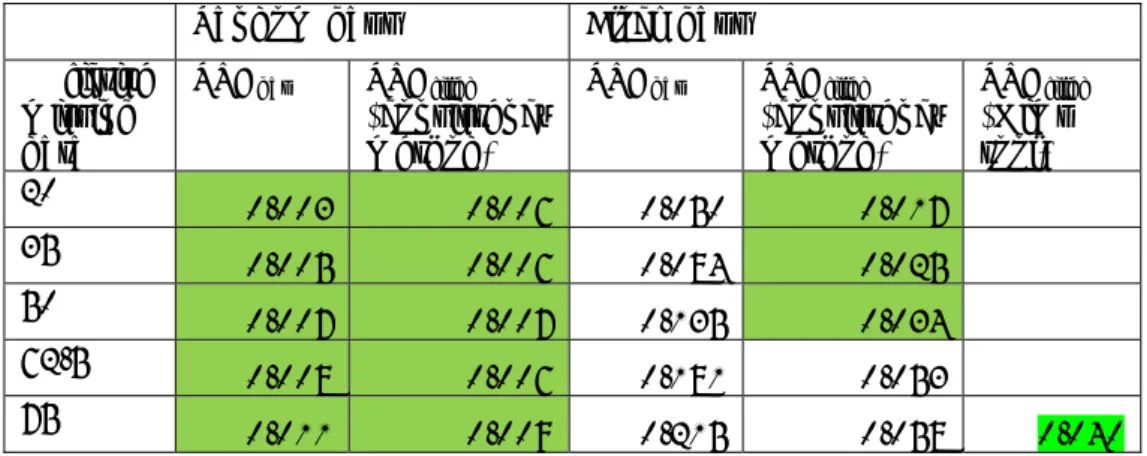
Table 4: RMSE (in µg/m3_{) of annual average concentrations at various}

percentages of (fictive)missing data: without gap-filling, gap-filled by

consistency method and gap-filled by Mimp tool. The green cells show conditions

with RMSE <3.4 µg/m3

missing data

RMSEgap RMSEfilled

(consistency method) RMSEfilled (Mimp tool) 20 _0.33 _0.20 _1.09 _0.40 35 _0.45 _0.25 _1.72 _0.67 50 _0.59 _0.30 _2.53 _0.97 62.5 _0.77 _0.36 _3.47 _1.18 75 _1.01 _0.47 _3.93 _1.42 _1.58

Table 5: RSD of annual average concentrations at various percentages of (fictive) missing data: without gap-filling, gap-filled by consistency method and gap-filled by Mimp tool. The green cells show conditions with RSD <0.085

Random gaps Block gaps % fictive missing data RSDgap RSDfilled (consistency method) RSDgap RSDfilled (consistency method) RSDfilled (Mimp tool) 20 _0.015 _0.009 _0.050 _0.018 35 _0.020 _0.012 _0.079 _0.029 50 _0.027 _0.013 _0.117 _0.043 62.5 _0.035 _0.016 _0.160 _0.053 75 _0.046 _0.021 _0.181 _0.065 _0.067

Results in tables 4 and 5 show:

- If missing data are distributed randomly, up to 75% missing data still don’t have significant effect on annual concentration, even when missing data are unfilled.

- When a large block of data is missing, uncertainty becomes much larger. Up to 35% missing data, the remaining data are

representative without gap-filling. Gap-filling by consistency method reduces the uncertainty by a factor 2 à 3. Up to 75% missing data the gap-filled data still fufil the constraint RMSE<3.4 µg/m3 _{and RSD<0.085 (Figures 4A and 4B).}

- The results of the Mimp tool is comparable to that of the consistency method.

Figure 5 shows yearly concentrations of four individual solutions of the Mimptool as a function of original data. The figure shows a random distribution around the diagonal; however the difference between four outputs of the Mimptool is significantly larger than for NO2. Site 553, an

industrial site at Wijk aan Zee, has large deviation between gap-filled data and original data, probably due to a bad correlation between this site and other sites. For the PM10 data set the Mimp runs needed much

(28)

more iterations to achieve convergent solutions (10000 instead of 1500 iterations per cycle).

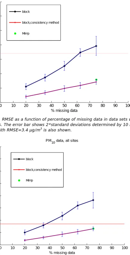
Figure 4A: RMSE as a function of percentage of missing data in data sets with block gaps. The error bar shows 2*standard deviations determined by 10 runs.

The line with RMSE=3.4 µg/m3_{is also shown.}

Figure 4B: RSD as a function of percentage of missing data in data sets with block gaps. The error bar shows 2*standard deviations determined by 10 runs. The line with RSD=0.085 is also shown

0 10 20 30 40 50 60 70 80 90 100 0 1 2 3 4 5 6 7 RM S E % missing data

PM₁₀ data, all sites

block block,consistency method Mimp 0 10 20 30 40 50 60 70 80 90 100 0 0.05 0.1 0.15 0.2 0.25 0.3 0.35 0.4 RS D % missing data

PM₁₀ data, all sites

block

block,consistency method

(29)

Figure 5: yearly concentrations calculated by four individual solutions of the Mimptool. Large deviation between gap-filled data and original data is found at site 553, an industrial site at Wijk aan Zee.

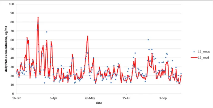
As an example figure 6 shows daily concentrations of PM10 at station 12 (van Diemenstraat) in Amsterdam. The gap-filling was performed by a data set with 75% block gaps. The figure shows that gap-filled data follows measured data quite well.

Figure 6: Gap-filled and measured daily PM10 concentration at Van Diemenstraat in Amsterdam. The measured data block of the plot was (of course) not included in the data set used to calculate the gap filled data.

15 20 25 30 35 40 15 20 25 30 35 40 gap-fi lle d y ea rl y c onc ent ra ti on

original yearly concentration

(30)

5.2 Data set of rural sites

Because the effect of measurements type sites on PM10 concentration is

much less pronouncing, gap-filling of rural sites as a separate data set is only performed with NO2 measurements. This data set consists of 22

sites. Data of 11 sites were kept as such. At 11 sites fictive missing data were created. In tables 6 and 7 average results of 10 runs of the

consistency method are shown for various percentages of missing data. The Mimp tool was only applied in the most difficult test case (a block of 75% missing data) and was performed only once.

Table 6: Results of rural sites.RMSE (in µg/m3_{) of annual average concentrations}

at various percentages of (fictive)missing data: without gap-filling, gap-filled by consistency method and gap-filled by Mimp tool. The green cells show conditions

with RMSE <2 µg/m3

missing data

RMSEgap RMSEfilled

(consistency method) RMSEfilled (Mimp tool) 20 _0.08 _0.14 _1.21 _0.31 35 _0.11 _0.13 _2.40 _0.44 50 _0.14 _0.15 _3.76 _0.69 62.5 _0.18 _0.17 _4.85 _0.83 75 0.25 0.22 5.93 1.12 1.47

Table 7: Results of rural sites.RSD of annual average concentrations at various percentages of (fictive) missing data: without gap-filling, gap-filled by

consistency method and gap-filled by Mimp tool. The green cells show conditions with RSD <0.05

Random gaps Block gaps % fictive missing data RSDgap RSDfilled (consistency method) RSDgap RSDfilled (consistency method) RSDfilled (Mimp tool) 20 _0.004 _0.007 _0.067 _0.016 35 _0.006 _0.007 _0.129 _0.026 50 _0.007 _0.008 _0.201 _0.038 62.5 0.010 0.009 0.276 0.049 75 _0.014 _0.011 _0.343 _{0.073 0.069}

- If missing data are distributed randomly, up to 75% missing data still don’t have significant effect on the annual average

concentration, even when missing data are unfilled.

- When a large block of data is missing, the uncertainty becomes much larger. Gap-filling by consistency method reduces the uncertainty by a factor 5 which is significantly better than when rural data are mixed up with other data. Taking the variations

(31)

between 10 runs into account, up to 50% missing data is still acceptable (Figure 8).

- When rural sites are gap-filled separately the performance of Mimptool is not better than the performance of the consistancy method.

Figure 7: RMSE as a function of percentage of missing data in data sets of rural sites with block gaps. The error bar shows 2*standard deviations determined by

10 runs. The line with RMSE=2 µg/m3_{is also shown.}

Figure 8: RSD as a function of percentage of missing data in data sets of rural

0 10 20 30 40 50 60 70 80 90 100 0 1 2 3 4 5 6 7 RM S E % missing data NO 2 data, R-sites block block,consistency method Mimp 0 10 20 30 40 50 60 70 80 90 100 0 0.05 0.1 0.15 0.2 0.25 0.3 0.35 0.4 RS D % missing data NO 2 data, R-sites block block,consistency method Mimp

(32)

sites with block gaps. The error bar shows 2*standard deviations determined by 10 runs. The line with RSD=0.05 is also shown.

See also annex 3 for yearly concentrations of four individual solutions of the Mimptool as a function of original data.

5.3 Data set of urban background sites

Because the effect of measurements type sites on PM10 concentration is

much less pronouncing, gap-filling of urban background sites as a separate data set is only performed with NO2 measurements. This data

set consists of 19 sites. Data of 10 sites were kept as such. At 9 sites fictive missing data were created. In tables 8 and 9 average results of consistency method are shown. The Mimp tool was only applied in the most difficult test case (a block of 75% missing data) and was

performed only once.

Table 8: Results of urban background sites. RMSE (in µg/m3_{) of annual average}

concentrations at various percentages of (fictive)missing data: without gap-filling, gap-filled by consistency method and gap-filled by Mimp tool. The green

cells show conditions with RMSE <2 µg/m3

missing data

RMSEgap RMSEfilled

(consistency method) RMSEfilled (Mimp tool) 20 _0.09 _0.16 _1.36 _0.50 35 _0.14 _0.16 _2.28 _0.74 50 _0.18 _0.19 _3.66 _1.03 62.5 _0.22 _0.18 _4.91 _1.57 75 _0.30 _0.26 _5.80 _1.76 _1.05

Table 9: Results of urban background sites. RSD of annual average

concentrations at various percentages of (fictive)missing data: without gap-filling, gap-filled by consistency method and gap-filled by Mimp tool. The green cells show conditions with RSD <0.05

Random gaps Block gaps % fictive missing data RSDgap RSDfilled (consistency method) RSDgap RSDfilled (consistency method) RSDfilled (Mimp tool) 20 _0.003 _0.006 _0.050 _0.017 35 _0.005 _0.006 _0.084 _0.025 50 _0.007 _0.007 _0.135 _0.034 62.5 _0.008 _0.006 _0.181 _0.053 75 _0.011 _0.009 _0.215 _0.058 _0.040

(33)

Results in tables 8 and 9 show that:

- When data have a large block gap, the uncertainty becomes much larger. Gap-filling by consistency method reduces the uncertainty by a factor 3 à 4 which is better than when all data are mixed up.

- A percentage missing data of 50% seems to be acceptable (see Figure 10).

- The Mimp tool is only marginally better than the consistency method.

Figure 9: RMSE as a function of percentage of missing data in data sets of urban background sites with block gaps. The error bar shows 2*standard deviations

determined by 10 runs. The line with RMSE=2 µg/m3_{is also shown.}

0 10 20 30 40 50 60 70 80 90 100 0 1 2 3 4 5 6 7 RM S E % missing data NO₂ data, UB-sites block block,consistency method Mimp

(34)

Figure 10: RSD as a function of percentage of missing data in data sets of urban background sites with block gaps. The error bar shows 2*standard deviations determined by 10 runs. The line with RSD=0.05 is also shown.

5.4 Data set of traffic related sites

Because traffic has much less effect on PM10 concentration than on NO2

concentration, gap-filling of traffic related sites as a separate data set is only performed with NO2 measurements. This data set consists of 19

sites. Data of 10 sites were kept as such. At 9 sites fictive missing data were created. In tables 10 and 11 average results of consistency method are shown. The Mimp tool was only applied in the most difficult test case (a block of 75% missing data) and was performed only once.

0 10 20 30 40 50 60 70 80 90 100 0 0.05 0.1 0.15 0.2 0.25 0.3 0.35 0.4 RS D % missing data NO₂ data, UB-sites block block,consistency method Mimp

(35)

Table 10: Results of traffic related sites.RMSE (in µg/m3_{) of annual average}

concentrations at various percentages of (fictive)missing data: without gap-filling, gap-filled by consistency method and gap-filled by Mimp tool. The green

cells show conditions with RMSE <2 µg/m3

missing data

RMSEgap RMSEfilled

(consistency method) RMSEfilled (Mimp tool) 20 _0.12 _0.17 _1.12 _0.58 35 _0.18 _0.20 _1.98 _0.85 50 _0.24 _0.22 _3.04 _1.40 62.5 _0.28 _0.25 _3.37 _1.70 75 _0.38 _0.28 _4.21 _{2.45 3.02}

Table 11: Results of traffic related sites.RSD of annual average concentrations at various percentages of (fictive)missing data: without gap-filling, gap-filled by consistency method and gap-filled by Mimp tool. The green cells show conditions with RSD <0.05

Random gaps Block gaps % fictive missing data RSDgap RSDfilled (consistency method) RSDgap RSDfilled (consistency method) RSDfilled (Mimp tool) 20 _0.003 _0.004 _0.029 _0.015 35 _0.004 _0.005 _0.052 _0.021 50 _0.006 _0.005 _0.083 _0.035 62.5 _0.007 _0.006 _0.090 _0.040 75 0.009 0.007 0.114 0.064 0.080

- When a large block of data is missed, the uncertainty becomes much larger. Gap-filling by consistency method reduces the uncertainty by a factor 2 which is comparable to the results obtained with consistency method when all data are mixed up. - When missing data are gap-filled by consistency method, a

percentage missing data of 50% is still acceptable (figure 12). - There is no indication that Mimp tool is better than consistency

(36)

Figure 11: RMSE as a function of percentage of missing data in data sets of urban background sites with block gaps. The error bar shows 2*standard

deviations determined by 10 runs. The line with RMSE=2 µg/m3_{is also shown.}

Figure 12: RSD as a function of percentage of missing data in data sets of urban background sites with block gaps. The error bar shows 2*standard deviations determined by 10 runs. The line with RSD=0.05 is also show.

0 10 20 30 40 50 60 70 80 90 100 0 1 2 3 4 5 6 7 RM S E % missing data NO 2 data, S-sites block block,consistency method Mimp 0 10 20 30 40 50 60 70 80 90 100 0 0.05 0.1 0.15 0.2 0.25 0.3 0.35 0.4 RS D % missing data NO₂ data, S-sites block block,consistency method Mimp

(37)

(38)

(39)

6 Effect of missing data periods and site locations

In previous figures average RSD’s of 10 runs are shown. The error bars show variations between these runs, i.e. variations between 10 RSD values which were calculated according to formulas (5) and (6).

Variations between relative deviations of individual monitoring sites (as calculated by formulas (3) and (4)) are larger and an individual relative deviation can lay outside the confidence intervals shown in these figures. The relative deviation (rsd) at a monitoring site, (Cmeas,i

-Cfilled,i)/Cmeas,i and (Cmeas,i-Cgap,i)/Cmeas,i respectively, shows the quality of

data before and after gap-filling at that site. This quality is determined by quality of the gap-filling method but also by the period of missing data and by the site location. The consistency method assumes a correlation of measurements over the Netherlands; however, not all sites have the same degree of correlation. The period of missing data is also an important factor. If the remaining period covers only summer or winter period, the data are less representative and deviation with original data can be larger (larger rsd).

In order to investigate these effects, the results of rural sites are worked out in more details. In figure 13 locations of sites with original data and sites with block gaps are shown.

(40)

Figure 13: rural sites used in this study.

In total, there were 22 rural monitoring sites included in this study: 11 sites had fictive block gaps and 11 sites had original data. The gap-filling were performed 10 times, resulting in 110 yearly concentrations of gap-filled data. The dataset had 35% missing data (a block of more than 4 months). Consequently September would be the last month in which the block gap can start. Because the gaps were determined randomly, the number of gaps started in each month was not equal.

(41)

Table 12 shows results of the gap-filling of 35% missing data. In the last two columns, averages of absolute rsd-values of all block gaps started in each month are shown. In figure 14 the results are visualized.

Table 12: Effect of period of missing data

Start time of block gap

Number of data |rsdgap|,average |rsdfilled|,average

January February March April May June July August Total 14 6 12 11 20 19 14 14 110 0.052 0.067 0.142 0.182 0.169 0.145 0.048 0.071 0.029 0.014 0.017 0.014 0.021 0.022 0.015 0.018

Figure 14: Influence of period of missing data on the quality of remaining data and that of gap-filled data. Starting month of the block gaps is shown on the x-axis.

Figure 14 shows strong effect of period of missing data on the quality of remaining data. If the block gap starts in January/February or in

July/August, the remaining data still cover both summer and winter periods and the data are still more or less representative. However if the gap starts in the summer period, the remaining data consist only data of winter period and the difference between these data and the original data becomes significant. The figure shows a very good performance of the consistency method: after gap-filling the deviation is reduced strongly and the effect of missing data period is no longer visible.

A similar analysis was performed to determine the impact of site location on the quality of gap-filled data. The results are shown in table 13 and figure 15. 0,000 0,020 0,040 0,060 0,080 0,100 0,120 0,140 0,160 0,180 0,200

Jan Feb Mar Apr May June July Aug

abs(rsd)

abs(rsd_gaps) abs(rsd_gap‐filled)

(42)

Table 13: Effect of site location

Site nr. Number of data |rsdgap|,average |rsdfilled|,average

131 227 235 411 444 565 633 722 807 918 934 Total 10 10 10 10 10 10 10 10 10 10 10 110 0.100 0.106 0.147 0.107 0.118 0.109 0.102 0.087 0.140 0.092 0.155 0.007 0.008 0.007 0.023 0.009 0.021 0.013 0.024 0.026 0.030 0.050

Figure 15: Effect of site location on the quality of remaining data and that of gap-filled data. Site numbers of monitoring site are shown on the x-axis.

As expected, location of monitoring site does not influence quality of data before gap-filling. However in contrary to period of missing data, location of monitoring site seems to influence the performance of consistency method. Figure 15 shows worse quality of gap-filled data at site 934, a monitoring site in Groningen, in the North of the

Netherlands. The consistency method assumes a correlation between monitoring sites over the Netherlands. This assumption seems to be less valid for Groningen, where there are relatively less monitoring sites than in other areas in the Netherlands.

0,000 0,020 0,040 0,060 0,080 0,100 0,120 0,140 0,160 0,180 131 227 235 411 444 565 633 722 807 918 934 abs(rsd) site nr abs(rsd_gaps) abs(rsd_gap‐filled)

(43)

7 Representativeness of intermittent measurements

In addition to fixed measurements which are required by the Directive, mobile measurements can be used to monitor air quality in typical situations. Such measurements are mostly performed during a short period (a few weeks/months) where after the instruments have to be used at other locations. This study investigates if representative air quality can be obtained by such measurements.

Assumed an instrument is intended to be used at four locations. Obviously several shorter measurement periods will be more

representative than a longer period which only covers part of a year. Too many measurements intervals are not practical, but three periods of a month at each location seem to be feasible. The measurements

scheme is for example as follows:

Table 14: Assumed measurements scheme performed with a mobile instrument. The percentage of “missing data” is 75%

Month scheme 1 scheme 2 scheme 3 scheme 4 January February March April May June July Augustus September October November December X X X X X X X X X X X X X: assumed measured periods

In order to simulate this situation, fictive missing data according to one of the above schemes were created in NO2 data sets. The applied

scheme at each site was chosen randomly. Like in previous evaluations, an equal part of the data set was kept as such to maintain sufficient data in the new data set. Table 15 shows results of the gap-filling of several data sets.

Figure 16 shows that the constraint RMSE<2 µg/m3 _{can be satisfied in all}

gap-filled data sets. However the stricter requirement RSD<0.05 can not be satisfied by all data sets (Figure 17).

Figures 16 and 17 show effect of the pattern of missing data. Compare with a data set with one large block missing data, the data set with 3 small blocks missing data has already much smaller deviations and the effect of gap-filling is quite small.

(44)

Table 15: Results of gap-filling of various sites types. The green cells show

conditions with RMSE <2 µg/m3_{or RSD <0.05}

Sites type

RMSEgap RMSEfilled

(consistency method) RSDgap RSDfilled (consistency method) All sites 1.427 1.075 0.056 0.036 R-sites 1.151 0.618 0.072 0.041 UB-sites 1.533 1.155 0.056 0.044 S-sites 1.562 1.258 0.040 0.033

Figure 16: Effect of the pattern of missing data on RMSE. Data sets with more small blocks of missing data have much lower RMSE and the effect of gap-filling is less pronounced. The error bar shows 2*standard deviations determined by 10

runs. The line with RMSE=2 µg/m3_{is also shown.}

all sites R UB S 0 1 2 3 4 5 6 7 RM S E data set

NO₂ data, 3 blocks vs 1 block

3 blocks

3 blocks,gap-filled

1 block

(45)

Figure 17: Effect of the pattern of missing data on RSD. Data sets with more small blocks of missing data have much lower RSD and the effect of gap-filling is less pronounced. The error bar shows 2*standard deviations determined by 10 runs. The line with RSD=0.05 is also shown.

The same gap-filling procedure was also applied to a second intermittent measurements scheme with less missing data. In this scheme it was assumed that an instrument is used for monitoring at 3 locations. The measurements scheme is as follows:

Table 16: Intermittent measurements scheme corresponding to 66% missing data

Month scheme 1 scheme 2 scheme 3 January February March April May June July Augustus September October November December X X X X X X X X X X X X

The results of the gap-filling are shown in table 17 and Figures 18 and 19. all sites R UB S 0 0.05 0.1 0.15 0.2 0.25 0.3 0.35 0.4 RS D data set NO

2 data, 3 blocks vs 1 block

3 blocks

3 blocks,gap-filled

1 block

(46)

Table 17: Results of gap-filling of various sites types for intermittent

measurements with 66% missing data . The green cells show conditions with

RMSE <2 µg/m3_{or RSD <0.05}

Sites type

RMSEgap RMSEfilled

(consistency method) RSDgap RSDfilled (consistency method) All sites 1.132 0.726 0.048 0.025 R-sites 1.114 0.322 0.065 0.018 UB-sites 1.026 0.610 0.039 0.022 S-sites 1.316 0.869 0.032 0.021

Figure 18: Effect of the pattern of missing data on RMSE. Data sets with more small blocks of missing data have much lower RMSE and the effect of gap-filling is less pronounced. The error bar shows 2*standard deviations determined by 10

runs. The line with RMSE=2 µg/m3_{is also shown.}

all sites R UB S 0 1 2 3 4 5 6 7 RM S E data set

NO₂ data, 4 blocks vs 1 block

4 blocks

4 blocks,gap-filled

1 block

(47)

Figure 19: Effect of the pattern of missing data on RSD. Data sets with more small blocks of missing data have much lower RSD and the effect of gap-filling is less pronounced. The error bar shows 2*standard deviations determined by 10 runs. The line with RSD=0.05 is also shown.

Table 17 and figures 18&19 show that after gap-filling the constraint RSD<0.05 can be fulfilled well by all data sets. From these results we can conclude that 4 months measurements according to the scheme in table 16 will give representative yearly concentration.

all sites R UB S 0 0.05 0.1 0.15 0.2 0.25 0.3 0.35 0.4 RS D data set NO

2 data, 4 blocks vs 1 block

4 blocks

4 blocks,gap-filled

1 block

(48)

(49)

8 Conclusions

 If missing data are distributed randomly, even when ¾ of data are missing, the yearly average concentration obtained by remaining data is still representative. However, in real situations missing data are mostly not totally random. Small blocks of missing data which are randomly distributed are more realistic.  Block of missing data deteriorates the representative of data and

gap-filling is necessary. The quality of remaining data depends on the percentage and on the period of missing data. If data are gap-filled by the consistency method and if the percentage of missing data is less than 35%, the uncertainty of gap-filled data comply with the requirement for EU reporting(max. 15%),

provided that there are sufficient sites with data to be used in the gap-filling (at least an equal number of sites with data must be available).

 In the case of pariculate matter (PM10), even datasets from which

75% of the data is missing can still comply with the required maximum uncertainty of 25%.

 The consistency method assumes a correlation between sites over the Netherlands. This assumption is less valid for sites in Groningen, resulting in relatively bad quality of gap-filled data at this location.

 If data of all sites are gap-filled in one gap-filling, the Mimp tool gives for the NO2 data set better results than the consistency

method (deviation is reduced by a factor 2). This is due to the PCA technique which is included in the Mimptool, making it possible to recognize pattern in the data. When data of each type (rural, urban background, traffic related) are gap-filled

separately, the Mimp tool does not perform better than the (simpler) consistency method.

 When mobile equipments are used to monitor air quality, monthly intermittent measurement periods corresponding to 33% data recovery should be enough to get representative yearly concentration.

(50)

(51)

9 References

AQUILA, The Reporting of Measurement Uncertainties for Regulated Gaseous Air Pollutants and for Particulate Matter and its Constituents in Ambient Air, in Conformance with Directives 2008/50/EC and

2004/107/EC,N256

Geman, S., and D. Geman. 1984. Stochastic Relaxation, Gibbs Distributions, and the Bayesian Restoration of Images. IEEE Transactions on Pattern Analysis and

Machine Intelligence 6721-41.

Hoogerbrugge R. and A.K.D. Liem, How to handle non-detects, Organohalogen

Compounds 45 (2000) 13-16.

De Leeuw, AirBase: a valuable tool in air quality assessments at a European and local level, ETC/ACM Technical Paper 2012/4.

Massart D.L., Vandeginste, B.G.M., Buydens, L.M.C., de Jong, S., Lewi, P.J., and

Smeyers-Verbeke, J. Handbook of Chemometrics and Qualimetrics, Elsevier,

Amsterdam (1997).

Mooibroek, D., Berkhout, J.P.J., Hoogerbrugge. R. (2013) Jaaroverzicht Luchtkwaliteit 2012. RIVM rapport 680704023/2013. Rijksinstituut voor Volksgezondheid en Milieu, Bilthoven. [Dutch].

Mooibroek, D., Vonk,J.,Velders,G.J.M.,Hafkenscheid,T.L., J.P.J.,

Hoogerbrugge. R. (2013) PM2.5 Average Exposure Index 2009-2011 in

the Netherlands. . RIVM rapport 680704022/2013. Rijksinstituut voor Volksgezondheid en Milieu, Bilthoven.

(52)

(53)

Annex 1: Results of determination of corr value by means of

parallel measurements

Dataset Calculated

corr value 448_493 NO2 data of all S-stations. In half of

dataset (among other stations 448&493) block gaps of 50% were created

-0.45

448_493_unfavourable Dataset consists of NO2 data of 4 stations 448,493,136,937. Data of stations 448 and 493 have block gaps of 50%. The gap-filling is performed at unfavourable conditions because data in Rotterdam were gap-filled by means of measurements in Heerlen and

Groningen

-0.35

14_543 NO2 data of all UB-stations. In half of dataset (among other stations 14&543) block gaps of 50% were created

-0.23

14_543_unfavourable Dataset consists of NO2 data of 4 stations 14,543,241,938. Data of stations 14 and 543 have block gaps of 50%. The gap-filling is performed at unfavourable conditions because data in Amsterdam were gap-filled by means of measurements in Breda and Groningen

0.11

14_543_PM PM10 data of all stations. In half of dataset (among other stations 14&543) block gaps of 50% were created

(54)

(55)

Annex 2: sites used in this study (X: site with fictive missing

data)

All sites, NO2 3 X GGD Amsterdam, Nieuwendammerdijk 12 X GGD Amsterdam,Van Diemenstraat 17 X GGD Amsterdam,Stadhouderskade

20 X GGD Amsterdam,Jan van Galenstraat 22 X GGD Amsterdam, Sportpark Ook Meer

131 X Vredepeel - Vredeweg 136 X Heerlen - Looierstraat 227 X Budel - Toom 235 X Huijbergen - Vennekenstraat 237 X Eindhoven - Noordbrabantlaan 247 X Veldhoven-Europalaan

404 X Den Haag - Rebecquestraat 418 X Rotterdam - Schiedamsevest 437 X Westmaas - Groeneweg 444 X De Zilk - Vogelaarsdreef 448 X Rotterdam - Bentinckplein 485 X DCMR,Hoogvliet-Leemkuil 487 X DCMR,Pleinweg-Pleinweg 489 X DCMR,Ridderkerk-Hogeweg 493 X DCMR,Statenweg-Statenweg 495 X DCMR,Maassluis-Kwartellaan 537 X Haarlem - Amsterdamsevaart 565 X PNH, Oude Meer

633 X Zegveld - Oude Meije

639 X Utrecht - Constant Erzeijstraat

703 X HAMS, Amsterdam-Spaarnwoude 738 X Wekerom - Riemterdijk 742 X Nijmegen - Ruyterstraat 818 X Barsbeek - De Veenen 929 X Valthermond - Noorderdiep 937 X Groningen - Europaweg 2 GGD Amsterdam,Haarlemmerweg 7 GGD Amsterdam,Einsteinweg 14 Vondelpark

19 GGD Amsterdam, Oude Schans

21 GGD Amsterdam, Kantershof

107 Posterholt - Vlodropperweg

133 Wijnandsrade - Opfergeltstraat

137 Heerlen - Deken Nicolayestraat

230 Biest Houtakker - Biestsestraat 236 Eindhoven - Genovevalaan

241 Breda - Bastenakenstraat

301 Zierikzee - Lange Slikweg

411 Schipluiden - Groeneveld

433 Vlaardingen - Floreslaan

442 Dordrecht - Bamendaweg

445 Den Haag - Amsterdamse Veerkade

483 DCMR,Botlek (A15)-Botlektunnel 486 DCMR,Pernis-Soetemanweg 488 DCMR,Zwartewaalstraat-Zwartewaalstraat 491 DCMR,Overschie-Oostsidelinge 494 DCMR,Schiedam-Alhpons Ariensstraat 520 Amsterdam - Florapark 538 Wieringerwerf - Medemblikkerweg 631 Biddinghuizen - Hoekwantweg

636 Utrecht - Kardinaal De Jongweg

701 ZNSTD, Zaandam

722 Eibergen - Lintveldseweg

(56)

807 Hellendoorn - Luttenbergerweg

918 Balk - Trophornsterweg

934 Kollumerwaard - Hooge Zuidwal

938 Groningen - Nijensteinheerd R-sites, NO2 131 X Vredepeel - Vredeweg 227 X Budel - Toom 235 X Huijbergen - Vennekenstraat 411 X Schipluiden - Groeneveld 444 X De Zilk - Vogelaarsdreef 565 X PNH, Oude Meer

633 X Zegveld - Oude Meije 722 X Eibergen - Lintveldseweg

807 X Hellendoorn - Luttenbergerweg 918 X Balk - Trophornsterweg

934 X Kollumerwaard - Hooge Zuidwal 107 Posterholt - Vlodropperweg

133 Wijnandsrade - Opfergeltstraat 230 Biest Houtakker - Biestsestraat

301 Zierikzee - Lange Slikweg 437 Westmaas - Groeneweg 538 Wieringerwerf - Medemblikkerweg 631 Biddinghuizen - Hoekwantweg 703 HAMS, Amsterdam-Spaarnwoude 738 Wekerom - Riemterdijk 818 Barsbeek - De Veenen 929 Valthermond - Noorderdiep

Urban background sites, NO2

14 X Vondelpark

21 X GGD Amsterdam, Kantershof

137 X Heerlen - Deken Nicolayestraat

247 X Veldhoven-Europalaan 418 X Rotterdam - Schiedamsevest 485 X DCMR,Hoogvliet-Leemkuil 494 X DCMR,Schiedam-Alhpons Ariensstraat 520 X Amsterdam - Florapark 742 X Nijmegen - Ruyterstraat 3 GGD Amsterdam, Nieuwendammerdijk

19 GGD Amsterdam, Oude Schans

22 GGD Amsterdam, Sportpark Ook Meer

241 Breda - Bastenakenstraat

404 Den Haag - Rebecquestraat

442 Dordrecht - Bamendaweg

488 DCMR,Zwartewaalstraat-Zwartewaalstraat

495 DCMR,Maassluis-Kwartellaan

701 ZNSTD, Zaandam

938 Groningen - Nijensteinheerd

Traffic related (S) sites, NO2

7 X GGD Amsterdam,Einsteinweg

17 X GGD Amsterdam,Stadhouderskade

136 X Heerlen - Looierstraat

237 X Eindhoven - Noordbrabantlaan

445 X Den Haag - Amsterdamse Veerkade

483 X DCMR,Botlek (A15)-Botlektunnel

487 X DCMR,Pleinweg-Pleinweg

491 X DCMR,Overschie-Oostsidelinge

537 X Haarlem - Amsterdamsevaart

639 X Utrecht - Constant Erzeijstraat

937 X Groningen - Europaweg

2 GGD Amsterdam,Haarlemmerweg

12 GGD Amsterdam,Van Diemenstraat

(57)

236 Eindhoven - Genovevalaan 433 Vlaardingen - Floreslaan 448 Rotterdam - Bentinckplein 486 DCMR,Pernis-Soetemanweg 489 DCMR,Ridderkerk-Hogeweg 493 DCMR,Statenweg-Statenweg

636 Utrecht - Kardinaal De Jongweg 741 Nijmegen - Graafseweg

All sites, PM10

12 X GGD Amsterdam,Van Diemenstraat 16 X GGD Amsterdam,Westerpark 20 X GGD Amsterdam,Jan van Galenstraat 133 X Wijnandsrade - Opfergeltstraat 137 X Heerlen - Deken Nicolayestraat 235 X Huijbergen - Vennekenstraat 237 X Eindhoven - Noordbrabantlaan 241 X Breda - Bastenakenstraat 245 X Moerdijk-Julianastraat 247 X Veldhoven-Europalaan 319 X Nieuwdorp-Coudorp 418 X Rotterdam - Schiedamsevest 433 X Vlaardingen - Floreslaan 442 X Dordrecht - Bamendaweg 445 X Den Haag - Amsterdamse Veerkade 447 X Leiden - Willem de Zwijgerlaan 482 X DCMR,Markweg-Markweg 487 X DCMR,Pleinweg-Pleinweg 489 X DCMR,Ridderkerk-Hogeweg 493 X DCMR,Statenweg-Statenweg 495 X DCMR,Maassluis-Kwartellaan 520 X Amsterdam - Florapark 538 X Wieringerwerf - Medemblikkerweg 545 X Amsterdam - A10 west

547 X Hilversum - J. Gerardtsweg 549 X Laren - Jagerspad 553 X PNH, Wijk aan Zee 561 X PNH, Badhoevedorp 565 X PNH, Oude Meer 572 X PNH, Staalstraat 633 X Zegveld - Oude Meije

639 X Utrecht - Constant Erzeijstraat 701 X ZNSTD, Zaandam 704 X HAMS Hoogtij 728 X Apeldoorn - Stationstraat 741 X Nijmegen - Graafseweg 807 X Hellendoorn - Luttenbergerweg 918 X Balk - Trophornsterweg

934 X Kollumerwaard - Hooge Zuidwal 7 GGD Amsterdam,Einsteinweg

14 Vondelpark

17 GGD Amsterdam,Stadhouderskade 131 Vredepeel - Vredeweg

136 Heerlen - Looierstraat 230 Biest Houtakker - Biestsestraat 236 Eindhoven - Genovevalaan 240 Breda - Tilburgseweg

244 De Rips-Klotterpeellaan 246 Fijnaart-Zwingelspaansedijk 318 Philippine - Stelleweg

404 Den Haag - Rebecquestraat 432 Hoek van Holland-Berghaven 437 Westmaas - Groeneweg 444 De Zilk - Vogelaarsdreef 446 Den Haag - Bleriotlaan 448 Rotterdam - Bentinckplein 485 DCMR,Hoogvliet-Leemkuil

(58)

488 DCMR,Zwartewaalstraat-Zwartewaalstraat 491 DCMR,Overschie-Oostsidelinge 494 DCMR,Schiedam-Alhpons Ariensstraat 496 DCMR,Berghaven-Berghaven 537 Haarlem - Amsterdamsevaart 543 Amsterdam - Overtoom 546 Zaanstad-Hemkade 548 Bussum - Ceintuurbaan 551 PNH, IJmuiden 556 PNH, De Rijp 564 PNH, Hoofddorp 570 PNH, Beverwijk-West 631 Biddinghuizen - Hoekwantweg 636 Utrecht - Kardinaal De Jongweg 641 Breukelen - Snelweg 703 HAMS, Amsterdam-Spaarnwoude 722 Eibergen - Lintveldseweg 738 Wekerom - Riemterdijk 743 Kootwijkerbroek - Drieenhuizerweg 818 Barsbeek - De Veenen 929 Valthermond - Noorderdiep 937 Groningen - Europaweg

(59)

Annex 3: yearly concentrations calculated by four individual

solutions of the Mimptool

10 15 20 25 30 35 40 45 50 10 15 20 25 30 35 40 45 50 ga p-fi ll ed y e arl y c on c en tr at ion

original yearly concentration NO₂ data, R-sites 15 20 25 30 35 40 45 50 15 20 25 30 35 40 45 50 gap-f ill ed y ea rl y c onc ent rat ion

original yearly concentration NO₂ data, UB-sites

(60)

25 30 35 40 45 50 55 60 25 30 35 40 45 50 55 60 gap-fi ll ed y ear ly c onc ent rat ion

original yearly concentration NO

(61)

Methods used to compensate for the effect of missing data in air quality measurements