FINAL EVALUATION REPORT OF
CLIMATE DIALOGUE
Marcel Crok, Rob van Dorland, Bart Strengers, Eleftheria
Vasileiadou, Bart Verheggen
Contents
EXECUTIVE SUMMARY
4
1. INTRODUCTION
6
2. CLIMATE DIALOGUES
7
2.1. The melting of the Arctic Sea ice 8
2.2. Long term persistence and trend significance 11
2.3. Are regional models ready for prime time? 14
2.4. The (missing) tropical hotspot 17
2.5. Climate Sensitivity and Transient Climate Response 20
2.6. What will happen during a new Maunder Minimum? 24
3. DESCRIPTION OF CLIMATE DIALOGUE
26
3.1. Approach 26
3.2. Organization 27
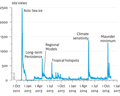
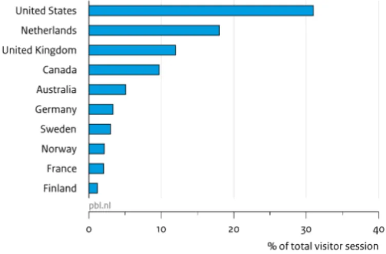
3.3. Audience and blog activity 29
4. LESSONS LEARNT
32
4.1. Internal disagreements 32 4.2. Criticism 33 4.3. Enlisting participants 34 4.4. Time delays 35 4.5. Writing summaries 35 4.6. Blog dynamics 364.7. Lack of institutional support 36
5. FUTURE PLANS
38
Executive Summary
The Climate Dialogue weblog has been a climate change communication project, following a request by the Dutch Parliament, which asked the Dutch Government ‘to also involve climate sceptics in future studies on climate change’.
Climate Dialogue was set up by the Royal
Netherlands Meteorological Institute (KNMI), the Netherlands Environmental Assessment
Agency (PBL), and Dutch science journalist Marcel Crok.
This report, commissioned by the Ministry of Infrastructure and the Environment, constitutes the final evaluation of the Climate Dialogue project.Climate Dialogue was a moderated blog on controversial climate science topics introducing a combination of several novel elements: a) bringing together scientists with conflicting viewpoints; b) strict moderation of the discussion; and c) compilation of executive and extended summaries of the discussions, approved by the participating scientists regarding their statements. Following the ministry request, at least one of the participating scientists was someone perceived to be a climate sceptic. The discussions were technical in nature, and, as a result, the audience of the blog was quite small and specialised.
The Climate Dialogue project operated for slightly more than two years, conducting six dialogues on the natural science of climate change in a polite atmosphere, generating a substantial amount of scientific content, with 20 participating expert scientists, many of them leading in their respective fields. Climate Dialogue also suffered some management problems, and faced criticism from different directions.
The main lessons learnt from this project are:
• The experiment has shown there is potential for a blog such as Climate Dialogue in the polarised landscape of climate change science communication, bringing together scientists with different viewpoints.
• To some extent, the dialogues made clear what the participants agreed on, what they disagreed on and why they disagreed. For example, different views were related to different definitions, disciplines (e.g. focus on statistics vs physics), methods, models and data that scientists favour. In the background, differences in frames probably played a role as well, but these were not explicitly discussed.
• Participating scientists in general were positive about the experience. The friendly and constructive environment in which the dialogues took place probably played a role in that appraisal.
• It was more difficult to attract mainstream climate scientists than sceptical climate scientists. One important reason was what is sometimes called ‘false balance’, i.e. the perception that the format of specifically inviting sceptical scientists to the dialogue gives them more ‘weight’ than they have in the broader scientific community, and as such provides a skewed view of the scientific debate.
• A project of this kind should be operated preferably by an international team including people that have a well-respected position amongst mainstream climate scientists.
• Institutional support from either well-known international climate institutes or professional bodies, such as EGU, AGU, AMS and EMS, would help to ensure continuity of Climate Dialogue and participation by mainstream climate scientists. • To motivate expert participation it would be helpful if climate dialogues lead to a peer
With respect to the future of the Climate Dialogue project, even though some effort has been made to continue in a similar or adapted format under different organisational support, to date there is no clear future trajectory for the Climate Dialogue project.
1. Introduction
The Climate Dialogue weblog, funded by the Dutch Ministry of Infrastructure and the Environment (IenM), started in September 2012, following a request by the Dutch Parliament1 to the government ‘to also involve climate sceptics in future studies on climate
change’. The motion reflected the political response in The Netherlands to mistakes identified in the IPCC report AR4 (Working group II), as well as the InterAcademy Council review of IPCC procedures.
The blog proved to be a controversial climate change communication project, as it has been both praised as a worthwhile experience of ‘scientific mediation’ by Judith Curry and criticised as presenting ‘science […] like a talk-show debate, giving equal weight to all opinions and “beliefs”’ by James Hansen. The intensity of the criticism, apparent on the comments posted on influential blogs2, indicates how polarised the climate change debate is,
not only in the public domain, but also in the climate science community itself.
The first Climate Dialogue on Arctic Sea Ice was launched on 9 November 2012. On 31 December 2014, after more than two years of operation, the last dialogue on Sun activity formally came to an end. There are three distinct phases in the project: 1) September 2012-September 2013; 2) October 2013 – December 2013; and 3) January 2014-December 2014. In the first phase the website was built and 4 dialogues were organised. The second phase was characterised by inactivity as the funding had run out. Then in December 2013, the Parliament decided to finance the project for one more and final year, to properly round off the project and/or to find another source of funding for the project. During this third phase, two more dialogues were organised and summaries of the phase-one-dialogues were finalised.
The current report evaluates the Climate Dialogue project in the following five chapters: 1. Summary of the six Climate Dialogues, based on the documentation on each
dialogue, available at www.climatedialogue.org.
2. Overview of the project’s approach, organisation, and audience. 3. Lessons learnt in the process.
4. Assessment of the future prospects of the concept behind Climate Dialogue. 5. Outline of a co-authored paper on the lessons learnt from Climate Dialogue.
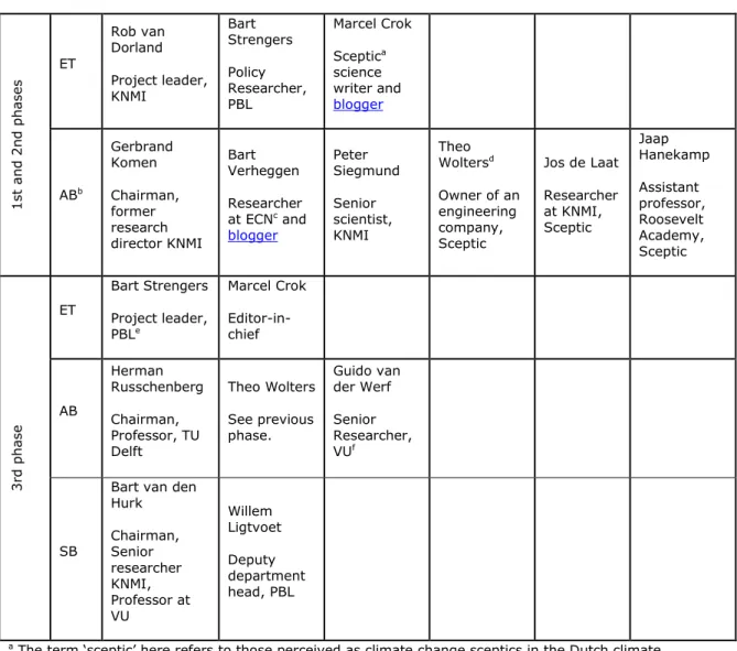
This evaluation was coordinated by Eleftheria Vasileiadou, Assistant Professor at the School of Innovation Sciences, Eindhoven University of Technology. The writing team included Bart Strengers (Project Leader), Marcel Crok (Editor in Chief), Bart Verheggen (member of the Advisory Board during the first phase and PBL advisor during the third), and Rob van Dorland (Project Leader of the first phase).
Information used in the process evaluation is based on input from all co-authors, as well as on material from interviews with (a) individuals involved in the organisation of Climate Dialogue; (b) scientists participating in the discussions; and (c) a limited number of stakeholders around the Climate Dialogue project. The interviews were conducted taking all ethical considerations into account, ensuring full anonymity for the interviewees, including a signed informed consent form. The 24 interviews were conducted in November 2013; thirteen interviews in person (face-to-face or via Skype), and eleven via email. The interviews included all active members of the project (Editorial Team and Advisory Board) at that time, and nine of the twelve participating scientists. This material was analysed in the
1 Dutch House of Representatives, documents 31 793, no. 54 (in Dutch) 2 Such as Realclimate and Wattsupwiththat
interim evaluation report, published in December 2013. Finally, we also used basic weblog visitor statistics, together with public data from other prominent climate blogs.
2. Climate Dialogues
In total six topics were discussed at the Climate Dialogue website. The sixth and last discussion is still going on at the time this evaluation was conducted. In all dialogues the invited scientists were influential and well-known in their respective fields (see Table 1).
Topic Discussants
Melting of Arctic sea ice
(November 2012)
Walt Meier (Research Scientist at NASA, USA)
Judith Curry (Professor of Earth and Atmospheric sciences, Georgia Institute of
Technology, USA), S
Ron Lindsay (Senior Principal Physicist, University of Washington, USA)
Long term persistence and trend significance (April 2013)
Rasmus Benestad (Senior Scientist, Norwegian Meteorological Institute, Norway) Demetris Koutsoyiannis (Professor of Hydrology and Analysis of Hydrosystems
University of Athens, Greece), S
Armin Bunde (Professor of Theoretical Physics, University of Giessen, Germany)
Are regional models ready for prime time? (May 2013)
Bart van den Hurk (Senior Researcher Global Climate, Royal Netherlands
Meteorological Institute)
Jason Evans (Associate Professor Regional Climate and Water resources,
University of Newcastle, Australia)
Roger Pielke Sr. (Senior Research Scientist/ Emeritus Professor of Atmospheric
science, University of Colorado in Boulder, USA), S The (missing)
tropical hotspot (July 2013)
Carl Mears (Senior Research scientist Remote Sensing Systems, USA)
Steven Sherwood (Professor of Physical Meteorology and Atmospheric Climate
Dynamics, the University of New South Wales, Australia)
John Christy (Distinguished Professor of Atmospheric Science, University of
Alabama in Huntsville, USA), S Climate sensitivity
(May 2014)
James Annan (Independent climate scientist, Blue Skies Research, the UK) John Fasullo (Project Scientist in the Climate Analysis Section at National Center
for Atmospheric Research and a Research Associate, the University of Colorado, USA)
Nic Lewis (Independent climate scientist, the UK), S
New Maunder Minimuma
(October 2014, not finished as of February 2015)
Mike Lockwood (Professor of Space Environment Physics, University of Reading,
the UK)
Nicola Scafetta (Research scientist at the Active Cavity Radiometer Solar
Irradiance Monitor Lab group and an adjunct assistant professor in the Physics department, Duke University, USA), S
Jan-Erik Solheim (Professor Emeritus at the Institute for Theoretical
Astrophysics, University of Oslo, Norway), S
Ilya Usoskin (Professor of Physics, University of Oulu, Finland)
José Vaquero (Lecturer in Earth Physics (Centro Universitario de Mérida,
University of Extremadura, Spain)
Table 1. Overview of topics and experts that participated in the dialogues (S=Perceived as
2.1. The melting of the Arctic Sea ice
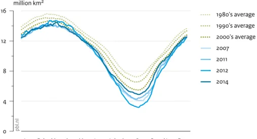
The decline of Arctic sea ice has been one of the most striking changes of the Earth’s climate in the past three decades. In September 2012 the sea ice extent reached a new record low after an earlier record in 2007. The melting is especially strong at the end of summer, during which ice extent has decreased by ~50% compared to the average values in the 1980’s (see Figure 1).
Figure 1. Arctic sea ice extent in the period 1979-2014. Source: Arctic Sea-ice Monitor.
Sea ice volume, i.e. extent times thickness, has decreased even more, with the monthly averaged ice volume for September 2012 of 3,400 km3, which is 72% lower than the mean
over the period since 1979. If these trends continue the Arctic will be ice free in the summer in a few years to decades. The decrease in Arctic sea ice has occurred faster than climate models predicted.
A key question of course is how much of the melting of the Arctic sea ice is caused by anthropogenic activity, chiefly the increase in greenhouse gases. All three participants agreed that at least some of the melting is due to global warming, both natural and anthropogenic. This agreement relieved some of the pressure in the discussion and probably helped to have a friendly and constructive, but not very sharp first Climate Dialogue.
All three participants have published extensively about Arctic sea ice. It wasn’t easy to find a “sceptical” voice for this dialogue. In the blogosphere “sceptics” are eager to point out that the melting of the Arctic sea ice is a natural phenomenon. However it’s not easy to find publishing climate scientists claiming just that. Curry is one of the most “sceptical” voices of those scientists who have published in the literature about Arctic sea ice. Meier and Lindsay can be regarded as “mainstream”. We also invited Peter Wadhams, a British researcher who has claimed the Arctic could be ice free within a few years already, based on linear extrapolation of recent trends. Wadhams initially agreed to participate but later he declined due to time constraints.
The Climate Dialogue
There was full agreement on the basic facts that both sea ice extent and volume have decreased considerably over the last 30 years.
The participants disagreed slightly on how unprecedented the current decline in sea ice is. Lindsay and Meier had more confidence that the current decline is unprecedented within a historical context. Curry argued that data from before 1979, when satellite observation of the sea ice started, are not reliable enough to obtain a good understanding of the state of Arctic sea ice in the past. The participants agreed that during the summers in the Holocene Thermal Maximum (around 8000 years ago) the Arctic likely was ice free or near ice free, as well. At that time, temperatures in the Arctic were similar to or even higher than those of today.
The participants also agreed that the start of the decline in Arctic Sea Ice in the late 1980s coincided with a shift in the so-called Arctic Oscillation. A positive Arctic Oscillation, i.e. high sea level pressures in the Arctic area, especially in winter, pushed older and thicker ice out of the Arctic through the Fram Strait, which is the sea between Greenland and Svalbard. When the Arctic Oscillation went back to normal however, the decline in sea ice continued. Meier and Lindsay conclude from this that natural oscillations probably played a minor role in the continuing decline of sea ice. Moreover simulations with climate models suggest that the Atlantic Multidecadal Oscillation (AMO), i.e. multidecadal periods of warmer and cooler than average temperatures in the Atlantic Ocean, might have contributed between 5% and 30% to the melting. This strengthens Meier’s and Lindsay’s belief that most of the melt is the result of global warming.
This also generated the greatest disagreement within the dialogue. Meier and Lindsay think that climate models simulate natural variability reasonably well, but Curry believes that they underestimate this variability. Curry is unimpressed by how well climate models simulate the Arctic climate and notes that the high attribution of the melt to global warming, both anthropogenic and natural, depends on these models.
Nevertheless Curry agreed that at least 30% of the melt would be the result of anthropogenic global warming. Her upper limit of 70% influence of greenhouse gases on the melt, however, is lower than the 95% upper limit that Meier and Lindsay think is reasonable (See Table 2).
Meier Curry Lindsay
What is your preferred range w.r.t. the contributions of
anthropogenic forcing to the decline in sea ice extent? 50-95% 30-70% 30-95% What is your preferred range w.r.t. the contributions of
anthropogenic forcing to the decline in sea ice volume? 50-95% 30-70% 30-95%
Table 2. How large is the role of anthropogenic global warming?
Curry said she would not know of any publishing climate scientist giving a lower estimate than 30%. Curry proposed a range of 30 to 70% greenhouse gas contribution to the recent decline in sea ice extent. Her best estimate would be 50%. Lindsay agreed with this best estimate of 50% for extent. He added though that sea ice volume is his preferred metric because it shows less year to year variability. For sea ice volume he would go higher, to about 70%.
Later in the discussion all three participants acknowledged there was a great deal of uncertainty when making attribution statements. Meier for example wrote: “There seems to be a lot of wrangling over exactly what fraction of the observed change is attributable to greenhouse gases vs. natural and other human [factors](e.g., black carbon). There is clearly still uncertainty in any estimates and the models and data are not to the point where we can
pin a number with great accuracy. Judith is more on the lower end, rightly pointing out the myriad natural factors. Ron and I tend toward the higher end.”
Future
None of the participants believe that the Arctic will be ice free in the summer within a few years, as some climate scientists, e.g. Wadhams, have claimed in the media. Meier explained that so far the “easy” ice has melted but that now we’re getting to the “more difficult” ice north of Greenland and the Canadian Archipelago. Lindsay is most confident that even on a time scale of one or two decades greenhouse forcing will cause a further decline. Curry emphasized that on this time scale natural fluctuations will dominate the effect of CO2. For
her a reverse of the trend is therefore possible and she didn’t want to speculate when the summer will be ice free. Meier “wholeheartedly” agreed with Curry that decadal prediction of sea ice is going be very difficult. Nevertheless Meier believes it is going to happen somewhere over the period 2030-2050 period while Lindsay uses the longer 2020-2060 period.
None of the participants believe in a tipping point (a point of no return). Lindsay noted that if we magically could turn off the forcing (i.e. get rid of the anthropogenic greenhouse gases) the sea ice would recover rather quickly.
Meier Curry Lindsay
The Arctic could be ice-free in a few years. Very unlikely Very unlikely Very unlikely What is the most likely period that the Arctic will be ice
free for the first time? 2030-2050 X 2020-2060
2.2. Long term persistence and trend significance
Long term persistence (LTP) or long term correlation is a statistical characteristic of how a quantity is changing over time. If the quantity is found to depend on historical values from long ago, it exhibits LTP or long term correlation. Many natural quantities, such as river run-off, have been found to exhibit such long term correlated behavior. Applied to long-term climate records, LTP is present if deviations from the long term mean tend to persist, e.g. warm years are likely to be followed by warm years. In practice, LTP can lead to long lasting anomalies. It is important to realize that this statistical “behavior” is the result of all physical processes in the climate system, internal dynamics and climate forcings, both natural and anthropogenic. This Dialogue focused on the presence of LTP in time series of global mean surface temperature (GMST) and its relevance for the detection of climate change and for the role of internal variability.
The participants in this dialogue were Rasmus Benestad, Armin Bunde and Demetris Koutsoyiannis, the latter two being sceptical of the IPCC positions. Benestad is a climate scientist at the Norwegian Meteorological Institute. He has published on statistical techniques related to climate observations. Bunde is a statistician at the University of Giessen in Germany and has published on long term persistence in proxy observations of global temperature. Koutsoyiannis is a hydrologist at the University of Athens, Greece. He has
published on statistical behavior of hydrological as well as climate observations. The Climate Dialogue
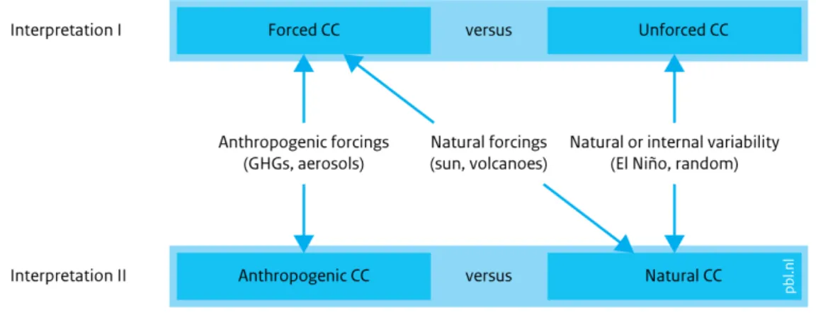
The three discussants agreed that time series of global average temperature indeed exhibit LTP, though they disagreed about its relevance for the detection of a significant warming trend and for the role played by internal variability. This dialogue was hindered by differences in the interpretation of the concept of ‘detection’, which became apparent towards the end of the dialogue. To explain these differences one need to understand ‘forced’ vs ‘unforced’ and ‘anthropogenic’ vs ‘natural’ changes in the climate system (see Figure 2).
Figure 2. Two different interpretations of the definition of detection as used by the
Forced changes in the climate arise from a change in the balance between in- and outgoing radiation at the top of the atmosphere. These forced changes can be either natural, e.g. from changes in the sun or volcanic activity, or anthropogenic, e.g. from changes in atmospheric greenhouse gas or aerosol concentrations (see Figure 2). Unforced changes in the climate refer to natural fluctuations or semi-random processes internal to the climate system. This internal variability usually involves a redistribution of energy among different components of the climate system, for example due to El Niño which causes heat from the ocean to be brought into the atmosphere.
According to IPCC AR5 “Detection of change is defined as the process of demonstrating that climate or a system affected by climate has changed in some defined statistical sense without providing a reason for that change. An identified change is detected in observations if its likelihood of occurrence by chance due to internal variability alone is determined to be small.”
According to Benestad this definition of detection is based on distinguishing the ‘forced’ from the ‘unforced’ components of change. In other words, Benestad took the approach of comparing the observed warming trend with what would be expected from internal variability alone, following Interpretation I. Bunde and Koutsoyiannis reject Interpretation I as they believe the data cannot give us what is called "unforced" or "forced" signals and they do not trust models to be able to do so either. They do believe that the data of a past period incorporate both the effects of natural forcings and internal variability but they do not believe that separation of these two is feasible or even meaningful.
The IPCC definition led to a heated debate. Koutsoyiannis and Bunde interpreted the phrase “in some defined statistical sense without providing a reason for that change” as detection of climate change being only or mainly a matter of statistics and choosing the appropriate statistical model. They argued that LTP is the proper model to describe temperature changes (arising from forced and unforced changes) and mainly discussed statistical methods to retrieve the extent of LTP from temperature records to determine whether the increase in global average temperature in the past 150 years is statistically significant or not. In doing so they followed interpretation II, i.e. they analyzed whether the recent warming is outside the inferred natural range taking into account the extent of LTP as deduced from the same temperature series, which according to Koutsoyiannis corresponds to the LTP over the past 50 million years of Earth’s history. Benestad compares observed warming with the magnitude of internal variability as expected based on climate models, i.e. following interpretation I.
By not distinguishing between the two modes of natural influence (internal variability and natural forcing), Bunde and Koutsoyiannis in effect set a higher bar than used in Interpretation I, for which the observed change only needs to exceed that expected from unforced internal variability.
Presence of Long term persistence
All three invited participants agreed that radiative forcing can introduce LTP and that both forcings and LTP are omnipresent in climate records. Since internal variability is also always present, it follows that the presence of LTP cannot be used to distinguish forced from unforced changes in global average temperature. Therefore, LTP by itself does not provide insight into the causal mechanism of climate change.
According to Bunde “natural forcing plays an important role for LTP and is omnipresent in climate”. Koutsoyiannis agreed that “(changing) forcing can introduce LTP and that forcing is
omnipresent. But LTP can also emerge from the internal dynamics alone” as a result of the irregular and unpredictable changes that take place in the climate. For Benestad LTP or memory is a manifestation of the slow climate response of e.g. the oceans that warm very slowly as the result of changes in the energy balance of the global climate system (i.e. radiative forcing).
Is the observed warming significant?
All participants agreed that the presence of LTP lowers the statistical significance of a trend compared to when only short term correlation is taken into account. According to Bunde and Koutsoyiannis the latter leads to a strong overestimation of the significance of global warming. In their opinion, IPCC wrongly applies Short Term Persistence (STP) models for estimating the significance of the recent warming trend. Benestad agreed that the STP models “may not necessarily be the best” models, but in general statistical models are useless in his opinion when applied to global mean temperature time series, because in this period the data embed both “signal” (forced changes) and “noise” (unforced changes) and LTP or STP or whatever statistical model are meant to describe “the noise” only, when following interpretation I. Moreover, state-of-the-art detection and attribution work as assessed by IPCC does not necessarily rely on the STP concept, but use results from climate models rather than simple STP methods.
In the end, the three participants gave different answers to whether the warming in the past 150 years is significant or not. Benestad was most confident that both the changes in land and sea temperatures are significant. To reach this conclusion he relied on the abovementioned detection and attribution methods. He also applied regression analysis and ranking tests to assess the likelihood for the warming being a result of coincidence. These tests did not take into account potential LTP though.
To Bunde and Koutsoyiannis LTP is the proper model to describe the changes in GMST. In their view, physical knowledge of the climate system is rather irrelevant to establish detection. They disagreed however about whether the current warming is statistically significant, where Bunde answered “yes” except for the global Sea Surface Temperature and
Koutsoyiannis was leaning towards “no”. Bunde argued that, due to LTP, the global average sea surface temperature changes are not significant but the land and global (composite of land and sea surface) temperature changes are. Koutsoyiannis concluded the warming in the past 134 years is not significant - using a stricter level of significance though, namely 99% rather than the more common 95%.
Causes of observed warming
Bunde is more convinced that greenhouse gases have a substantial effect on global temperatures than Koutsoyiannis, although he also said he cannot rule out that the warming is (partly) due to other causes such as the Urban Heat Island effect.
When we asked Koutsoyiannis whether he believes the influence of greenhouse gases is small he answered: “Yes, I believe it is relatively weak, so weak that we cannot conclude with certainty about quantification of causative relationships between greenhouse gas concentrations and temperature changes.”
Benestad on the other hand wrote: “The combination of statistical information and physics knowledge lead to only one plausible explanation for the observed global warming, global mean sea level rise, melting of ice, and accumulation of ocean heat. The explanation is the increased concentrations of greenhouse gases.”
2.3. Are regional models ready for prime time?
Climate models are vital tools for helping us understand long-term changes in the global climate system. Global climate projections for 2050 and 2100 have, amongst other purposes, been used to inform potential mitigation policies, i.e. to get a sense of how the climate system would be expected to evolve in response to different emission scenarios. The next logical step is to use models for adaptation as well, which requires a more regional approach. Stakeholders have an almost insatiable demand for future regional climate projections. These demands are driven by practical considerations related to freshwater resources, ecosystems and water related infrastructure, which are vulnerable to climate change.
Hundreds of studies have been published in the literature presenting regional projections of climate change for 2050 and 2100. The output of such model simulations is then used by the climate impacts community to investigate what potential consequences could be expected in the future, depending on the emission scenario. However several recent studies cast doubt whether global model output is realistic on a regional scale, even in hindcast3 .
The question in this dialogue was whether regional climate models are ready to be used for regional projections? Is the information reliable enough to use for medium to long term adaptation planning? Or should we adopt a different approach?
The following three participants joined this discussion: Bart van den Hurk of KNMI in The Netherlands who is actively involved in the KNMI regional climate scenario’s, Jason Evans from the University of Newcastle, Australia, who is coordinator of Coordinated Regional Climate Downscaling Experiment (CORDEX) and Roger Pielke Sr. who through his research articles and his weblog Climate Science is well known for his outspoken views on climate modelling. For clarity, both Evans and Van den Hurk are actively involved in regional climate scenarios (decades into the future), Pielke is not.
For personal reasons Evans wasn’t able to participate actively in the dialogue after the guest blogs and the first comments were published.
The Climate Dialogue
The key issue in this dialogue was whether regional climate scenarios for 2050 or 2100 are “good” or “reliable” enough to be used for e.g. infrastructural planning decisions on a regional and multidecadal scale. For example should we increase dikes along our rivers if climate projections indicate that extreme rainfall will likely increase in the coming decades? Pielke’s answer to this question is “no”. Pielke wrote that “by presenting the global, regional, and local climate projections as robust (skillful) to the impacts and policy communities we are misleading them on the actual level of our scientific capability.” And also (in his guest blog): “using the global climate model projections, downscaled or not, to provide regional and local impact assessment on multi-decadal time scales is not an effective use of money and other resources.”
3 van Oldenborgh, G. J., Reyes, F. D., Drijfhout, S. S., & Hawkins, E. (2013). Reliability of regional climate model trends. Environmental Research Letters,8(1), 014055.
Anagnostopoulos, G. G., Koutsoyiannis, D., Christofides, A., Efstratiadis, A., & Mamassis, N. (2010). A comparison of local and aggregated climate model outputs with observed data. Hydrological Sciences
Journal–Journal des Sciences Hydrologiques, 55(7), 1094-1110.
Stephens, G. L., L'Ecuyer, T., Forbes, R., Gettlemen, A., Golaz, J. C., Bodas‐Salcedo, A., ... & Haynes, J. (2010). Dreary state of precipitation in global models. Journal of Geophysical Research: Atmospheres
(1984–2012),115(D24).
Bhend, J., & Whetton, P. (2013). Consistency of simulated and observed regional changes in temperature, sea level pressure and precipitation. Climatic change, 118(3-4), 799-810.
Evans has a different opinion as expressed in this comment: “In the end, climate models are our best tools for understanding how the climate system works. As climate scientists, we will continue to use these tools to improve our understanding of the climate system, and use our understanding of the system to improve these tools. Part of this includes exploring the impact of changing levels of greenhouse gases on the climate by creating future climate projections.” And in another comment he wrote: “So RCMs [Regional Climate Models] are not perfect but in many cases are good enough to be useful.” Van den Hurk agreed with Evans by writing in his guest blog that: “RCMs can be of great help, not necessarily by providing reliable predictions, but also by supporting evidence about the salience of planned measures or policies.”
So Evans and Van den Hurk are more positive than Pielke with respect to the central question in the title “Are regional climate models ready for prime time?” All discussants agree that models still have (a lot of) imperfections, also when simulating the past. For Evans and Van den Hurk model projections are nevertheless useful, for Pielke they are useless and he prefers other approaches.
Skill
A returning remark of Pielke was that models need to show “skill” in hindcast before it makes sense to use future projections. Skill is defined by Pielke as “an ability to produce model results for climate variables that are at least as accurate as achieved from reanalyses.” where reanalysis data consists of a combination of observations and model output. This is often necessary to check model output against, because observations alone are not detailed enough to validate the models. Pielke continues: “The skill needs to be tested using hindcast runs against: i) the average climate over a multi-decadal time period and ii) CHANGES in the average climate over this time period.” Pielke claimed models don’t have this skill even back in time, so projecting them to the future makes no sense to him.
Van den Hurk didn’t use this definition of skill. He wrote: “I don’t know how to assess skill of decadal trends, and so do not require models to reproduce the past trends. A measure of skill of predictions thus should be that the observed climate trends fall within the range of an ensemble4 of hindcast predictions.”
So the definition of Pielke is much stricter than that of Van den Hurk. Actually when asked about Pielke’s definition, Van den Hurk agreed that models are not yet up to that task: “For predictions at the decadal time scale, as Roger identifies in his Type 4 application [i.e. climate scenarios], assessment of skill is actually barely possible. Even a perfect model can deviate significantly from past observed trends or changes, just because the physical system allows variability at decadal time scales; the climate and its trend that we’re experiencing is just one of the many climates that we could have had.”
So they disagreed on the operational definition of skill, but as Van den Hurk wrote: “I think we should conclude that we agree on the fact that on shorter (decadal) time scales GCM/RCM [Global Climate Models/Regional Climate Models, red] have shown little regional skill to predict/hindcast observed changes. But that does not necessarily imply that they are useless or have no skill on longer time scales.” and “The purpose of a projection is to depict the possible (plausible) evolution of the system. To my opinion, the process of decision making is not dependent on the (quantitative) predictions provided by climate models, but by the plausibility that the future will bring situations to which the current system is not well adapted.”
Pielke agreed “with the need to assess what is plausible”, but said that the scientific community should be honest about the possibility that “the scenarios that you provide from
4An ensemble is a group of model simulations. This is done to get an idea of the average trend of the models under a given scenario.
the downscaled models may fall outside the range of what actually could occur. If one insists, they could be included, but there should be a disclaimer given to the policymakers that these regional forecasts have not shown skill when tested in a hindcast mode.”
Top down versus bottom up
For Pielke a more robust approach is to use historical, paleo-record and worst case sequences of climate events. “Added to this list can be perturbation scenarios that start with regional reanalysis (e.g. such as by arbitrarily adding a 1C increase in minimum temperature in the winter, a 10 day increase in the growing season, a doubling of major hurricane landfalls on the Florida coast, etc). There is no need to run the multi-decadal global and regional climate projections to achieve these realistic (plausible) scenarios.” Pielke calls his approach the ‘bottom up vulnerability approach’ and contrasts this with the IPCC approach of first generating projections and then using these projections as input for impact models. This is what he would call the top down approach.
On the usefulness of the vulnerability approach Van den Hurk fully agreed with Pielke: “I fully embrace Pielke’s plea for a system analysis that takes the vulnerability of the system as a starting point.” but he also stressed that “from this kind of analyses, frequently the stakeholders are the participants that ask for support from (regional) climate models to illustrate the possible alternative future conditions.” Van den Hurk thus argues that both approaches are complementary.
2.4. The (missing) tropical hotspot
Based on theoretical considerations and simulations with General Circulation Models (GCMs), it is expected that any warming at the surface will be amplified in the upper troposphere. More warming at the surface means more evaporation and more convection. Higher in the troposphere the (extra) water vapour condenses and heat is released. As such this so-called (tropospheric) hot spot is not specific to what caused the warming: any surface warming is expected to be amplified higher up in the atmosphere. Calculations with GCMs show that the lower troposphere warms about 1.2 times faster than the surface. For the tropics, where most of the moisture is, the amplification is larger, about 1.4. Thus the absolute warming trend is also expected to be higher in the troposphere than on the surface. Originally, this amplification effect was dubbed the 'tropical hot spot', but the term is often also used for this absolute trend.
Temperature data sets for the (tropical) troposphere based on weather balloons or so-called radiosondes start in 1958. Data sets based on satellite measurements start in 1979. So, now that we have several decades of data and it can be examined whether the theoretical or model expectations hold up in the observations. The issue became controversial when US scientists John Christy and Roy Spencer started to build their satellite data set in the 1990s5,
because originally this showed no warming at all in the global troposphere. Later, several deficiencies were found and corrected in their data set and a second group of scientists (RSS, Carl Mears and Frank Wentz) also prepared a temperature time series, both of which showed warming of the troposphere.
However, some of the controversy has remained, because both satellite and radiosonde data sets still show (much) less warming than models indicate. John Christy, Fred Singer and others pointed this out in a 2008 article in the International Journal of Climatology6, but this
was criticised in the same issue of the journal by another article co-authored by a large group of climate scientist7. The original article claimed that models and observations differed
significantly. The critique on the article was that the authors had underestimated the uncertainties in both the models and the observations, and that, when taking these uncertainties into account, the ranges for models and observations would overlap. Ergo, models and observations could still be in agreement. The models were not “falsified”.
Steven Sherwood (AUS) and Carl Mears (USA) were co-authors of the article that criticized the article by Christy and Singer. Thus, with Mears, Sherwood and Christy as participants in this Climate Dialogue we had three scientists who are all very familiar with this issue.
The Climate Dialogue Amplification
The introduction article and the questions asked of the participants focused on the amplification aspect of the tropical hot spot, i.e. the fact that warming at the planet's surface should be amplified higher up in the troposphere. The participants agreed that, in theory, one indeed expects this amplification. Also Christy accepted that the tropical hot spot is not a unique fingerprint, which means that any warming influence on the climate – irrespective of the cause – should produce amplified warming aloft.
5 University of Alabama in Huntsville (UAH) satellite temperature dataset
6 Douglass, D. H., Christy, J. R., Pearson, B. D., & Singer, S. F. (2008). A comparison of tropical temperature trends
with model predictions. International Journal of Climatology, 28(13), 1693-1701.
7Santer, B. D., Thorne, P. W., Haimberger, L., Taylor, K. E., Wigley, T. M. L., Lanzante, J. R., ... & Wentz, F. J. (2008).
Consistency of modelled and observed temperature trends in the tropical troposphere. International Journal of Climatology, 28(13), 1703-1722.
If we focus on the amplification, it is really hard to prove that the amplification factors in the models differ significantly from those in the observations. The main reason for this is that you divide tropospheric warming by surface warming; these two numbers are both quite small and this generates huge uncertainties. Sherwood and Mears claimed that the uncertainties were too big to say anything conclusive about this. They were supported in this opinion in the public comments by Ross McKitrick, a well-known sceptic, who has published several papers about the tropical hot spot. However, based on a slightly different selection of the available data sets, Christy claimed that models also show significantly more amplification than the observations. So there was no agreement on this.
Absolute trend in the tropical upper troposphere
The more controversial issue is the fact that models – given the measured increase in greenhouse gases over the past 60 years – simulate an absolute warming trend in the upper tropical troposphere that is significantly greater than shown by the data sets. So, the key term here is not 'amplification' but 'the magnitude of the trend', as also dealt with in the two 2008 articles.
Christy focused much more on this aspect in the debate than Sherwood and Mears did, who preferred to focus on the amplification. However, Sherwood and Mears also made clear that this second aspect of the discussion is actually the most interesting issue.
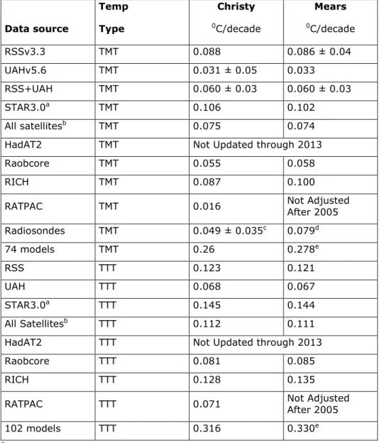
Quite surprisingly – given the heated debate in the past – there was also quite some agreement about the absolute difference in trends between models and observations. During the discussion, sometimes, Mears and Christy mentioned different trends for the same data set. Therefore, we prepared Table 4 to explicitly show these differences. The table shows that observational TMT trends vary between 0.02 and 0.11°C/decade while the models produce trends of 0.26 to 0.28°C/decade. For TTT the observational trends are slightly higher (0.07–0.15°C/decade) and the model trends as well (0.32–0.33°C/decade). During the preparation of this table, Christy and Mears agreed almost completely about the trend numbers in different data sets and they agreed that the absolute trends of models and observations differ significantly. Mears: 'Measured trends in the tropical troposphere are less than all of the modelled trends. This is an important, statistically significant, and substantial difference that needs to be understood.' Sherwood agreed with this conclusion for the satellite period (since 1979) but not for the full period since 1958.
Possible causes
The main topic for discussion now was to understand the causes for the discrepancy between models and observations in the tropical upper troposphere. Here, the participants disagreed, putting forth different hypotheses.
Sherwood thought the data on the troposphere could be wrong. He assumed there has been more cooling in the stratosphere (the layer above the troposphere) than anyone has reckoned. Satellite measurements for the upper troposphere include a signal (less than 10%) from the stratosphere. This stratospheric signal has to be removed to get the upper-tropospheric temperature right. If in reality there is more cooling in the stratosphere than the RSS and UAH groups assume, then this reduces their upper troposphere temperature trend. Sherwood therefore thought that the true upper-tropospheric warming could be stronger than what any group would infer from the satellite data.
Christy, on the other hand, thought the surface data still have a warm bias and overestimate the 'real' warming trend. A (much) smaller surface trend could in theory 'repair' the amplification ratio between the surface and the tropical troposphere. But this would make the differences in the absolute warming trends between models and surface observations even worse. Models would then not only overestimate the warming trend of the tropical upper-troposphere but also at the tropical surface.
Mears thought of a combination of natural variability (which is not well-simulated by an ensemble of models), heat going into the deep ocean, solar changes, volcanic aerosol, and ozone forcing generating some compensating cooling for the expected warming due to greenhouse gases. Sherwood favoured the hypothesis that the deep oceans are absorbing heat faster than expected. Christy thought that the lack of warming in the tropical troposphere suggests the climate is relatively insensitive to CO2. However, he agreed with
Mears that we don’t know yet why models overestimate the warming.
Data source Temp Type Christy 0C/decade Mears 0C/decade RSSv3.3 TMT 0.088 0.086 ± 0.04 UAHv5.6 TMT 0.031 ± 0.05 0.033 RSS+UAH TMT 0.060 ± 0.03 0.060 ± 0.03 STAR3.0a TMT 0.106 0.102 All satellitesb TMT 0.075 0.074
HadAT2 TMT Not Updated through 2013
Raobcore TMT 0.055 0.058
RICH TMT 0.087 0.100
RATPAC TMT 0.016 Not Adjusted After 2005
Radiosondes TMT 0.049 ± 0.035c 0.079d 74 models TMT 0.26 0.278e RSS TTT 0.123 0.121 UAH TTT 0.068 0.067 STAR3.0a TTT 0.145 0.144 All Satellitesb TTT 0.112 0.111
HadAT2 TTT Not Updated through 2013
Raobcore TTT 0.081 0.085
RICH TTT 0.128 0.135
RATPAC TTT 0.071 Not Adjusted After 2005
102 models TTT 0.316 0.330e
a There was discussion about the reliability of STAR2.0; STAR3.0 is accepted by both Christy and Mears. b Including STAR3.0.
c Based on Raobcore, RICH and RATPAC. d Based on Raobcore and RICH.
e Based on 33 model runs.
Table 4. Tropical tropospheric temperature trends based on different radiosonde and
satellite data sets for the 1979–2013 period and the area 20S-20N. TMT is theTemperature of the tropical Mid Troposphere, TTT is the Temperature of the Tropical Troposphere and is defined as TTT=1.1×TMT - 0.1×TLS where TLS is the Temperature of the Lower
Stratosphere. Please note that this table was made a year after the actual dialogue, together with active input from Christy and Mears.
2.5. Climate Sensitivity and Transient Climate Response
Equilibrium Climate Sensitivity (ECS) is a central theme in climate science, as it characterizes the degree of temperature change that would be expected from a given radiative forcing, e.g. from a change in solar output or from a change in atmospheric greenhouse gas (GHG) concentrations. It is usually defined in terms of a doubling of atmospheric CO2 concentrations
as a common reference point, i.e. ECS is the equilibrium change in annual mean global surface temperature following a doubling of the atmospheric CO2 concentration, excluding
the very slow feedbacks from ice sheets and the biosphere, which are expected to further amplify what is then termed the Earth System Sensitivity (ESS). Transient Climate Response (TCR) is the expected transient change in temperature over a period of 70 years assuming a linear doubling of the atmospheric CO2 concentration in this period, i.e. before equilibrium
has been reached. It should be noted that the subject of climate sensitivity is very broad as it covers many aspects of climate science through the influence of feedbacks. The anthropogenic warming we may expect in the future is thus dependent on the climate sensitivity and the radiative forcing due to changes in atmospheric concentrations of GHGs and aerosols. TCR, ECS, and ESS cannot be directly measured, but rather have to be evaluated indirectly. There are different methods to do so, and the range of values found has been relatively large for decades.
In the fifth assessment report of the IPCC (AR5) it is indicated that the peer-reviewed literature provides no consensus on a formal statistical method to combine different lines of evidence, i.e. different methods to estimate ECS. Therefore, in AR5, the range of ECS (and TCR) is assessed by experts, who conclude that ECS is likely in the range of 1.5°C to 4.5°C. The pros and cons of this expert judgement are a frequent topic of discussion, not only in the scientific literature but also in the blogosphere and in reports.
We invited three experts: John Fasullo, James Annan and Nic Lewis. Fasullo is a project scientist at the National Centre for Atmospheric Research (NCAR) in Boulder, Colorado, studying processes involved in climate variability and change using both observations and models. He has published extensively on the topic and was co-author of the assessment reports of the IPCC. James Annan has worked for 13 years as senior scientist at the Japanese Research Institute for Global Change, JAMSTEC, perhaps better known as the home of the Earth Simulator. He published many papers and his work has been heavily cited in the recent IPCC AR5. Nic Lewis is an independent climate scientist, who studied mathematics and physics at Cambridge University. He published two key papers7,9 on ECS and TCR, one of
them together with prominent IPCC lead authors7. Both papers are cited and discussed in
AR5.
The Climate Dialogue
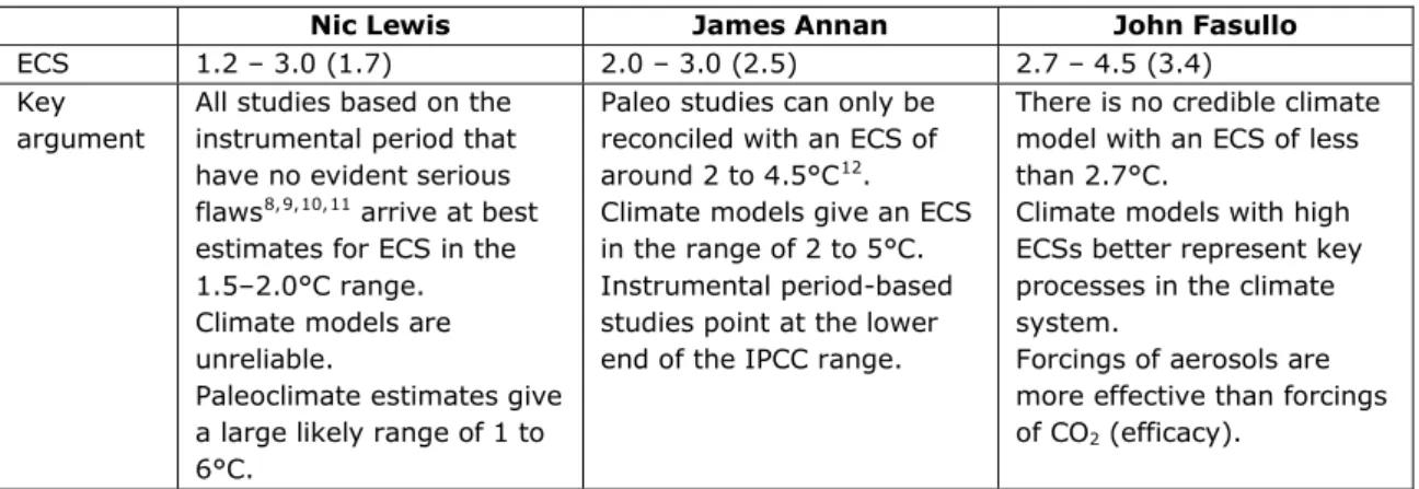
The experts’ guest blogs dealt with all questions raised in our introduction, but due to the broadness of the subject and time limitations of the participating experts, we managed to only cover the questions on ECS and not those on TCR. The Dialogue included five main topics that were discussed in more detail. The key question in this Climate Dialogue was: “What do you consider as a range and best estimate of ECS?” Table 5 summarizes the answers of the three experts and their key argument(s), which are described in more detail below.
Nic Lewis James Annan John Fasullo
ECS 1.2 – 3.0 (1.7) 2.0 – 3.0 (2.5) 2.7 – 4.5 (3.4) Key
argument
All studies based on the instrumental period that have no evident serious flaws8,9,10,11 arrive at best
estimates for ECS in the 1.5–2.0°C range. Climate models are unreliable.
Paleoclimate estimates give a large likely range of 1 to 6°C.
Paleo studies can only be reconciled with an ECS of around 2 to 4.5°C12.
Climate models give an ECS in the range of 2 to 5°C. Instrumental period-based studies point at the lower end of the IPCC range.
There is no credible climate model with an ECS of less than 2.7°C.
Climate models with high ECSs better represent key processes in the climate system.
Forcings of aerosols are more effective than forcings of CO2 (efficacy).
Table 5. Likely ranges (i.e. 66% probability) and best Estimates (between brackets) of the
ECS as estimated by the discussants.
Instrumental versus model-based approach
In his guest blog, Nic Lewis suggested that four studies based on the warming in the instrumental period6,7,8,9 are superior to the two main other methods that are available,
based on climate models and paleoclimate data. These “preferred” studies arrive at best estimates for ECS “in the 1.5–2.0°C range”. James Annan discussed both the pros and cons of the instrumental period-based estimates, calling them “more trustworthy than other approaches […]as they are more-or-less directly based on the long-term (albeit transient) response of the climate system to anthropogenic forcing” and “They point at the low end of the IPCC range due to better quality and quantity of data and better understanding of aerosol effects.”, while also mentioning that “these estimates rely on models of the climate system, which are so simple and linear (and thus certainly imperfect)”. John Fasullo agreed
with the latter remark and added that the model used in these studies captures little of the climate system’s physical complexity, since it is exclusively statistical and they only make use of “a limited subset of surface observations, questioning their relevance”. John Fasullo
indicated that “All approaches are faced with the challenges of attribution and uncertainty estimation, for which the validity of observations, the underlying model, and base assumptions are key issues. It therefore is inappropriate to place high confidence in any single approach.” Nevertheless, his best estimate and likely range (see Table 1), were mainly supported by results from studies based on climate models or so-called General Circulation Models (GCMs).
Cloud feedbacks
Doubling of CO2 in the atmosphere would give about 1.2°C of warming, assuming that
everything else remains the same. However, this warming is amplified by so-called positive feedbacks or damped by negative feedbacks. The most important positive feedbacks are an increase in atmospheric water vapour, which is a strong greenhouse gas, and the reduction in the extent of ice and snow surfaces. Additionally, in Chapter 7 of AR5, it is concluded that
8 Aldrin, M., Holden, M., Guttorp, P., Skeie, R. B., Myhre, G., & Berntsen, T. K. (2012). Bayesian estimation of
climate sensitivity based on a simple climate model fitted to observations of hemispheric temperatures and global ocean heat content. Environmetrics, 23(3), 253-271.
9Otto, A., Otto, F. E., Boucher, O., Church, J., Hegerl, G., Forster, P. M., ... & Allen, M. R. (2013). Energy
budget constraints on climate response. Nature Geoscience, 6(6), 415-416.
10Ring, M. J., Lindner, D., Cross, E. F., & Schlesinger, M. E. (2012). Causes of the global warming observed
since the 19th century. Atmospheric and Climate Sciences, 2(04), 401.
11Lewis, N. (2013). An Objective Bayesian Improved Approach for Applying Optimal Fingerprint Techniques to
Estimate Climate Sensitivity*. Journal of Climate, 26(19), 7414-7429.
12 PALAEOSENS Project Members. (2012). Making sense of palaeoclimate sensitivity. Nature, 491(7426),
changes in cloud cover “likely” represent a positive feedback although the uncertainty is large. According to John Fasullo, ECS values of below 2°C are possible only if a strong negative cloud feedback exists, which he believes is very unlikely given the conclusion of AR5. Lewis replied that he considers the conclusion of AR5 to be wrong because it is based on models which “are known to be very far from perfect.”. In the public commentary, Steven Sherwood, who was a co-author of Chapter 7 in AR5, strongly disagreed with Lewis, when he stated that the positive cloud feedback is supported by both “observations and explicit models of the relevant processes”. Andrew Dessler, a leading cloud expert, also contributing to the public commentary, likewise argued that for ECS to be as low as 1.5°C, cloud feedback needs to be strongly negative, whereas observations point to it being positive.
Lewis argued that whereas individual cloud contributions have been observed to constitute a positive feedback, there may be other, unknown contributions which still render the total cloud feedback negative.
Aerosols
An aerosol is a colloid of fine solid particles or liquid droplets, in air or another gas, such as haze or dust. On a global scale, aerosols are thought to have a net cooling effect on the climate. Aerosols thus partly compensate for the warming effect of greenhouse gases. The magnitude of their cooling effect though is highly uncertain and this has a big influence on the uncertainty in climate sensitivity. There was agreement that better constraining aerosol forcing is the key to narrowing uncertainty in ECS and TCR estimates. Lewis argued that all GCMs have larger negative forcing (i.e. cooling) for aerosols than the best estimate in AR5 (-0.9 W/m2), and as a result, the models reproduce the warming of the 20th century with a sensitivity which is (much) too high. Fasullo replied that the aerosol forcing values in models fall well within the uncertainty range of AR5, which is -0.1 to -1.9 W/m2 and therefore the
conclusion of Lewis is, according to him, unjustified. Efficacy
A related discussion was on the so-called ‘efficacy’, i.e. the hypothesis that the transient climate response (TCR and thus also ECS) to historical aerosols and ozone is substantially greater than the transient response to CO2. According to Shindell13, this is primarily caused
by more of the short-lived aerosol and ozone forcing being limited to the emission locations, which are predominantly in the continental regions of the Northern Hemisphere. Since land temperatures respond stronger to a change in forcing than ocean temperatures do, this triggers a stronger temperature response, relative to the magnitude of the forcing, than the more evenly distributed CO2 does. Annan and Fasullo indicated that estimates of ECS based
on 20th-century observations have assumed that a forcing by aerosols is equal to the same forcing by CO2, i.e. that the efficacy is 1. Kummer and Dessler14 show that the aerosol
efficacy could be as high as 1.5, which increases the instrument-based ECS estimates to a value that is similar to estimates from GCMs and paleoclimate. Lewis disagreed: “Shindell […] never refers to efficacy at all in his paper” and according to Lewis, Kummer and Dessler confuse “forcing efficacy with transient climate sensitivity” and therefore “their calculations make no physical sense.”
Paleoclimate
Changes in temperature in the distant past occurred as a result of natural forcings including e.g. changes in the Earth’s orbit and natural changes in greenhouse gas concentrations over hundreds of thousands and even millions of years. This allows the use of paleoclimatic evidence to estimate ECS. However, it should be realized that non-linearity may occur, due to the large timescale, and that then the world was very different from the way it is today with respect to, for example, ice sheet coverage, vegetation cover, the location of
13 Shindell, D. T. (2014). Inhomogeneous forcing and transient climate sensitivity.Nature Climate Change. 14 Kummer, J. R., & Dessler, A. E. (2014). The impact of forcing efficacy on the equilibrium climate
continents, mountain ridges and opening or closing of ocean passages. According to Fasullo and Annan, paleoclimatic knowledge can only be reconciled with a sensitivity in the range of 2 to 4.5°C. According to Lewis, on the other hand, the uncertainties are far too great to support this range, arguing that the likely range for paleoclimate estimates is rather 1 to 6°C.
Relevance
An additional question was raised on the relevance of the scientific debate on Climate Sensitivity to climate policy and policymakers. All of them agreed that the political debate is largely disconnected from the scientific debate on climate sensitivity, and for Lewis and Fasullo this is a problem. While Lewis argued that policymakers should listen to a wider variety of voices on climate sensitivity, including those suggesting sensitivity is low, Fasullo thinks that US policymakers who insist climate sensitivity is low, do so out of convenience, rather than on the basis of scientific evidence. For Annan, “the remaining debate concerning the precision of our [sensitivity] estimates is not, or at least rationally should not be, so directly pertinent for policy decisions. We already know with great confidence that human activity is significantly changing the global climate, and will continue to do so as long as emissions continue to be substantial”.
2.6. What will happen during a new Maunder Minimum?
The sun is a major factor in determining the Earth’s climate. However, its energy output (referred to as Total Solar Irradiance, TSI) does not seem to vary strongly over periods of decades to centuries, leading the IPCC to conclude that its influence on current global warming is very small.
According to some skeptical scientists, the sun’s influence on the current warming is much larger than assessed by IPCC and they point, for example, to correlations between cold winters in the Northern Hemisphere in the so-called Little Ice Age (LIA) and low sunspot15
activity during the Maunder Minimum in the 17th century. The LIA lasted much longer though than the Maunder Minimum and mainstream climate scientists doubt whether it was a global event.
Sunspot records, which are a well-known proxy for solar activity, suggest there has been a considerable increase in solar activity in the first half of the 20th century, leading to a Grand Solar Maximum or Modern Maximum. Some sceptics therefore claim that most of the warming before 1950 has been due to an increase in solar activity. Recently, these historical sunspot records have come under increasing scrutiny and newer reconstructions show a much ‘flatter’ sunspot history. This challenges the idea of a Modern Maximum.
Apart from the direct influence of the sun through changes in TSI, there is much attention for potential amplifying mechanisms which might explain why relatively small differences in TSI could have a larger influence on our climate. A well-known hypothesis is, for example, the effect of the sun on cosmic rays, possibly changing cloud cover and, therefore, the global amount of reflected solar radiation.16
The current solar cycle 24 (a period of approximately 11 years in which the number of sunspots goes from a minimum to a maximum) is the lowest sunspot cycle in 100 years and the third in a trend of diminishing sunspot cycles. Some solar physicists expect cycle 25 to be even smaller than cycle 24 and expect the sun to move into a new minimum, comparable with the Dalton Minimum (in the 19th century) or even the Maunder Minimum.
The current consensus among climate scientists seems to be that even when the sun enters a new Maunder Minimum this will not have a large effect on the global temperature, which will be dominated by the increase in greenhouse forcing because of its much larger magnitude.
We were very pleased that five solar scientists agreed to participate in this Climate Dialogue. Professor Mike Lockwood is Professor of Space Environment Physics with the Department of Meteorology at the University of Reading, United Kingdom. Lockwood studies variations in the sun on all timescales up to millennia and their effects on near-Earth space, the Earth's atmosphere and climate. Nicola Scafetta has been working at Duke University since 2002 and collaborates with the Active Cavity Radiometer Irradiance Monitor (ACRIM) in several projects concerning solar dynamics and solar-climate interactions. Jan-Erik Solheim is a retired professor in the field of astrophysics from the University of Tromsø, Norway. Since his retirement, he has been working as an independent scientist on some aspects of relations between the sun and the Earth and the possibility of detecting signals from planets in solar and climate variations. Professor Ilya Usoskin works at the University of Oulu (Finland). He
15 Sunspots are darks spots on the sun caused by intense magnetic activity. They have been counted since around
1610. Although these dark sunspots are cooler areas at the surface of the sun, the surrounding margins of sunspots are brighter than the average. Overall, an increase in sunspots also increases the Sun's solar brightness.
focuses his research on Solar and Solar-terrestrial physics as well as Cosmic Ray physics. José Manuel Vaquero is a lecturer in Physics of the Earth at the University of Extremadura, Spain. He is interested in the reconstruction of solar activity and Earth’s climate during the last centuries from documentary sources.
The Climate Dialogue
This Dialogue started in November 2014. Unfortunately, after the guest blogs had been published online, few of the participants had time to contribute actively to the dialogue, so in the first two months there was very little activity. Below follows a short preliminary summary that is based on the guest blogs and the first few comments.
Two of the participants (Scafetta and Solheim) clearly take a ‘sceptical’ position, which in this case means they believe the sun has contributed considerably to the 20th century warming and, therefore, the contribution of CO2 is smaller than claimed by the IPCC. Lockwood clearly
takes the ‘mainstream’ position, i.e. that the influence of the sun in terms of its energy output (Total Solar Irradiance, TSI) is very small compared to the radiative forcing of greenhouse gases. The views of the other two participants (Usoskin and Vaquero) is probably closer to Lockwood than to Scafetta and Solheim, although in their contributions they emphasise the great uncertainties and the difficulties in understanding changes in the sun back in time and its influence on our climate.
Usoskin, for example, wrote: ‘Although the present knowledge remains poor, in particular since most of the climate models consider only the direct TSI effect which is indeed quite small, I would intuitively and subjectively say that the solar influence was an important player until mid-20th century, but presently other factors play the dominant role.’ Vaquero wrote that ‘Certainly, understanding the Maunder Minimum is key for our understanding of a lot of things about the Sun and the climate of the Earth because it is a unique Grand Minimum observed using telescopes. However, our knowledge about it is quite limited.’ A key issue that needs to be discussed further is the difference between the Physikalisch-Meteorologisches Observatorium Davos (PMOD) and ACRIM time series since 1979 for the Total Solar Irradiance. These time series are based on different satellite missions that had to be stitched together. However, there is a gap of two years in the measurements in the early 1980s which has been filled differently by the PMOD and the ACRIM groups. Scafetta is involved in the ACRIM series which shows a slight upward trend between 1980 and 2000. Based on this he wrote: ‘Thus, in my opinion, the ACRIM TSI composite is closer to the truth. The sun should have experienced a secular maximum around 2000 contributing to the global warming observed from ~1970 to ~2000.’
Lockwood, and with him most mainstream climate scientists, favour the PMOD data set, which shows a small decrease between 1980 and 2000. It is as yet unclear how influential these differences between PMOD and ACRIM are for TSI reconstructions back in time, say to 1700. Such reconstructions are often based on sunspot records. But sunspot records have to be calibrated using the PMOD and/or ACRIM data set. On top of that, there is much discussion about sunspot records themselves and on their usefulness for reconstructing TSI.
3. Description of
Climate Dialogue
3.1. Approach
Climate Dialogue was set up as a moderated blog in which scientists who had published on the specific topics for discussion were invited to post blogs and comments. At least one of the invited scientists was perceived as having a sceptical point of view, i.e. rejecting (elements of) the IPCC consensus reports and arguing in favour of anthropogenic influence on global warming being lower than indicated in IPCC estimates.
The topics were selected on the basis of being controversial in climate change science and/or public debate. The objective of the blog was to organise a number of dialogues, in order to identify areas of and related reasons for agreement and disagreement within the group of participating scientists. The dialogues were technical in nature, as they zoomed in on the data, methodology and types of analyses of the topics, with frequent references to the scientific literature.
In general, the approach was the following: an introduction was written by a member of the editorial team, ending with a list of questions. The introduction was then commented and discussed by the editorial team and, in some cases, also the advisory board, until a text could be agreed upon. This then was sent to the invited scientists, asking them to write a guest blog that would contain their personal view on the topic and address the questions raised in the introduction. The moderator started the discussion by publishing the introduction and the guest blogs on ClimateDialogue.org and inviting participants to react on each other’s blog posts. The responses were moderated by a member of the editorial staff. Once a discussion had either converged or reached a standstill, it was closed by the editorial staff, although the public comment section of the blog remained open.
To round off the discussion on a particular topic, the aim was for the Climate Dialogue editor to write both an extensive and a short summary, describing the areas of agreement and disagreement among the discussants. The participants would be asked to approve this final text regarding their statements, the discussion between the experts on that topic would be closed and the editorial staff would open a new discussion on a different topic. In the first phase of the project, four discussions took place, but only one such summary had been produced. In the last phase, three more summaries were written. A summary on the sixth and final dialogue that started in November 2014 will be completed in 2015.
The general public (including other climate scientists) could comment on the blog, and these comments were shown in a separate public thread, below the invited expert thread. The public comments were approved before appearing, and if they were judged impolite, irrelevant to the main topic, or too personal, they were shown in a different thread (off-topic comments), not immediately visible, unless one clicked on them. The Climate Dialogue’s moderation policy is described on the website.