National Insitute for Public Health and the Environment
P.O. Box 1 | 3720 BA Bilthoven www.rivm.com
Emission of chemical substances from solid matrices
A method for consumer exposure assessment
RIVM Report 320104011/2010
Colophon
This investigation has been performed by order and for the account of Food and Consumer Product Safety Authority (VWA), within the framework of project 320104
‘Consumentenblootstelling’.
© RIVM 2010
Parts of this publication may be reproduced, provided acknowledgement is given to the 'National Institute for Public Health and the Environment', along with the title and year of publication.
J.E. Delmaar
Contact:
J.E. Delmaar
Centre for Substances and Integrated Risk Assessment
christiaan.delmaar@rivm.nl
Abstract
Emission of chemical substances from solid matrices A method for consumer exposure assessment
On request of the Food and Consumer Product Safety Authority RIVM has developed a method for assessing the human exposure to chemical substances emitted from solid products. This method is specifically intended for use in human exposure assessments of biocides emitted from treated articles. It can, however, be applied more broadly.
Data on model parameters, such as the coefficient of diffusion, the material air partition coefficient and the mass transfer rate, have to be available for the model to be applicable for practical exposure assessments. Data on model parameters is in many situations not available. The report presents data from literature. In cases in which representative data are not
provided, default values and methods are suggested that can be used in exposure
assessments. It should be noted that these default values will inevitably be of limited accuracy. Next to application in risk assessment for substances and biocides, the model can be used to evaluate current exposure assessment methods, such as used in REACH. It can also be used to develop alternative methods to make quick evaluations of risks, such as need in REACH. The model has been implemented in a computer program that is freely available to the general public (at www.consexpo.nl). To enhance the applicability of the method, the database on model parameters should be extended, preferably with measurement data on frequently occurring substances and materials.
Key words:
Rapport in het kort
Emissie van chemische stoffen uit vaste materialen
Een methode voor blootstellingschatting uit consumentenproducten
Het RIVM heeft in opdracht van de nieuwe Voedsel en Waren Autoriteit (nVWA) een model ontwikkeld en beschreven waarmee de blootstellingschatting voor stoffen die uit vaste
materialen vrijkomen, wordt verbeterd. Een dergelijke methode ontbreekt momenteel voor de blootstellingschatting van stoffen uit consumentenproducten. Het voorgestelde model beoogt vooral de blootstellingschatting voor biociden uit producten die met dergelijke
ongediertebestrijdingsmiddelen zijn behandeld (‘treated articles’) te verbeteren, maar kan veel algemener worden toegepast.
Om het model te kunnen gebruiken, zijn gegevens over parameters nodig, zoals de snelheid waarmee de stof zich in het materiaal verplaatst (diffusiecoëfficiënt), de vluchtigheid van de stof uit het materiaal (materiaal lucht partitiecoëfficiënt) en hoe snel het van het oppervlak van het materiaal de lucht in wordt getransporteerd (massatransfercoëfficiënt). Voor deze
parameters zijn in de literatuur waarden verzameld. Voor de gevallen waarin gegevens ontbreken, worden methoden voorgesteld om ze te schatten. Van deze methoden is de nauwkeurigheid overigens beperkt. Naast deze gegevens over parameters is een belangrijke voorwaarde voor bruikbaarheid van het model dat de beginconcentratie van de stof in de matrix bekend is.
Behalve voor toepassing in de risicobeoordeling voor stoffen en biociden kan het model ook worden gebruikt om gangbare methoden voor blootstellingschattingen, die bijvoorbeeld voor REACH worden gebruikt, te evalueren. Daarnaast kan het worden gebruikt om alternatieve methoden te ontwikkelen waarmee snelle inschattingen kunnen worden gemaakt, zoals die bijvoorbeeld nodig zijn voor REACH.
Het model is geïmplementeerd in een computerprogramma dat openbaar beschikbaar is (via www.consexpo.nl). Om de bruikbaarheid van de ontwikkelde methode te vergroten, wordt aanbevolen om de database met modelparametergegevens uit te breiden met gegevens over veelvoorkomende stoffen en producten.
Trefwoorden:
Contents
1 Introduction 13
2 Modelling the emission of substances from solid matrices 15
2.1 Model description and formulation 15
2.1.1 Model 17
2.2 Data requirements 18
2.3 Sensitivity analysis of the model 19
2.3.1 Example 1: emission of a volatile substance 21 2.3.2 Example 2: emission of a low-volatile substance 23
2.4 Summary 25
3 Data and estimation methods for the input parameters 27
3.1 Collecting data on fundamental model parameters 27
3.2 Diffusion coefficient 28
3.3 Material air partition coefficient 32
3.4 Mass transfer coefficient 37
3.5 Summary 39
4 Applying the emission model in screening assessments 41
4.1 Default values and estimation methods for model parameters 41
4.1.1 Diffusion coefficient 41
4.1.2 Material air partition coefficient 42
4.1.3 Mass transfer coefficient 42
4.1.4 Limiting situations 43
4.2 Summary 43
5 Verification of the model 45
5.1 Case 1: emission of phthalates from PVC and other materials 45
5.2 Case 2: IPBC emission from treated wood 48
5.3 Impact of sorbing surfaces: emission of DEHP from vinyl flooring 51 5.3.1 Complete model (Xu et al., 2009) parameter estimates for DEHP 52
5.4 Summary 54
6 Emission modelling tool 57
7 Discussion and recommendations 61
7.1 Emission model for substances from solid materials 61
7.2 Using the method in screening assessments 62
7.3 Recommendations 62
References 65
Appendices 67
Samenvatting
In dit rapport wordt een methode beschreven waarmee de emissie van chemische stoffen uit vaste materialen kan worden geschat. De methode is vooral bedoeld om de blootstelling van consumenten aan biociden die vrijkomen uit zogenaamde ‘treated articles’ te verbeteren. Ze kan echter ook veel algemener worden toegepast op emissies van stoffen uit diverse vaste materialen zoals vloerbedekking, behang, elektronische apparatuur et cetera.
De voorgestelde methode bestaat uit een mathematisch model dat de diffusie van de stof in het materiaal en de overdracht van materiaaloppervlak naar de binnenlucht beschrijft. Deze
methode wordt beschreven in hoofdstuk 2. Ter ondersteuning van de methode is er een literatuuronderzoek gedaan naar gegevens voor cruciale modelparameters. Dit onderzoek is samengevat in hoofdstuk 3. Aangezien gegevens van dit soort schaars zijn, zijn er ook methodes voorgesteld waarmee schattingen voor de modelparameters te maken zijn. Deze methodes geven naar verwachting redelijke orde-van-grootte bepaling van de parameters, maar zijn van beperkte nauwkeurigheid en zouden alleen ruwe karakterisering van de blootstelling moeten worden gebruikt. In hoofdstuk 4 wordt beschreven hoe de methode kan worden gebruikt in ‘screening’ van de blootstelling. De methode is in hoofdstuk 5 getest voor een aantal toepassingen waarvoor emissiegegevens bekend zijn. Deze laten zien hoe de methode kan worden toegepast, en geven inzicht in de onzekerheid in de methode. Ook is in dit hoofdstuk een nauwkeuriger, experimenteel gevalideerd model voor de emissies van matige vluchtige organische stoffen (SVOCs) vergeleken met de methode die in dit rapport wordt voorgesteld. Dit model is, in samenwerking met de Deense Environmental Protection Agency (DEPA) toegepast in een realistische blootstellingschatting. Deze modelberekeningen geven belangrijke informatie over de beperkingen in nauwkeurigheid van de in dit rapport
voorgestelde methode.
Het model dat is beschreven in hoofdstuk 2 is geïmplementeerd in een MS Windows
computerprogramma dat openbaar beschikbaar gemaakt is via www.consexpo.nl. Ten slotte wordt dit programma in hoofdstuk 6 beschreven, zowel wat betreft het gebruik van het programma als wat betreft de beperkingen in zijn toepassing.
Summary
This report discusses a method that is developed to estimate the emission of chemical substances from solid matrices. The method aims in particular to improve the exposure estimation for biocides emitted from treated articles, but can be applied much more generally to emissions of substances from various materials and products such as flooring, wall covering and electronic equipment.
The proposed method consists of a mathematical model that describes diffusion of a substance in the material and the mass transfer of the substance into bulk indoor air. The method is described in chapter 2. In support of the model a literature search on values of crucial model parameters was conducted and summarised in chapter 3. However, data on these parameters is scarce. Therefore default methods to estimate these parameters are suggested. These methods will give reasonable order of magnitude estimates, but will be of limited accuracy and should only be used for screening assessments. Chapter 4 gives a description of how the method can be applied in screening assessments of exposure. In chapter 5 the model and the methods for parameter estimation are applied in a number of cases that demonstrate the applicability of the model and also give insight in the uncertainty associated with in the use of the methods. Also, a more accurate and experimentally verified version of the model for Semi-Volatile Organic Compounds has been implemented and applied to a practical exposure
assessment for DEHP in collaboration with the Danish Environmental Protection Agency (DEPA). This model demonstrates the implications of the presence of absorption sinks in the indoor environment. The results give insight in the degree of inaccuracy of the more general model that neglects these sinks.
Finally, the model developed in chapter 2 has been implemented in a MS Windows program that is made publicly available via www.consexpo.nl. In chapter 6 the computer program is described both with respect to its use and to its limitations in application.
1
Introduction
The emission of chemical substances from consumer products may have a negative impact on the health of consumers exposed to these substances. To assess the safety of a product, the chemical exposure resulting from the use of products has to be determined. As representative measurements of exposure are mostly unavailable, prohibitively expensive or altogether impossible, the risk assessor has often to rely on the use of modelling.
Specifically, exposure to chemicals in articles (as defined in the Biocide Products Directive (BPD) Directive, REACH and EU-GHS) needs to be estimated. For such exposure assessments, little information on the release of a substance from the matrix is available. At present, standard consumer exposure modelling tools, such as the ConsExpo program (Delmaar et al., 2005) lack methods to model the release of substances from solid matrices. This hampers the applicability of these tools to important questions such as emissions of plasticisers and flame retardants from polymeric materials, and biocides from treated articles.
In current exposure assessment practice, emissions of substances from solid materials are (if at all) analysed with very crude estimation methods. Such as, for example, assuming that all the available substance will be emitted immediately or not at all, calculating the upper bound of the air concentration from the vapour pressure of the substance, et cetera. Such crude
methods are only useful to quickly screen maximum exposure levels and potential risks. In cases where such crude methods are insufficient, more realistic modelling will enable the exposure assessor to acquire a higher level of realism and accuracy, but also to make more detailed scenario evaluations (including quantitative uncertainty analysis).
In this report a model to estimate emissions of substances from solid materials is described. This model is mainly based on published work in the field of volatile organic substance (VOC) and semi-volatile organic substance (SVOC) emissions from building materials.
For a model to be applicable in regulatory exposure assessments, data on model parameters have to be known, or at least methods to make reasonable estimates for these parameters have to be available. Fundamental parameters in the proposed emission model are the diffusion coefficient of the substance in the material, the material air partition coefficient and the mass transfer coefficient. It is anticipated that for these parameters data will mostly not be available in routine regulatory assessments, as these usually require separate experiments to be
determined.
In support of the model and to enhance its applicability, a literature search was performed to collect available data and methods to estimate these fundamental model parameters. Collected data and methods can serve as a reference from which representative data may be derived in specific exposure assessments. For substances and products not represented in the database, a method is suggested to use the model in combination with default parameter values and parameter estimation methods.
The use of surrogate parameter values or estimation methods introduces a large degree of uncertainty in the modelled exposures. This generalised method is therefore only to be used as an order of magnitude estimator, and to be used in screening assessments only. If a higher degree of accuracy is needed, specific data have to be collected, or at least a quantitative analysis of the uncertainty has to be made.
The applicability of the model was tested in a number of ways:
1) By examining the changes in the results of the model to variations in the fundamental parameters, general tendencies of the model were studied. Such a sensitivity analysis provides insight in the importance of data quality and accuracy under various
conditions. Also, the relative importance of input parameters can be studied. 2) By confronting the proposed method with emission experiments under controlled
methods proposed in the generalised method, the emission of two substances from different product matrices was modelled and compared with emission experiments. These case studies, while not providing any conclusive validation, provide at least an indication of the error involved. In addition, the cases may serve as useful examples of the method.
3) For the case studies conducted in 2), the uncertainty in the method was analysed: as parameter values are not exactly known, but are subject to uncertainty, also the model outcomes will not be precise. Taking into account the imprecision in the input data, also the imprecision in the modelled exposures can be accounted for. This analysis of the uncertainty performed in 2):
4) gives insight in the overall inaccuracy of the default method;
5) serves as an example of a method that can be applied to analyse uncertainty in applications of the model in specific exposure assessments.
This report is produced for the Dutch Food and Consumer Safety Authority (VWA), which asked to develop methodology to estimate exposures of substances from articles, in particular articles treated with biocide products (treated articles). The methodology developed in this report can be used in exposure assessments of a subclass of these articles: articles of solid materials (such as wood and plastics et cetera) that have been impregnated with biocide products. For other classes of treated articles, such as textiles, other methods have to be developed. In addition to treated articles, the methods developed in this work will be applicable to other product groups. They can be used, for example, to assess exposures of SVOCs such as plasticisers from vinyl flooring, and flame retardants from electronic devices, VOCs from solid furniture and building materials et cetera.
For the purpose of this report the proposed model was build in the mathematical simulation software Mathematica. In addition, a stand-alone software tool to be used in consumer exposure assessments was built. It is available at www.consexpo.nl.
In chapter 2 the mathematical model and simplifying assumptions that have been made are described. This chapter provides the technical and scientific background of the model. An analysis of the sensitivity of the model explores the general behaviour of the model and identifies different limiting cases in which data requirements to use the model may be reduced. In chapter 3 the results of the literature search on data and methods to estimate parameters are presented. The material in this chapter can serve as a reference for the risk assessor using the model, from which data may be obtained for specific exposure assessments. On the other hand, the collected information is used to make order of magnitude inferences on the numerical values of parameters. Chapter 4 proposes default methods and data to apply the model in screening exposure assessments where information is insufficient for making accurate exposure predictions. This chapter provides guidance for a risk assessor to apply the model in exposure assessments where data is scarce. In chapter 5, the default method given in chapter 4 is tested in two cases and compared with measured emissions. The uncertainty in the method is
analysed in these two cases, which provides in indication of the degree of (in)accuracy of the method and provides examples of how to perform uncertainty analyses in regulatory exposure assessments. In section 5.3 another case study is described: the case of emission of bis(2-ethylhexyl) phthalate(DEHP) from various consumer products. This case was performed in close collaboration with the Danish Environmental Protection Agency (DEPA). In this case study the implications of including sinks such as adsorption to walls, floor and dust was investigated. Chapter 6 describes the computer program that implements the model developed in chapter 2. Chapter 7, finally, summarises and discusses the results and makes suggestions on future developments and research.
2
Modelling the emission of substances from solid matrices
Various models on the emission of substances from solid materials have been developed and used to simulate emission data. The majority of these models have been developed to estimate the emission of substances from building materials. The substance groups modelled included volatile organic substances (VOCs) such as solvents and semi-volatile organic substances (SVOCs) such as plasticisers, pesticides and flame retardants. Typically, the emission of a substance from solid materials is not only determined by volatisation of the substance and transfer from the product surface into bulk indoor air, but also by diffusional transport within the material. The latter process can usually be neglected in emission models describing the evaporation of a substance from a liquid, but may have an important effect on the emission from solid matrices.
From models as described in literature, a generalised emission model was derived. This model is described in detail in section 2.1. Section 2.2 describes the data requirements of the model. In section 2.3 a sensitivity analysis is conducted to investigate general tendencies of the model and investigate the relative importance of model parameters under different conditions.
2.1 Model description and formulation
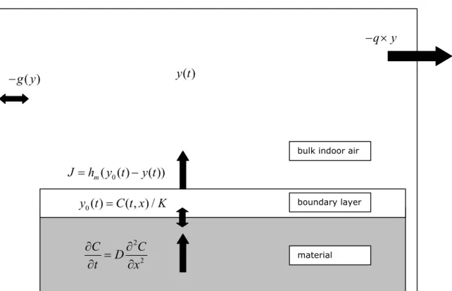
The levels of indoor air concentrations that result from the emission of substances from materials are determined by various processes (see Figure 1). On one hand there is the
emission of the substance from the material into the bulk air, on the other hand the removal of the substance from the indoor air. The first process is determined by diffusion of the substance to the surface of the material and subsequent mass transfer from surface into air. The removal of the substance from bulk indoor air is a resultant of different mechanisms such as ventilation, degradation and adsorption of the substance to indoor surfaces such as walls, furniture and dust. Adsorption is especially important for low-volatile substances such as phthalates and pesticides. When considering adsorption to indoor surfaces it should be noted that adsorbed substances may eventually desorb. This will lead to secondary emissions even after the primary source is removed.
Also, for low-volatile substances it may be that sorption to skin and clothing will give rise to dermal exposure which may be orders of magnitude higher than the exposure due to inhalation of the gas phase substance (in such cases, inhalation exposure via dust may be the most important inhalation pathway of exposure).
Figure 1. The generalised model describing the emission of (semi-)volatile substances from solid materials.
The emission of the substance is a result of diffusion in the product (characterised by the diffusion coefficient D) and mass transfer from the product surface area into bulk indoor air (characterised by the mass transfer coefficient hm). The air concentration y(t) is determined by
the emission from the material, the removal by ventilation q and additional, secondary sinks/sources g(y) such as sorption/re-emission to/from surfaces.
The model proposed in this work, is to be applied in exposure assessments for substances in articles and solid materials. Assessments of this type usually lack specificity in scenario definition and model input data. In order to keep the model applicable under general conditions, we make a number of simplifying assumptions.
1. The diffusion is usually assumed to be homogeneous and independent of the concentration of the substance in the material and can thus be described with a constant diffusion coefficient D.
2. Only the removal of material from the bulk (room) air by ventilation is considered. Other sinks, such as the adsorption to dust, indoor surfaces and degradation of the substance are discarded. This assumption will possibly lead to an overestimation of the air concentrations in the early stages of emission, but may underestimate the air concentrations due to secondary (re-)emissions, that may still occur when the emitting material has been removed or is depleted. This assumption is likely to be inaccurate for poorly evaporating (low vapour pressure) substances such as SVOCs. In section 5.3 the implications of neglecting sinks are studied in a specific example.
3. Emission of the substance is only from the top surface of the material. The other surfaces (i.e. the sides and bottom of the material) are supposed to be covered or to be so small as not to give a significant contribution to the emission.
0
( )
( , ) /
y t
C t x K
2 2C
C
D
t
x
0( ( )
( ))
mJ
h y t
y t
material boundary layer bulk indoor airq y
( )
g y
It should be noted that these assumptions will limit the accuracy of the modelled emissions. To what extent the accuracy is hampered will depend on the specific application (e.g. type of substance, product material, time scale of the assessment, indoor environment). On the whole, the model should not be expected to accurately estimate realistic concentration levels under all circumstances, but rather serve as an estimation tool to screen order of magnitude exposure levels.
2.1.1 Model
In the model the material is modelled as a slab of thickness L. With the assumptions described above, the concentration C in the material is determined by a one-dimensional diffusion equation: (1) 2 2
C
C
D
t
x
Where t is the time, x is the depth in the material and D the diffusion coefficient. In our model formulation we further assume that emission takes place only at the surface of the material. Depending on the material the diffusion can be either the solid state diffusion or the gas phase diffusion. The latter is important for porous materials.
For materials with porosity ε, and assuming that gas phase diffusion dominates over solid state diffusion, equation 1) transforms to
(2) 2 gas ad gas gas 2
C
C
C
(1
)
D
t
t
x
Cad is the adsorbed concentration, which, under isothermal conditions is related to the gas
phase concentration Cgas by Cad = KsCgas (with Ks the material surface air partition coefficient).
Hence it follows that,
(3)
2 2
gas gas gas * gas
2 2 s
C
D
C
C
D
t
(1
)K
x
x
Note that the mathematical form of this equation is completely identical to equation 1). In other words, the existence of a gas phase transport in addition to the solid state transport can be included by introducing a modified, ‘effective’ diffusion coefficient D*.
To evaluate the concentration in the material, equation 1) or 3) should be solved with
appropriate boundary conditions. In most practical applications the initial concentration C0 can
be assumed to be homogeneous. Its numerical value has to be known and specified in the model.
From assumption 3) above, it follows that at the bottom side (or at the sides) of the material there is no flux of substance out or into the material:
(4a) x 0
C
0
x
(4b) x L
C
J
D
x
This flux of substance from the material surface equals the flux through the stagnant boundary layer in the air above the surface:
(4) m 0 x L
C
D
h (y (t) y(t))
x
Under isothermal conditions, the air concentration
y
0directly above the surface is assumed to be proportional to the material concentration C(x=d):(5) 0
x L
y
C
K
With K as the material air partition coefficient of the substance.
The mass transfer coefficient hm describes the transport velocity of the substance from the
material surface to the bulk indoor air y. The bulk air concentration is assumed to be homogeneous (well-mixed). It is determined by the emission from the material and the removal by ventilation:
(6)
y
Sh
m(y
0y) qy
t
V
With q the ventilation fold of the room, S the surface area of the material, and V the volume of the room.
The simplified diffusion model 1-7 with the given boundary conditions can either be solved analytically (as an infinite sum) or numerically (for example by finite difference methods).
2.2 Data requirements
In order to apply the emission model in practical exposure assessments, the following data are needed as input (units are specified in SI, but can be provided in any other consistent system of units):
Specifics of the material:
S: surface area of the material [m2]
L: thickness of the material [m] Co: initial concentration in the material [kg/m3]
Data on the indoor environment:
V: volume of the room [m3]
q: ventilation fold of the room [s-1]
D: diffusion coefficient [m2/s]
K: material air partition coefficient [-] hm: mass transfer coefficient [m/s]
In a typical case, data on material and the indoor environment will be known or chosen as part of a scenario when the model is used in an exposure assessment. The physical chemical data, on the other hand will mostly not be available.
To enhance the usability of the model, a literature search was performed to collect data on these physical chemical parameters, and estimation methods for these parameters. The resulting database and estimation methods can be used as a reference from which
representative data may be selected in regulatory exposure assessments. The results of this literature survey are presented in chapter 3.
2.3 Sensitivity analysis of the model
Lack of accurate data on the physical chemical input data will be an issue in many situations in which the emission of substances from solid matrices has to be estimated. In this section, an analysis of the sensitivity of the model is made over the ranges of the parameter values that are expected to occur in practical applications. This analysis will identify general tendencies of the model and will identify situations in which the model is insensitive to variations in one or more of the model parameters. In these situations, the data requirements are effectively reduced.
The out flux of substance material is given by:
(7) x L
C
D
x
In steady state this out flux has to equal the transport flux over the boundary layer:
(8) m x L
C
C(L)
D
h (
y)
x
K
If we approximate this by:
(9)
D
C(L) C(0)
h (
mC(L)
y)
L
K
and solve for the unknown material concentration at the surface C(L), we find:
(10) m
DK
Ky
C(0)
Lhm
C(L)
DK
1
Lh
From this it is seen that for D/L >> hm/K: m
DK
1
Lh
and mDK
C(0)
Ky
Lh
(asKy C(0)
). From this it follows that:C(L) C(0)
In other words, the concentration in the material is homogeneous:
C(x, t) C(t)
, independent of x.Then the emission into bulk indoor air (equation (6)) is given by:
(11)
dy
h S
m(
C(t)
y) qy
dt
V
K
And the change in concentration C in the material is reduced to:
(12)
dC
h
m(
C(t)
y)
dt
L
K
Note that the diffusion coefficient D has been eliminated from these equations. The system is independent of the exact value of D (as long as D/L >> hm/K). This situation is referred to as
being mass transfer limited.
Conversely, if D/L << hm/K:
C(L) Ky
And from equations (4) and (6): (13) x L
dy
S
C
D
qy
dt
V
x
And the emission is independent of the exact value of hm/K. The emission is diffusion limited.
The existence of two limiting cases, mass transfer and diffusion limited emission, has important implications for practical exposure evaluations: in the first case (diffusion limitation) it is not important to know the exact value of hm/K. In the other case (mass transfer limitation) it is not
important to know the diffusion coefficient D with high accuracy. In these situations the efforts in data collection may be reduced significantly.
However, it is important to keep in mind that the discussion above is only approximate. For example, in (9), the approximation
D
C
D
C(L) C(0)
x
L
is made. This can only be done if the diffusion lengthL
dif
2 Dt
is of order L. For short times, this approximation may be inappropriate and the limiting situation (mass transfer or diffusion limitation) will only be in effect after the initial stages of emission.2.3.1 Example 1: emission of a volatile substance
As an example, consider the emission of a volatile substance (vapour pressure > 10 Pa) from a (fictitious) product made of a material similar to vinyl. The product has a layer thickness of about 0.01 m. hm depends on product shape and indoor conditions (airflow over the surface).
As will be shown in chapter 3, hm typically lies in a range of ~ 0.0005 – 0.005 m/s. Diffusion
coefficients of substances in vinyl flooring are in a range of 10-10 – 10-13 m2/s (see chapter 3),
for this example a range of 10-10 – 10-12 m2/s was assumed.
In the example, the following parameter values are used:
room volume V 20 m3
ventilation rate q 1 hr-1
product surface area S 0.5 m2
product thickness L 0.01 m
product concentration Co 1 kg/m3
exposure duration 50 hr
diffusion coefficient D 10-10 – 10-12 m/s2
Typically, material air partition coefficients for volatile substances are between 1 – 1000 (discussed in chapter 3).
For this case, D/L was varied between 10-8 – 10-10 m/s, and h
m/K was varied between 5x10⁻³ –
5x10⁻⁷ m/s.
The air concentration resulting from the emission is simulated with the model for different values of D/L and hm/K. For different simulations hm/K was kept fixed at:
1) the lower extreme of its estimated range (hm/K = 5x10⁻³);
2) the higher extreme of its estimated range (hm/K = 5x10⁻⁷).
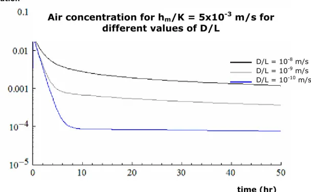
For both cases 1) and 2) D/L was varied in discrete steps over its entire range. The results are plotted in Figure 2 for case 1) and Figure 3 for case 2).
In these simulations it can be observed that:
- The estimated air concentrations depend strongly on the value of D/L: concentration levels vary approximately linearly with the value of D/L.
- The estimated air concentrations are insensitive to changes in the value of hm/K.
That is, within the ranges of parameter values for this case the model is diffusion limited, as is expected based on the formal considerations above (equation (13)).
Figure 2. Log-linear plot of the variation of the air concentration with D/L for a fixed value of hm/K of 5x10⁻⁷ m/s over the entire simulation duration (50 hrs).
Figure 3. Log-linear plot of the variation of the air concentration with D/L for a value of hm/K of
5x10⁻³ m/s over the entire simulation duration (50 hrs).
time (hr)
concentration (g/m3) D/L = 10-8 m/s D/L = 10-9 m/s D/L = 10-10 m/sAir concentration for h
m/K = 5x10
-7m/s for
different values of D/L
concentration (g/m3)time (hr)
D/L = 10-8 m/s D/L = 10-9 m/s D/L = 10-10 m/sAir concentration for h
m/K = 5x10
-3m/s for
2.3.2 Example 2: emission of a low-volatile substance
As a second example, consider the emission of a semi-volatile substance (vapour pressure < 10 Pa) from a (fictitious) solid product. In this case the material air partition coefficient is typically larger than about 100,000 (see chapter 3, Table 3). Taking, as an example, a range of [1.0 x 10⁶ – 1.0 x 10⁸] for the material air partition coefficient, and a typical value of 1 x 10 -4 m/s for the mass transfer rate, we find a range of [1 x 10⁻¹⁰ – 1 x 10-12] m/s for h
m/K.
Similar to the procedure followed in example 1, model simulations were conducted for the ranges of both D/L and hm/K. In this case, D/L was kept at a fixed value during a single
simulation and hm/K was varied in discrete steps over its entire range. Two different
simulations were performed, for D/L = 10-6 and 10-8 m/s respectively. The emission duration
was chosen as 200 hours. All the other model input parameters were kept at fixed values (the same as in example 1).
In summary, the following parameter values were used in the simulation:
room volume V 20 m3
ventilation rate q 1 hr-1
product surface area S 0.5 m2
product thickness L 0.01 m
product concentration Co 1 kg/m3
exposure duration 200 hr
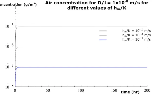
From the results of the simulations, shown in Figure 4a and Figure 4b, a clear dependence on hm/K is observed. The air concentration levels vary roughly linearly with hm/K. On the other
hand, the concentration levels are independent of the exact value of D/L (within its range), as can be observed by comparing Figures 4a and 4b. The emission is mass transfer limited, as expected for these values of hm/K and D/L.
0
50
100
150
200
10
8
10
7
10
6
10
5
Figure 4a. Log-linear plot of the variation of the air concentration with hm/K for a value of D/L
of 1x10⁻⁶ m/s over the entire simulation duration.
0
50
100
150
200
10
8
10
7
10
6
10
5
Figure 4b. Log-linear plot of the variation of the air concentration with hm/K for a value of D/L
of 1x10⁻⁸ m/s over the entire simulation duration.
hm/K = 10-10 m/s hm/K = 10-11 m/s hm/K = 10-12 m/s concentration (g/m3)
time (hr)
Air concentration for D/L= 1x10
-6m/s for
different values of h
m/K
concentration (g/m3)time (hr)
hm/K = 10-10 m/s hm/K = 10-11 m/s hm/K = 10-12 m/sAir concentration for D/L= 1x10
-8m/s for
different values of h
m/K
2.4 Summary
This chapter describes the scientific formulation and background of a model that can be used to more realistically simulate the emission of substances from solid materials. The model takes into account the diffusion of the substance in the material, the transfer of the substance from the material surface into indoor air, and the removal of the substance from indoor air by ventilation. The model assumes that:
- the emission takes place indoor;
- the concentration of the substance in the material and the material itself are homogeneous;
- the emission is from one large surface area (the top side of a plate, thin slab of material or a thin layer of product) and not from the sides of the product. Emission of other product shapes are not adequately described by the model formulated above. However, the model can easily be adjusted to include other (simple) product geometries.
Additional removal processes, such as the addition of the substance to surfaces and dust and degradation of the substance are not included. These simplifications will limit the accuracy of the modelling results, especially in the case of the low-volatile substances (substances with vapour pressure of ~10 Pa and lower). The effect of neglecting additional sinks will be that during emission from the material, air concentrations will be overestimated, however air concentrations after depletion or removal of the material may be underestimated by the model. In section 5.3 the effects of neglecting sinks will be studied in a specific example.
A sensitivity analysis of the model demonstrates the existence of two limiting cases,
determined by the quotient of D/L and hm/K. In the case of mass transfer limitation (D/L >>
hm/K) the emission is mostly determined by the material air partition coefficient K and the mass
transfer rate hm. The exact value for D is not critical. This, in effect, reduces the need to collect
precise numerical data on D. In the case of diffusion limitation (D/L << hm/K), emission is
mostly determined by D, and accurate determination of K and hm are less critical under most
conditions. This information is useful to simplify exposure assessments in many practical applications. As a rule of thumb, emissions of SVOC (and other low vapour pressure substances) from solid materials will be mass transfer limited and the emission of volatile substances will be diffusion limited. However, in any exposure assessment, it is recommended to verify the value of the quotient of D/L and hm/K.
3
Data and estimation methods for the input parameters
3.1 Collecting data on fundamental model parameters
In order to be able to use the model described in chapter 2, numerical values of a number of fundamental model parameters has to be known. These are:
the diffusion coefficient D of the substance in the material; the mass transfer coefficient hm;
the partition coefficient K of the substance between the material of the product and air. Data on these parameters are scarce. The data that are available are mostly derived from research on VOC emissions from building materials. More recently, limited data on emissions of SVOCs from building materials have been published. Limited data on substances in polymeric matrices are also reported in literature.
In this section an overview is given of data and methods for parameter estimation published in literature. These data and methods may serve as a reference database to be used in consumer exposure assessments. It should be noted however, that the database is far from complete. Data and methods provided here, may serve as surrogate values in cases where adequate data is missing, but will not be a substitute for specific data on the substance and product.
Extending the database with data on important substance/material combinations would greatly increase the applicability of the model.
Experimental data on model parameters are typically obtained in one of two ways: 1) from publications on a completely parameterised version of the model (or a similar
version thereof), describing an experimental emission situation; 2) from direct measurements of the parameter.
The latter option often applies to either simultaneous measurement of the diffusion coefficient D and the partition coefficient K, or separate measurements of partition coefficients.
Data from publications that were found in literature are summarised in Tables 1-4, on diffusion coefficient and partition coefficient respectively.
Apart from reporting numerical values for model parameters, some authors also provide methods to estimate values for these parameters. Mostly, these methods are based on experimental observations of correlations between the parameter value and properties of the substance and the matrix, such as molecular weight or vapour pressure. Usually, these methods are derived in a specific domain, and have only been tested for a limited set of substances and materials.
Numerical values for the parameters and estimation methods are discussed in the next sections. Section 3.2 summarises data on diffusion coefficients, section 3.3 on the material air partition coefficient, and section 3.4 is on methods to estimate the mass transfer rate.
3.2 Diffusion coefficient
Diffusion coefficients of substances in solid materials will depend on many aspects, such as the size and shape of the molecules of the diffusing substance, on the molecular properties of the matrix and on the porosity of the product material.
Welty et al. (2007) report that, as a rough indication, diffusion coefficients of substances in (non-porous) materials typically lie in the range of 10-12 – 10-14 m2/s.
Table 1 summarises experimental data on diffusion coefficients found in literature. Most of the data are obtained in the fields of VOC emissions from building materials and the migration of substances from polymeric matrices. The reported diffusion coefficients were determined at about room temperature (between 20-23 oC).
Table 1. Summary of diffusion coefficients published in literature.
Substance Matrix/product D [m2/s]
(x 1011) Molecular weight1
(g/mol)
Study
toluene carpet backing 4.31 92.14 Bodalal et al., 2000
nonane carpet backing 2.83 128.26
vinyl floor tile 1.48
decane carpet backing 0.54 142.29
plywood 1.28
vinyl floor tile 0.21
undecane carpet backing 0.28 156.31
vinyl floor tile 0.09
cyclohexane plywood 15.5 84
ethylbenzene plywood 4.04 116.25
vinyl floor tile 1.6
water vinyl flooring 0.36 18 Cox et al., 2001
n-butanol “ 0.067 74 toluene “ 0.069 92 phenol “ 0.012 94 n-decane “ 0.045 142 n-dodecane “ 0.034 170 n-tetradecane “ 0.012 198 n-pentadecane “ 0.0067 212
hexanal oriented strand board 0.18 100.16 Yuan et al., 2007
styrene polysterene foam 0.62 104.15
TVOC particle board 7.7 Yang, 2001
Hexanal “ 7.7 100.16
α-pinene “ 12 136.24
2004 concrete 4.33 gypsum board 1270 carpet 1030 wallpaper 0.28 n-octane brick 140 114.23 concrete 1.69 gypsum board 1200 carpet 3560 wallpaper 0.42
styrene carpet 1 (nylon fibre, polypropylene backing, styrene-butadiene rubber latex adhesive ) 0.4 104.15 Little et al., 1994 carpet 4 (polypropylene and nylon fibres, polypropylene backing, styrene-butadiene rubber latex adhesive) 0.31 4-ethenylcyclohex ane carpet 1 0.52 110.2 carpet 4 0.21
methane low density
polyethylene 1.9 16 Piringer, 2008 methane “ 3.0 16 ethane “ 0.48 30 ehtane “ 0.54 30 methanol “ 0.48 32 propane “ 0.52 44 n-pentane “ 0.08 72 benzene “ 0.11 78 benzene “ 0.04 78 n-hexane “ 0.11 86 n-hexane “ 0.084 86 phenole “ 0.045 94 heptanol “ 0.053 116 2,3-benzopyrole “ 0.055 117 2-phenyl-ethyl-alcohol “ 0.043 122 3-octene-2-one “ 0.073 126 n-octanal “ 0.023 128 4-isopropyl-toluene “ 0.054 134 limonene “ 0.043 136 3-phenyl-1-propanol “ 0.028 136 n-Nonanal “ 0.018 142
7-methyl-chinoline “ 0.043 143 2,3,5,6 tetramethyl-phenol “ 0.016 150 dimethyl-benzyl-carbinol “ 0.0075 150 3,7-dimethyl-6-octene-1-al “ 0.01 154 n-decanal “ 0.014 156 3,7-dimethyl-octene-3-ol “ 0.013 158 diphenyl-oxide “ 0.037 170 n-dodecane “ 0.026 170 dimethyl-phthalate “ 0.019 194 n-tetradecane “ 0.019 198 tetradecanol “ 0.0082 214 2,6-di-tert- butyl-4-methyl-phenol “ 0.0048 220 cedrylacetate “ 0.0041 264 eicosane “ 0.0063 282 docosane “ 0.0035 310 timuvin 326 “ 0.002 315.8 2-hydroxy-4-ethandiol methyl-thioacetic acid ester “ 0.0009 346 methyl-tricosanate “ 0.0015 368 methyl-octacosanate “ 0.0003 438 didodecyl-3-3- thio-dipropionate “ 0.0002 514 3-(3,5—di-tert-butyl-4-hydroxy phenyl)-propionate “ 0.00011 531
1 If the molecular weight was not given in the cited reference, it was taken from the SRC Inc.
Diffusion coefficient D vs molecular weight 1.E-15 1.E-13 1.E-11 1.E-09 1.E-07 0 100 200 300 400 500 600
molecular weight (g/mol)
D (
m
2/
s)
Figure 5. Plot of the diffusion coefficients D reported in Table 1 versus the molecular weight of the substance for all different matrices.
It is observed that the parameter values for the compound/material combinations reported here span a range from about 10-10 - 10-13 m2/s. Diffusion in porous materials will consist of
both gas and material phase diffusion and will usually be faster (as is seen, for example for ethyl acetate and n-octane in brick). Not many data on the diffusion in porous materials have been found. This lack of data constitutes an important data gap at present.
The diffusion coefficient is expected to correlate with both the molecular weight of the diffusing substance and the molecular weight of the matrix. The latter is not known for most matrices and products reported in Table 1. In Figure 5 the reported diffusion coefficients have been plot versus the molecular weight of the diffusing substance. A tendency of the diffusion coefficient to decrease with increasing molecular weight is observed. Given an extensive set of good quality data, it might be possible to make quantitative inferences on the diffusion coefficient based on only the molecular weight of the diffusing substance. However, the present database is too small to be used for this purpose.
Several empirical relations have been derived to estimate the diffusion coefficient for groups of substances and materials (summarised in Guo, 2002b).
The most general is the relation proposed in both (Bodalal et al., 2000) and (Cox et al., 2001):
(14) n w
A
D
m
in which D is the diffusion coefficient (m2/s), m
w is the molecular weight (g/mol), and A and n
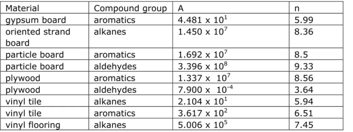
Values for A and n are given for different materials and compound groups (taken from Guo, 2002b):
Table 2. Parameters for the empirical model proposed by Guo, equation (14).
From the data and estimation methods presented here representative values can be derived for similar product/material combinations. The question remains to what extent the materials and substances reported here are representative for other substances and materials. Also, porous materials are underrepresented in the database.
To enhance the models applicability, the database should be expanded to include reference values for materials and substances frequently encountered in regulatory assessments, such as wood, plastic et cetera.
3.3 Material air partition coefficient
Table 3 summarises experimental data on material air partition coefficients found in literature. Most of the data is obtained in the field of VOC emissions from building materials. In this document the partition coefficient is defined as the quotient of the (equilibrium) material concentration Cmat and the air concentration Cair. Another definition of the material air partition
coefficient is defined as the ratio of the (equilibrium) material surface concentration and the air concentration. In this report we refer to this partition coefficient as the surface material air partition coefficient. This partition coefficient describes the adsorption to a surface rather than partition into a material. Whereas the former definition of the partition coefficient is a
dimensionless number, the latter has dimensions of [length]. In this report we are mainly interested in the first, dimensionless partition coefficient, however, also adsorption partition coefficients are reported in a separate table. These surface partition coefficients will be useful when sorption to surfaces is included in the model. The surface air partition coefficients are reported in Table 4.
Material Compound group A n
gypsum board aromatics 4.481 x 101 5.99
oriented strand board
alkanes 1.450 x 10⁷ 8.36
particle board aromatics 1.692 x 10⁷ 8.5
particle board aldehydes 3.396 x 10⁸ 9.33
plywood aromatics 1.337 x 10⁷ 8.56
plywood aldehydes 7.900 x 10⁻⁴ 3.64
vinyl tile alkanes 2.104 x 101 5.94
vinyl tile aromatics 3.617 x 10² 6.51
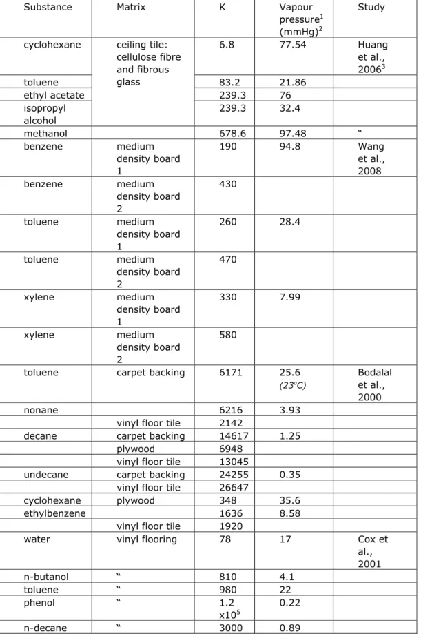
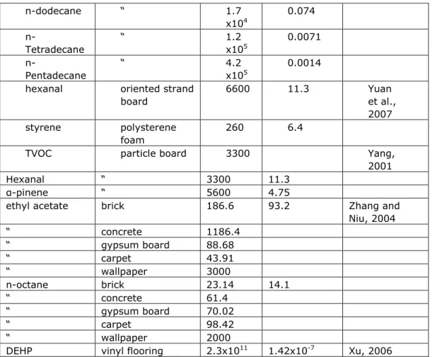
Table 3. Summary of material air partition coefficients for various material/substance combinations published in literature.
Substance Matrix K Vapour
pressure1 (mmHg)2 Study cyclohexane 6.8 77.54 Huang et al., 20063 toluene 83.2 21.86 ethyl acetate 239.3 76 isopropyl alcohol ceiling tile: cellulose fibre and fibrous glass 239.3 32.4 methanol 678.6 97.48 “ benzene medium density board 1 190 94.8 Wang et al., 2008 benzene medium density board 2 430 toluene medium density board 1 260 28.4 toluene medium density board 2 470 xylene medium density board 1 330 7.99 xylene medium density board 2 580
toluene carpet backing 6171 25.6
(23oC)
Bodalal et al., 2000
nonane 6216 3.93
vinyl floor tile 2142
decane carpet backing 14617 1.25
plywood 6948
vinyl floor tile 13045
undecane carpet backing 24255 0.35
vinyl floor tile 26647
cyclohexane plywood 348 35.6
ethylbenzene 1636 8.58
vinyl floor tile 1920
water vinyl flooring 78 17 Cox et
al., 2001 n-butanol “ 810 4.1 toluene “ 980 22 phenol “ 1.2 x10⁵ 0.22 n-decane “ 3000 0.89
n-dodecane “ 1.7 x10⁴ 0.074 n-Tetradecane “ 1.2 x10⁵ 0.0071 n-Pentadecane “ 4.2 x10⁵ 0.0014
hexanal oriented strand
board 6600 11.3 Yuan et al., 2007 styrene polysterene foam 260 6.4
TVOC particle board 3300 Yang,
2001
Hexanal “ 3300 11.3
α-pinene “ 5600 4.75
ethyl acetate brick 186.6 93.2 Zhang and
Niu, 2004 “ concrete 1186.4 “ gypsum board 88.68 “ carpet 43.91 “ wallpaper 3000 n-octane brick 23.14 14.1 “ concrete 61.4 “ gypsum board 70.02 “ carpet 98.42 “ wallpaper 2000
DEHP vinyl flooring 2.3x10¹¹ 1.42x10⁻⁷ Xu, 2006
1 The reported vapour pressures are taken from the publication. If the study did not report a value for the vapour pressure, it was obtained from the SRC PhysProp database (http://www.srcinc.com/). Reported values are determined at about room temperature (20-23 oC).
2 Units used in the model formulations in this document are in SI. To convert the vapour pressure to SI units (Pa), multiply by
133.32
3 Calculated from [mg/kg solid]/[mg/ kg air] using ρsolid = 261 kg/m3 and ρair = 1.2 kg/m3.
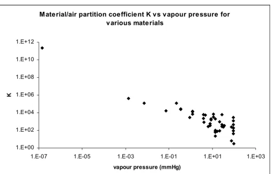
The material air partition coefficient is expected to anti-correlate with the vapour pressure. Figure 6 plots K versus the vapour pressure on a double log scale for all materials and substances reported in Table 3. A negative correlation is observed. However, the database seems too small to make any general quantitative inferences. Especially, low-volatile materials are underrepresented.
Figure 6. Material air partition coefficients from Table 3 plotted versus the vapour pressure of the substance.
No distinction is made between materials and the weight fraction of the substance in the material.
Material/air partition coefficient K vs vapour pressure for various materials 1.E+00 1.E+02 1.E+04 1.E+06 1.E+08 1.E+10 1.E+12
1.E-07 1.E-05 1.E-03 1.E-01 1.E+01 1.E+03
vapour pressure (mmHg)
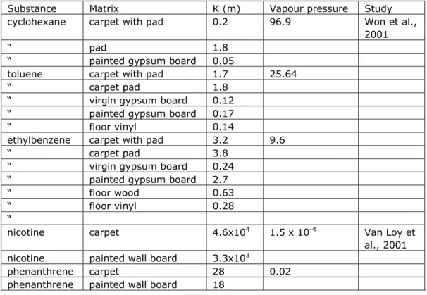
Table 4. Summary of surface air partition coefficients for various material/substance combinations published in literature.
In addition to numerical values published for partition coefficients, a number of authors have developed empirical correlations that link material air concentrations to the vapour pressure of the compound for specific materials and substance groups (Zhao, 1999; Bodalal et al., 2000). Based on these, Guo (2002b) suggests a ‘universal’ relation:
(15)
ln K 8.76 0.785ln P
In this equation, the vapour pressure P is in mmHg.
This relation was developed using a set of 56 material/compound (exclusively building materials and VOCs) combinations and estimates the partition coefficients for the training set within 2 orders of magnitude. It should be kept in mind however, that this relation can most likely not be used for non-VOC substances and materials that are very different from the ones used in the training set.
Weschler and Nazaroff (2008) studied the fate of semi-volatile substances (SVOCs) such as plasticisers, pesticides and flame retardants in indoor environments. For the emissions from material into air they suggest, as an order of magnitude estimation method, to use Raoult’s law for estimating a partial vapour pressure and its corresponding saturated air concentration. Raoult’s law is formulated as:
(16) part vap sub vap
sub rest
n
P
xP
P
n
n
Substance Matrix K (m) Vapour pressure Study cyclohexane carpet with pad 0.2 96.9 Won et al.,
2001
“ pad 1.8
“ painted gypsum board 0.05
toluene carpet with pad 1.7 25.64
“ carpet pad 1.8
“ virgin gypsum board 0.12 “ painted gypsum board 0.17
“ floor vinyl 0.14
ethylbenzene carpet with pad 3.2 9.6
“ carpet pad 3.8
“ virgin gypsum board 0.24 “ painted gypsum board 2.7
“ floor wood 0.63
“ floor vinyl 0.28
“
nicotine carpet 4.6x10⁴ 1.5 x 10⁻⁴ Van Loy et
al., 2001 nicotine painted wall board 3.3x10³
phenanthrene carpet 28 0.02
where x is the molar fraction of the SVOC in the product matrix, and nsub and nrest are particle
number concentrations of the substance and the rest of the compounds in the matrix respectively.
Assuming that Raoult’s law is a reasonable estimate of the driving pressure, we can derive for the air concentration at the surface Cair:
(17) air sub part sub sub vap sub rest
m
m
n
C
P
P
RT
RT n
n
where use has been made of the ideal gas law.
R is the universal gas constant, T the absolute temperature, msub the molecular weight of the
evaporating substance. Now, making use of i i
i
w
n
m
for the particle number concentrationn
iof component i in the material (
is the density of the product,m
i andw
i are is the mol weight and the weight fraction of component i in the matrix respectively):(18) sub sub sub sub i i sub rest sub sub i i i sub i
w
n
m
1
C
w
w
w
n
n
w
m
m
m
m
If this is substituted this in (16), it is observed that this relation is not linear in
w
sub (and thus Cmat), and the resulting expression can not be interpreted as linear partitioning. But insituations that
w
sub in the denominator of (18) may be neglected, we may define a (linear) partition coefficient K as:(19) sub sub i i
i i
air vap sub i vap i
w
w
C
RT
RT
K
[w
m
]
C
P m
m
P
m
i sub i subw
w
(
)
m
m
In this, use was made of
C w
sub
.If experimental values for the vapour pressure are not available, the authors recommend the use of the ‘SPARC’ tool (http://ibmlc2.chem.uga.edu/sparc/), that was found to produce satisfactory results for a large number of substances, providing estimates usually within one order of magnitude deviation from measured values.
3.4 Mass transfer coefficient
Under typical indoor conditions, emission of a substance from a material into air is hampered by a layer of stagnant air (the so-called boundary layer) above the emitting surface. The mass transfer coefficient describes the diffusional transport over this layer (see, for example, Welty et al., 2007). The shape of the boundary layer (and thus the mass transfer coefficient) depends on the geometry of the emitting material, surface roughness of the material, and the airflow over the surface. Theoretical descriptions of various surface configurations have been developed. The method most commonly used in engineering applications is the one as
described for example in (Kiil, 2006), which uses the theoretical correlation between Sherman, Reynolds and Schmidt numbers (Sh, Re, Sc) for a flat plate and laminar flow conditions over the material surface. From this relation it follows that:
(20)
h
m
0.664 D
air
Re
1/ 2
Sc / L
1/3 sysReynolds (Re) and Schmidt (Sc) numbers are given by:
sys
v
Re L
airSc
D
from which: (21) m air2 / 3 1/ 6 1/ 2 sysv
h
0.664D
(
)
L
In these equations, Lsys is a typical length of the system,
v
the velocity of the air over thesurface,
the kinematic viscosity of air (1.5x10⁻⁵ m2/s at 25 oC), airD
the diffusion coefficient of the substance in air.Sparks et al. (1996) suggest that the theoretical correlation (20) for a flat plate is not appropriate as indoor air movement is not uni-directional. They determined the experimental correlation between Nusselt, Reynolds and Schmidt numbers (Nu, Re and Sc) for a cylindrical cup filled with pure p-dichlorobenzene. Schmidt, Reynolds and Nusselt numbers were
determined for a range of representative indoor air velocities over the surface of 0.05 – > 0.6 m/s.
The authors suggest the following experimental correlation to predict the mass transfer coefficient:
0.67
m air sys
h
0.33 D
Re
/ L
In their work, it appears that ‘Nusselt number’ (which refers to convective heat transport) is used synonymously with Sherman number.
It should be noted that also in this case, in which the mass transfer correlation was determined by experiment, the adequacy of the proposed method depends on to what extend the
experimental set up (emission from a cylindrical cup) is representative of the realistic emission conditions.
Below, in Figure 7, the predicted mass transfer coefficients for the two methods are plotted as a function of the air velocity over the surface. For the diffusion coefficient in air a typical value of 1.0 x 10⁻⁵ m2/s was used. The emitting source was supposed to have a characteristic
dimension of 1 m.
In this case the results of both methods differ by up to a factor of 3. The prediction by the flat plate method gives the higher estimates.
Comparison of Sparks and flat plate methods for estimating
the mass transfer coefficient
0 0.0005 0.001 0.0015 0.002 0.0025 0.003 0.0035 0.004 0.0045 0 0.2 0.4 0.6 0.8
air velocity over surface (m/s)
m ass tr an sfe r co ef fi ci en t (m /s ) hm (m/s) flat plate hm (m/s) sparks
Figure 7. Example of mass transfer coefficients calculated by the flat plate correlation method and Sparks’ method (Sparks et al., 1996) respectively.
For a typical air diffusivity Dair of 1.0 x 10⁻⁵ m2/s and surface air velocities between 0.05 and
0.6 m/s. The flat plate method generally gives higher estimates of the mass transfer, leading to higher predictions of the emission rate.
3.5 Summary
Data on critical parameters D, K and hm of the model are scarce. The available data is mostly
for VOC and SVOC emissions from building materials. Also a reasonable amount of data on diffusion coefficients in polyethylene was found. The collected data may serve as a reference for exposure assessors. However, data for many important substances and products is not available. Ranges of values for the diffusion coefficient were derived from the collected data, for the mass transfer coefficient, reasonably accurate estimation models exist, for the material air partition coefficient K data is especially scarce. A very crude estimation method was suggested by Weschler and Nazaroff (2008) which may be useful as a first approximation. However, the inaccuracy of this method is unknown, but likely to be very high. The estimation methods and parameter value ranges are only approximate and can not be a substitute for case-specific data. Collection of more data on these fundamental model parameters (especially the partition coefficient K) will greatly enhance the usability of the model and the overall quality of the exposure assessment.
4
Applying the emission model in screening assessments
The model proposed in chapter 2 to simulate emissions of substances from a solid product matrix includes a detailed description of the transport of a substance within the material to the surface, and subsequent transport from the surface into bulk indoor air. As such, the model is a realistic representation of the actual emission process. In the case where adequate input values for the model parameters are given (most notably, the diffusion coefficient D, material air partition coefficient K and mass transfer rate hm), the model is expected to give a reasonably
accurate estimate of the emission of the substance into bulk indoor air.
The prediction of the resulting air concentrations in the model on the other hand, may be hampered by a number of simplifications made by the model as discussed in chapter 2. Most notably, not including the presence of other sinks, such as sorption onto surfaces and dust may lead to overprediction of the air concentration and therefore (as the emission is driven by the difference in saturated air concentration at the material surface and the air concentration in bulk air) to an underestimation of the actual emission. This error due to model simplification is expected to be most important for semi- and low-volatile substances (for example, substances with a vapour pressure of about 10 Pa and less).
In addition to this uncertainty due to model simplification, application of the model in actual exposure assessments will be hampered by the fact that in many situations adequate estimates of the fundamental model parameters are not available. However, the proposed model will have useful applications in these exposure assessments as well. In this chapter we propose a method to estimate exposure in these situations. In these cases, the results of an estimation have to be considered as an order of magnitude estimate of the air concentration that may arise due to emissions of substances from solid materials.
Based on the data and methods presented in chapter 3, default values or methods are suggested, to be used in situations where adequate data is not available. Because these defaults are intended to be used in a ‘screening’ type of assessment, the choice of the default value is chosen to be conservative, i.e. to be such that it will likely lead to a relative high level of exposure.
If the situation warrants (for example in cases of estimated exposures comparable to levels of concern), the user of the model is advised to include an analysis of the variation in the
exposure as a result of parameter uncertainty. Such an analysis gives additional, crucial information on the magnitude of uncertainty in the assessment. Such information will lead to an increased robustness of the assessment. In addition to default parameter values and estimation methods, estimates for typical ranges of variation for the different model
parameters will also be made. These may serve as a starting point of an uncertainty analysis, in applications of the model.
4.1 Default values and estimation methods for model parameters
4.1.1 Diffusion coefficient
From the overview of available data on diffusion coefficients given in section 3.2 it is observed that most diffusion coefficients are within the range of 10-10 – 10-13 m2/s. It should be noted
however that most of the reported materials are non-porous. Diffusion through porous