G.W.A.M. van der Heijden | H. van der Voet
National Insitute for Public Health and the Environment
P.O. Box 1 | 3720 BA Bilthoven www.rivm.com
Integrated Probabilistic Risk Assessment
(IPRA) for carcinogens
A first exploration
Colophon
© RIVM 2011
Parts of this publication may be reproduced, provided acknowledgement is given to the 'National Institute for Public Health and the Environment', along with the title and year of publication.
W. Slob
B.G.H. Bokkers
G.W.A.M. van der Heijden*
H. van der Voet*
* Biometris, Wageningen University and Research Centre
Contact:
M.I. Bakker
Centre for Substances and Integrated Risk Assessment
martine.bakker@rivm.nl
This investigation has been performed by order and for the account of Food and Consumer Product Safety Authority (nVWA), within the framework of the project 'Risk assessment in case of exceeding health limits'
Abstract
Integrated Probabilistic Risk Assessment (IPRA) for carcinogens
A first exploration
In 2007 the National Institute for Public Health and the Environment (RIVM) and Wageningen University developed the IPRA-method (Integrated Probabilistic Risk Assessment) to estimate which fraction of the population is affected by non-carcinogenic substances in food. Following research commissioned by the Dutch Food and Consumer Product Safety Authority (nVWA) the RIVM shows that the IPRA-method can also be applied to carcinogenic substances. In the IPRA-method the uncertainty in the available data is translated into confidence limits of the results. This gives a more realistic view on the potential health effect. This report describes how the required input data for the IPRA-method and the results thereof need to be interpreted.
As a result of the severe nature of the effect ‘cancer’ it is desirable that the extra risk of cancer following exposure to substances is very small, for example 1 in a million. Measuring such low cancer incidences would require animal testing at a scale that is too large to be feasible. Therefore, these low risks cannot be measured in animal studies. In practice, measurable cancer
incidences from animal experiments are linearly extrapolated to the desired low (non-measurable) cancer incidences.
A case study with the carcinogenic mycotoxin aflatoxin B1 illustrates that the
uncertainties in risk estimates related to carcinogenic substances are indeed very large. The currently applied linear extrapolation technique results in a single, supposedly conservative, risk estimate, without showing the associated uncertainties. The IPRA-method on the other hand does provide an indication of the uncertainty in the risk estimate. As such it may be a very promising tool for risk managers. The outcome of the method more realistically reflects to what extent quantitative statements on the risk can be made, given the available information. This allows the risk manager to make better informed decisions. Key words: IPRA, cancer risk assessment, probabilistic, CED, BMD, assessment factor, dietary exposure, MOE, linear extrapolation
Rapport in het kort
Integrated Probabilistic Risk Assessment (IPRA) voor
kankerverwekkende stoffen
Een eerste verkenning
Het RIVM en de Wageningen Universiteit hebben in 2007 de IPRA-methode (Integrated Probabilistic Risk Assessment) ontwikkeld om te kunnen inschatten welk deel van de bevolking effect ondervindt van niet-kankerverwekkende stoffen in voeding. Uit onderzoek van het RIVM, in opdracht van de nieuwe Voedsel en Waren Autoriteit (nVWA) blijkt dat de IPRA-methode ook voor kankerverwekkende stoffen kan worden gebruikt.
Met de IPRA-methode kan de mate van onzekerheid in de beschikbare gegevens vertaald worden in onzekerheidsmarges in de uitkomst. Hiermee wordt een realistischer beeld gegeven van het potentiële effect op de gezondheid. In het rapport staat beschreven hoe de gegevens waarmee de IPRA-methode rekent moeten worden geïnterpreteerd, evenals de daaruit afgeleide uitkomsten. Vanwege de ernstige aard van het effect ‘kanker’ is het wenselijk dat het
additionele risico hierop als gevolg van de blootstelling aan een stof heel klein is, bijvoorbeeld 1 op de miljoen. Om zulke lage kankerincidenties te kunnen meten zouden zulke grootschalige dierproeven nodig zijn dat ze praktisch niet
uitvoerbaar zijn. Omdat dergelijk lage risico’s niet waarneembaar in dierstudies worden in de huidige praktijk de meetbare kankerincidenties lineair
geëxtrapoleerd naar de wenselijke lage kankerincidenties.
Een casestudie met het kankerverwekkende schimmelgif aflatoxine B1 illustreert dat de onzekerheden in de risicobeoordelingen van kankerverwekkende stoffen inderdaad erg groot zijn. De op dit moment veel toegepaste lineaire
extrapolatiemethode resulteert in een enkel, verondersteld conservatief, risicogetal, zonder de daarbij horende onzekerheden te laten zien. De IPRA-methode levert daarentegen wel een indicatie van de onzekerheden in het geschatte risico. Daarom is de IPRA-methode een veelbelovend instrument voor risicomanagers om risico’s op kanker te schatten. Het resultaat van de methode maakt duidelijk in hoeverre een uitspraak gedaan kan worden over het risico, gegeven de beschikbare gegevens. Dit stelt risicomanagers in staat om beter onderbouwde beslissingen te nemen.
Trefwoorden: IPRA, risicoschatting van kanker, probabilistisch, CED, BMD, assessment factor, blootstelling via voeding, MOE, lineaire extrapolatie
Contents
Summary—9
1
Introduction—11
2
Basic principles—13
2.1
IPRA for non-carcinogens—13
2.2
Cancer vs. non-cancer effects—13
2.3
Interpretation of quantal dose-response data—14
3
Various approaches for using IPRA for carcinogens—19
3.1
Approach A: MOE applied to cancer—19
3.2
Approach B: IPRA method for non-carcinogens applied to cancer—20
3.3
Approach C: Linear extrapolation—21
3.4
Approach D. Model extrapolation (and model-averaging)—22
3.5
Approach E. Time-to-tumor—24
3.6
Summary of the differences between the five approaches—25
4
Case study: aflatoxin B1—27
4.1
Exposure assessment—27
4.2
Dose-response analysis—27
4.3
Extrapolation factors—31
4.4
Probabilistic risk assessment—32
4.5
Relative contribution of sources of uncertainty—37
4.6
Comparing IPRA results with simple linear extrapolation—37
4.7
Conclusions on cancer risks from aflatoxin B1 exposure—40
5
Discussion, conclusions and recommendations—41
5.1
Discussion—41
5.2
Conclusions—42
5.3
Recommendations—43
References—47
Appendix A Time-to-tumor dose-response with tumor incidence
data—49
Appendix B Fitted models to the tumor incidence data—51
Appendix C Calculating the overall fraction in the population with cancer
Summary
IPRA (Integrated Probabilistic Risk Assessment) is a risk assessment approach that integrates probabilistic exposure assessment with probabilistic hazard characterization. So far, this approach was developed for and applied to non-cancer effects in food. The present report explores the possibilities of applying IPRA for cancer risk assessment.
We distinguish five possible ways of carrying out an IPRA for cancer: A. probabilistic MOE; B. the usual non-cancer IPRA; C. IPRA based on linear extrapolation; D. IPRA based on model extrapolation; E. IPRA based on time-to-tumor.
Approach E can only be applied in rare cases when time-to-tumor data are available. The other four approaches were fully worked out and applied to a case
study with aflatoxin B1 as the model compound. For aflatoxin B1 approach A
resulted in an MOE between 24 and 102 (90%-confidence interval) related to
the 1st percentile of the population, showing that the uncertainty in the MOE was
relatively small.
Approach B resulted in an upper bound estimate (one-sided 95%-confidence limit) for the fraction of the population with cancer of 0.55%. The lower bound estimate of the risk was however < 0.0001%, illustrating that cancer risk estimates may be very uncertain.
Approach C and D resulted in estimates of the so-called individual margin of exposure (IMoE), and in estimates of the fraction of the population, for various (individual) cancer risk levels. For instance, approach D estimated the fraction of the population for which the individuals would have a cancer risk of up to 1 in 100 at a value between 0.34% and 31% (90%-confidence interval). Even though the uncertainty in this statement is large, it says more than conclusions from deterministic risk assessment, such as ‘risks cannot be excluded’, or ‘there is reason of concern’. The overall fraction of the population in approach D was
estimated to lie between
0.009% to 1.8%, again illustrating the
considerable uncertainties associated with cancer risk estimates.
Comparing approach D with approach C (based on linear extrapolation) showed that the uncertainties associated with linear extrapolation are in reality very large. The currently applied (deterministic) linear extrapolation method
disregards the uncertainties, while at the same time the deterministic output of the method pretends certainty. Therefore, quantitative statements about cancer risks should be avoided in the deterministic linear extrapolation method. We conclude that the IPRA method is a promising approach for risk assessment of carcinogens in food, because it provides an uncertainty range of the risk which more realistically reflects to what extent quantitative statements on the risk can be made, given the available information. This allows the risk manager to make better informed decisions. The choice between either IPRA approach B or D is a scientifically fundamental choice, for which appropriate scientific foundation is still lacking.
1
Introduction
In risk assessment the exposure to chemicals below a health-based limit value such as a tolerable or acceptable daily intake (TDI or ADI) is generally regarded as being without appreciable risk of adverse human health effects. However, when exposure exceeds the health-based limit value it is unclear how severe the (adverse) effects might be and what fraction of the population might be affected (Slob, 2006). The typical conclusion in such situations is that health effects in the human population cannot be excluded. Van der Voet and Slob (2007) developed an integrated probabilistic risk assessment (IPRA) methodology that provides a more quantitative answer to the question of how large the risk might be for a given exposure situation. This is done by estimating two distributions: one for the ‘critical effect dose’ related to the individuals in the human
population, and one for the dietary exposure related to individual humans. By combining these distributions the fraction of individuals having a higher exposure than their own ‘critical effect dose’ is obtained. This fraction, in combination with the specified critical effect, may be used as a measure of the health risk in the population. Furthermore, the IPRA approach facilitates a comprehensive evaluation of the various uncertainties involved in the risk assessment.
The National Institute for Public Health and the Environment (RIVM) successfully applied the IPRA approach to assess the human health risks of six substances in food (Bokkers et al., 2009; Bokkers and Boon, 2010) for various non-cancer effects. So far, however, a similar methodology for cancer risk assessment has not been worked out.
The purpose of this report is to explore various approaches of IPRA that might be suitable for cancer risk assessment (Food and Consumer Products Safety Authority Question 9.1.32, 2010). These approaches are described in chapter 3, after giving some basic principles underlying cancer and non-cancer effects in chapter 2. In chapter 4 the selected approaches are evaluated by implementing them in the IPRA software and applying them to an example chemical: aflatoxin B1. This substance was also evaluated in the project on the risk assessment of substances in children, based on the Dutch National Food Consumption Survey in children aged 2 to 6 years (Boon et al., 2009), so that the conclusions based on that evaluation can be compared with those that would be drawn from the intended IPRA approaches in this report. The final chapter (chapter 5) contains the discussion and conclusions.
2
Basic principles
2.1 IPRA for non-carcinogens
In the integrated probabilistic risk assessment (IPRA) method, as developed by Van der Voet and Slob (2007) for application in dietary risk assessment, two distributions are estimated: one for the individual human dietary exposure (IEXP), and one for the individual (human) ‘critical effect dose’ (ICED). The IEXP distribution is estimated by applying dietary exposure modeling on data from food consumption surveys in combination with concentrations measured in foods (e.g., Slob, 2006). The human ICED is the hypothetical dose above which an individual would show a particular predefined effect. It is assumed that the human ICED varies among individuals, resulting in an ICED distribution, which can be estimated from dose-response data and additional assumptions. From the combination of the human IEXP distribution and the human ICED distribution the fraction of individuals with an IEXP exceeding their own ICED is derived. The ratio of ICED and IEXP is called the Individual Margin of Exposure (IMoE). Hence, individuals with an exposure higher than their own critical effect dose have an IMoE below one. The IPRA methodology for noncarcinogens has been applied to various compounds in food (Bokkers et al., 2009; Bokkers and Boon, 2010; Bos et al., 2009; Bosgra et al., 2009; Müller et al., 2009; Muri et al. 2009; Van der Voet et al., 2009).
2.2 Cancer vs. non-cancer effects
From a theoretical point of view, the whole concept of IPRA would be equally applicable to non-cancer and cancer effects. Yet, there are some issues that need special attention when dealing with cancer effects as opposed to non-cancer effects. In current risk assessment practice, a clear distinction is made between non-cancer and (genotoxic) cancer effects, based on an assumed dose threshold to exist or not. This distinction determines which approach of hazard characterization should be followed. Unfortunately, the (non-)existence of a threshold is merely an assumption that can never be proven. But, more importantly, even if the existence of a threshold were beyond any doubt, the quantitative value of it will always remain unknown: dose thresholds are non-observable. Therefore, the threshold assumption cannot be used for quantitative risk assessment purposes, and is not an issue in distinguishing IPRA for cancer or non-cancer effects (Slob, 1999).
A more realistic difficulty in directly applying IPRA for cancer in the same way as for non-cancer is the following. The current (non-cancer) version of IPRA results in (among others) an estimate of the fraction of the human population that would be subject to the pre-defined effect, given a specific exposure situation. Given the large uncertainties involved in a risk assessment, the range of uncertainty in the estimated fraction will be large. Nonetheless, if the upper bound of that range is 1%, and the associated effect relates to 5% body weight reduction or to mild liver lesions, then even this upper bound estimate might be considered as a more or less acceptable risk. However, if the predefined effect relates to developing a specific cancer resulting from exposure, then 1% of the population would normally be considered as a very high risk, and risk managers might not be satisfied with this outcome.
In other words, the main distinction between cancer and non-cancer effects is that for cancer much lower fractions of the population affected would be considered acceptable, and that these lower fractions are much lower than can be measured in a carcinogenicity study. This makes cancer risk assessment a greater challenge than assessments of many non-cancer risks.
2.3 Interpretation of quantal dose-response data
Most carcinogenicity studies report tumor incidences in relation to dose. From a statistical point of view tumor incidences are the same type of dose-response data as incidences of any non-cancer lesion, i.e. they are quantal data just as well. The previous report on IPRA for non-cancer effects (Bokkers et al., 2009) discussed the interpretation of quantal data and how this translates into a probabilistic hazard characterization. An essential point is that in quantal data only one severity of the lesion can be evaluated: it is implicitly defined as the borderline between response and no-response. For instance, the observed incidences may relate to, e.g., mild or to moderate lesions, and this directly determines the (only) severity level for which the hazard characterization can be done. In contrast, for a continuous endpoint, e.g., hematocrit, we could estimate the CED associated with any chosen severity level, say, 5%, 10% or 20% decrease.
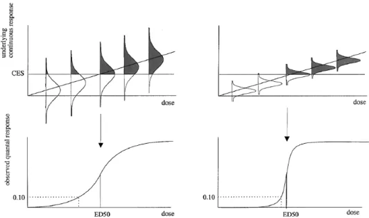
As Figure 1 (from: Slob, 1999) shows, the slope of quantal dose-response data is directly influenced by the variability of the animal population, but also experimental errors, such as dosing errors or remaining heterogeneity in the experimental conditions experienced by each animal. Bokkers et al. (2009) concluded that the slope of the dose-response for quantal data does not provide any information on intra-species variation in humans, and hence the ED50 of the dose-response was regarded as the (only) information useable for further (probabilistic) risk assessment. The ED50 is the dose at which the observed incidence is 50% (without correction for background response). The severity or degree of the effect associated with the ED50 is implicitly defined by the data, i.e. the cut-off between yes/no effect (e.g. mild or minimal lesion). In this interpretation quantal data do not provide any information on severity levels
other than the single one as implicitly defined by the cut-off1.
1 Or, when various severity levels have been scored, the ED50s associated with each severity level could be
Figure 1. Relation between quantal response (e.g., fraction of animals with atrophy; see lower panels) and underlying continuous response (degree of atrophy; see upper panels).
In the left panels of Figure 1 the variation between the individual observations (animal heterogeneity plus experimental error) is relatively large, and in the right panels, relatively small, whereas the average (continuous) dose-response is the same. The (critical) effect size (CES) is the cut-off level above which the experimental observer classifies an animal as having atrophy. Thus, the shaded areas in the distributions reflect the expected percentages of animals considered as responders, which are given in the lower panels as a function of dose. Note that the ED10 moves to the ED50 when the variation between the animals and/or the experimental error is reduced (Slob, 1999).
However, in the case of cancer dose-response data another interpretation of the dose-response relationship is possible. In this second interpretation it is
assumed that each subject may be characterized by a (hypothetical) ‘individual’ dose-response, where the response is the probability that this particular
individual will show cancer at any given dose. The fundamental difference between the two interpretations may be summarized as follows:
Interpretation 1: A specific animal at a specific point in time (i.e. given the history of all circumstances that the animal went through) is characterized by a hypothetical ‘tolerance’ dose. If the animal had been treated with a higher dose, it will show the effect, if it is treated with a lower dose it will not show the effect. Interpretation 2: A specific animal at a specific point in time (i.e. given the
history of all circumstances that the animal went through) is characterized by a hypothetical dose-response relationship. If the animal had been treated with a specific dose, this dose-response determines the probability that the animal will show the effect.
As a further illustration we apply dose X to 100 animals, and at the end of the study we observe that 30% of the animals show cancer. This can be interpreted in two ways:
Interpretation 1: The tolerance doses of 30 specific animals were higher than the applied dose, while those in the other 70 animals were lower. Suppose we could repeat the experiment with the same animals (under identical conditions), then the same individuals would show cancer again.
Interpretation 2: All individual animals had a 30% probability of getting cancer. So, in this respect the animals are identical. If we could repeat the experiment then the group of individuals showing cancer will be different.
In other words, in interpretation 2 the realization of the cancer effect in a single individual is considered as the outcome of a stochastic process, analogous to throwing a coin or a dice. For instance, one might imagine that a single reactive molecule entering the nucleus could hit the DNA, but it is a matter of chance whether it hits a relevant gene or an irrelevant one. If this were (one of the) a critical event(s), then it is also a matter of chance if the animal would develop a tumor or not, given the specific circumstances.
It should be noted that all factors that may influence the carcinogenic process have an impact on the tolerance dose in interpretation 1, and on the cancer probability in interpretation 2.
Although the distinction between the two interpretations seems subtle or even academic, it has a direct impact on how a risk assessment should be worked out. As already discussed, interpretation 1 implies that only the ED50 is useable for further risk assessment. It estimates the dose above which the median human being would get cancer, and below which not (with probability = 1). Hence, in that case, the non-cancer IPRA as worked out for quantal data directly applies to cancer as well (i.e., IPRA based on ED50). However, under
interpretation 2 the fitted dose-response curve could be regarded as an estimate of the mean of all the individual responses. In that case, the
dose-response relationship predicts the probability of getting cancer at any given dose, which may be assumed to hold for the (average) test animal. Next, this relationship may be assumed to equally hold for the average human being (apart from an interspecies dose-factor). So, the ED10 in the animal is (after interspecies scaling) considered as an estimate of an equivalent dose in the median human being, at which he/she will have a probability of 10% of developing cancer. Further, in interpretation 2, a higher dose in the same individual will lead to a larger probability of developing cancer, and this will be regarded as more serious by the individual. In this interpretation higher cancer probabilities may be regarded as increasing severity levels, analogous to more serious degrees of anemia or liver lesions. So, the probability of developing a tumor (in an individual) could be treated as the degree of effect, and a severity level could be associated with any particular value of this probability (e.g., a
tumor probability of 1 per 105 = slight, 1 per 104 = moderate, etc.). Note that
this individual dose-risk relationship is a theoretical notion in the sense that it cannot be experimentally measured: the probability of cancer in a single individual cannot be observed, nor can a single individual be (chronically) exposed to different doses.
The next section discusses various approaches within IPRA that may be applied in the context of a cancer risk assessment. From these, approach B is based on interpretation 1, while approaches C and D are based on interpretation 2. For approach A this distinction is not relevant: it simply takes the BMDL10 as the point of departure, without further interpretation. In approach E the dose-response relationship relates to time-to-tumor, which is a continuous endpoint, so the distinction between the two interpretations neither applies in this approach.
3
Various approaches for using IPRA for carcinogens
This section contains a number of conceptually described potential approaches for using IPRA for carcinogens. Note that this discussion only relates to the hazard characterization part of the IPRA. In all approaches the exposure
assessment part of the IPRA remains the same (see e.g. Van der Voet and Slob, 2007; Van der Voet et al., 2009; Bokkers et al., 2009; Bokkers and Boon, 2010).
3.1 Approach A: MOE applied to cancer
A recently proposed approach for cancer risk assessment is the Margin of
Exposure (MOE; expressed as a ratio)2 between a Point of Departure (PoD, e.g.
Benchmark dose) obtained from the critical dose-response data and the estimated human exposure level (O’Brien et al. 2006; Benford et al., 2010a). This approach can be easily incorporated in an IPRA approach. In line with this ‘deterministic’ MOE approach the tumor incidence dose-response data are used to estimate the BMD10, the dose at which10 % of the animal population is affected. But, while the deterministic MOE approach uses the lower limit of the confidence interval (the BMDL10) as the numerator of the MOE, IPRA uses the complete uncertainty distribution around the BMD10. The distributions for the extrapolation factors, as usually applied in IPRA, will be omitted in this case, analogous to the deterministic MOE. But the variation and uncertainty related to exposure is fully included in the IPRA. This approach of IPRA will result in a distribution of the MOE.
The additional value of applying IPRA is that the uncertainty in the MOE is quantified. This may prevent erroneous conclusions in ranking MOEs associated with different carcinogens, given the current exposure situation. The reason for this is that deterministic MOEs assessed for different substances may differ in the level of conservatism. For instance, one MOE might be based on a very conservative exposure estimate due to lack of data, while another MOE is based on a more realistic exposure estimate in the case that the exposure data are good. This will result in different MOEs, even if the underlying risks are the same. Therefore, simply ranking MOEs without considering the different levels of uncertainties involved may result in unjustified conclusions on relative risks. It should be kept in mind that the MOE approach does not apply inter- and intraspecies factors. Further, the BMD used is usually associated with a cancer risk of 10%. Therefore, MOEs should be much larger than 1 before they could be regarded as ‘no reason of concern’. Attempts have been made to define a MOE reference value, below which there would be ‘no reason of concern’, for instance four orders of magnitude (Barlow et al., 2006). The IPRA concept of IMoE (individual margin of exposure) as used in IPRA below (chapter 3) is
fundamentally different, because it does take inter- and intraspecies differences and their uncertainties into account.
Assumptions:
The MOE can be characterized as an assumption-poor approach. The basic assumption is:
The dose-response in animals is a model for the dose-response in humans. Output:
The IPRA will result in a confidence interval for the MOE, which we define as the
ratio BMD10/E, where E is the 99th percentile of the IEXP distribution. This ratio
is an estimate based on uncertain data, and the confidence interval around it results from both the uncertainties in the exposure data and in the
dose-response data3. The drawback of being assumption-poor is that the output of
this approach is not easy to interpret, in the sense that it remains unclear how any given value of a MOE relates to potential risk levels in the human
population. For instance, the MOE of 10,000 as a reference level for no concern, as proposed by Barlow et al., 2006, has no solid basis, and is an indication at best.
3.2 Approach B: IPRA method for non-carcinogens applied to cancer
Approach B is in fact the existing methodology of IPRA as developed for non-carcinogens (for examples, see Bos et al., 2009; Muri et al., 2009; Müller et al., 2009; Bokkers et al., 2009). This approach is based on interpretation 1. As mentioned in section 2.3, under interpretation 1, the ED50 from a quantal dose-response relationship is the only information that is used in the risk assessment. The assumption is that each individual can be characterized by a tolerance dose, and the ED50 from the animal study is an estimate of the tolerance dose for the median animal. This animal tolerance dose is then scaled (using the interspecies extrapolation factor) to the median human being. Next, it is assumed that individuals differ in the tolerance dose, reflected by the intraspecies distribution. So, the fraction of the population with cancer derives from the intraspecies distribution around the scaled animal ED50.
Assumptions:
1. Quantal data are subject to interpretation 1 (see section 2.3).
2. Potential interspecies differences in sensitivity for the specific chemical between the median animal and median human can be covered by the same uncertainty distribution as for non-cancer. This means that potential differences in sensitivity between test animal and human are assumed to be not fundamentally different for cancer or non-cancer.
Regarding the toxicokinetic4 part of interspecies differences this seems
plausible, for the toxicodynamic5 part this is unclear.
3. In the human population there may be interindividual differences in sensitivity for the specific chemical, i.e. individuals may have different tolerance doses. The assumption is that the variability in human tolerance doses is of the same order of magnitude as the intraspecies
3 Note the difference between variability and uncertainty: Variability is an intrinsic property of a parameter and
is inherent to the system being modeled, whereas uncertainty represents ignorance or partial lack of knowledge and is thus dependent on the current state of knowledge.
4 Toxicokinetics describes the distribution and elimination of the chemical in the body, resulting in the internal
dose at the tissue level.
5 Toxicodynamics describes the interaction of the substance with the target tissue, resulting in the biological
variation for non-cancer effects. Again, for toxicokinetic differences this might be a plausible assumption, while for toxicodynamic differences it has been argued that inter-individual human variability in cell cycle control and DNA repair would result in additional intraspecies variation as compared to non-cancer effects (Barlow et al. 2006). The latter assumption could be taken into account in any specific application of IPRA, if considered appropriate.
4. The fraction of the IMoE distribution with IMoE below 1 is interpreted as the fraction of the population that will develop cancer (after lifelong exposure).
Output:
The output of approach B is comparable to the IPRA output for non-cancer effects:
1. The fraction of individuals with an exposure exceeding their own individual tolerance dose (analogous to critical effect dose for non-cancer effects), i.e. the dose where the individual would develop non-cancer. For risk managers such output would only be helpful if that fraction is sufficiently low. While theoretically very low fractions can be calculated in IPRA, the problem is that they largely depend on the intraspecies distribution, which is in fact an assumed distribution with very little (quantitative) support from data.
2. The individual margin of exposure (IMoE) for a chosen (e.g. 1st)
percentile of the population. It should be noted here that the IMoE approach is, in the current software, based on Monte Carlo calculations, so that the estimated fraction of the population is limited by the number of Monte Carlo runs. For instance, when the number of runs is chosen to be one million, risk below than one in a million are beyond reach. In interpreting the estimated IMoE, the seriousness of the effect could be taken into account in a semi-quantitative way: a more serious effect
would call for a larger IMoE, and hence for cancer the 1st percentile of
the IMoE distribution should normally be substantially larger than 1 before it could be concluded that there is ‘no reason of concern’,
analogous to the deterministic MOE. How much larger is hard to say, but not as much as for the MOE of approach A because inter- and
intraspecies differences are already accounted for in the IMoE.
3.3 Approach C: Linear extrapolation
Next to the MOE approach (approach A) another current method in risk assessment of carcinogens is that of linear extrapolation, and this forms the basis of approach C. In linear extrapolation, a straight line is ‘drawn’ from the dose with an observable tumor incidence (the PoD) to the tumor incidence in the controls, with the aim to obtain the dose at which a low, acceptable (but
unobservable) incidence would occur. Note that approach C (just as approach D, see section 3.4) is based on interpretation 2 of the dose-response data.
In this study the linear extrapolation approach is worked out in the IPRA
philosophy as follows. A series of models is fitted to the dose-response data and for those models that fit the data sufficiently well the BMD10 is assessed, together with an uncertainty distribution (using bootstrapping). The bootstrapped uncertainty distributions are joined to one overall uncertainty
distribution for the BMD10. The distribution for doses at lower risk levels is then simply obtained by dividing the distribution by the relevant factor (e.g., for risk 1 per 1000 this factor is 100, which is the ratio of 1 per 10 to 1 per 1000). For each of the BMD distributions obtained (i.e. related to various nominal risk levels) the IPRA can be applied in the usual way.
Assumptions:
1. Tumor incidence data are subject to interpretation 2 (see section 2.3). In this interpretation different ‘degrees’ of developing cancer can be defined, i.e. in terms of the probability that it will actually happen (in a given individual). Therefore, the IMoE distribution can be estimated for any ‘severity’ level, where a low/high severity level is a small/large cancer risk (in a given individual).
2. Assumption on interspecies uncertainty: the same as approach B. 3. Assumption on intraspecies variation and uncertainty: the same as
approach B, but intraspecies variation is now defined as variation in human equipotent doses, i.e. individual doses associated with the same cancer probability.
4. The fraction of the IMoE distribution with IMoE below 1 is interpreted as the fraction of the population the individuals of which have a given (specified) probability of developing cancer due to the exposure of the carcinogen considered.
Output:
The typical output is the same as in approach B (i.e. in terms of the IMoE for the
1st percentile of the population, or in terms of an estimated fraction of the
population) but now these outcomes can be calculated for various risk levels, where risk is interpreted as the degree of the effect (in terms of cancer risk) that an individual would be subject to. As a result, risks are expressed in two dimensions: a fraction of the population, and the cancer risk associated with the individuals in that fraction of the population. For example: 2% of the population has a cancer risk of 1:10,000.
In all cases the output is accompanied with the associated uncertainties (confidence intervals).
3.4 Approach D. Model extrapolation (and model-averaging)
Approach D differs from approach C in the way of low-dose extrapolation: instead of linear extrapolation, extrapolation from a fitted model is performed, or rather, from a series of fitted models that were found to result in a
reasonable fit. The variation in outcomes between different models will tend to increase with smaller risk levels, due to the fact that an increasing extent of extrapolation is involved. So, in this approach, the ‘model uncertainty’, which will be large for low risks, is taken into account. For an illustration, see Table 1 (upper part), where, over a series of fitted models the minimum of the BMDLs and the maximum of the BMDUs are reported. These results relate to typical carcinogenicity dose-response data (see Figure 2). The ratio
max(BMDU)/min(BMDL) is given in Table 1 as a measure of uncertainty (a high ratio means a large difference between BMDU and BMDL and therefore a high uncertainty). This illustrates that the uncertainty in the BMD estimate rapidly increases with smaller risk levels.
The advantage of approach D over linear extrapolation (approach C) is that it provides a more realistic confidence interval for the dose at a given (low) risk, because it takes model uncertainty into account. The width of this confidence
interval will depend on the quality of the data. As an illustration, compare the uncertainty ratios for a large study using 2280 animals for NDMA (Peto et al., 1991a, b), summarized in Table 2, with those in Table 1: the ratios are much smaller for the study with the large number of animals and doses.
For a given severity level (e.g. cancer risk = 1 per 104), the confidence interval
around the BMD resulting from approach D can be compared to the result from linear extrapolation (approach C). If the confidence interval of approach D includes doses much higher than those resulting from approach C, this indicates that the estimates from linear extrapolation method were probably conservative. So, by comparing the results of the two methods it becomes visible to what extent linear extrapolation might be conservative (for a further illustration of this idea, see Figure 2. The latter depends on the quality of the data, although it should be noted that data as those underlying Table 2 are rare in practice. Just as described for linear extrapolation (approach C), the overall uncertainty associated with the BMD is quantified by joining the individual bootstrap distributions (related to different models). This implies that all accepted models receive equal weight. It would probably be better to join the individual
distributions by giving weights based on the log-likelihood associated with each model, analogous to model averaging approaches (e.g., Wheeler and Bailer, 2007, 2008). The latter has not yet been implemented in the IPRA software. Assumptions
1. Tumor incidence data are subject to interpretation 2 (see section 2.3). In this interpretation different ‘degrees’ of developing cancer can be defined, i.e. in terms of the probability that it will actually happen (in a given individual). Therefore, the IMoE distribution can be estimated for any ‘severity’ level, where a low/high severity level is a small/large cancer risk (in a given individual).
2. It is assumed that the ‘true’ dose-response is (close to) one of the curves resulting from fitting the usual suite of models to the data. 3. See approach C.
4. See approach C. 5. See approach C.
6. The models are fitted with the shape parameter constrained such that the slope at dose zero if finite. The underlying assumption is that a linear low-dose response relationship is worst-case in the case of genotoxic carcinogens.
Output:
Obviously, the uncertainties calculated in approach D will be larger than in approach C, since this approach aims to take into account all possible shapes for the dose-response curve, rather than just a linear shape below the BMD10. See also Figure 2.
The output can be represented in two different forms.
1. Similar as described in Approach C, i.e. results for various fixed levels of risks.
2. The overall expected fraction of the population with cancer. See Appendix C for the computational details.
Table 1. Minimum BMDL and maximum BMDU for the models available in PROAST fitted to the data in Figure 2.
extra risk 1 per 10 1 per 103 1 per 104 1 per 105
min(BMDL) 1.14 0.0118 0.00118 0.000118
max(BMDU) 4.02 1.04 0.722 0.526
ratio max/min 3.5 88 612 4458
Table 2. Minimum BMDL and maximum BMDU for the models available in PROAST fitted to liver tumors in the NDMA study (Peto et al., 1991a,b), which used 2280 animals and 16 dose groups.
extra risk 1 per 10 1 per 103 1 per 104 1 per 105
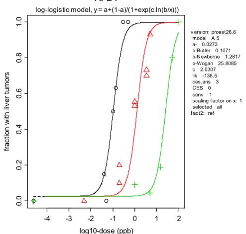
min(BMDL) 0.0291 0.000442 0.0000444 4.44E-06 max(BMDU) 0.0503 0.00859 0.00701 0.00334 ratio max/min 1.7 19 158 752 0 5 10 15 20 25 30 0. 0 0. 2 0. 4 0. 6 0. 8 1. 0 das4 dose.kg.bw fo re st om ac h log-logistic in terms of BMD v ersion: Proast24.12 model A 18 a- 0.0119 BMD-1 2.4533 BMD-2 3.4118 c 2.5724 lik -110.93 b: 5.764 b: 8.015 ces.ans 3 CES 0.1 conv 1 scaling f actor on x: 1 selected all f act2: sex extra risk 0.1
Figure 2. Dose-response data used for Table 1, together with fitted log-logistic model. Triangles: males: circles: females.
3.5 Approach E. Time-to-tumor
For various reasons, both theoretical and practical, time-to-tumor data (i.e. data that describe the time it takes to develop a tumor in each individual animal) would form a better starting point for cancer risk assessment than using tumor-incidence data as considered in the four previous methods. Such data are however scarce, and in many cases hard to generate: in many tissues the tumors are only visible after section.
A theoretical option would be to estimate the time-to-tumor dose-response from tumor incidence data, by considering a specific type of models (the ‘latent
variable’ models, LVMs) available in the PROAST software (see Appendix A). This approach appears to be not practically applicable, given the limited information available in typical dose-tumor incidence data. Therefore, as yet, the time-to-tumor approach could only be used if time-to-time-to-tumor has actually been measured. In these (rare) cases, IPRA can be based on an analysis of these data, in the same way as for non-cancer data. It should be noted here that the benchmark response (BMR) for the response ‘time-to-tumor’ would be at least around 5% (to avoid extrapolation), which would probably considered as a severe effect: if the tumor were lethal, this would imply a 5% reduction in lifespan. Nonetheless, extrapolation to lower BMRs involves a smaller low-dose extrapolation step than the usual step needed for tumor incidences (e.g. from 1
per 10down to 1 per 106, which is five orders of magnitude). This would
constitute one of the advantages of using time-to-tumor data.
3.6 Summary of the differences between the five approaches
Table 3 summarizes the differences between the five approaches. The
uncertainty and variability in the dietary exposure is completely included in all five approaches in the same way. The inter- and intraspecies differences are fully taken into account in all approaches, except approach A. The interpretation of the dose-response data (tolerance dose vs. stochastic process) is not relevant for approaches A and E, while approach B (tolerance-dose) differs in this aspect from approaches C and D (stochastic process). The five approaches particularly differ in the PoD that is used. Finally, the uncertainties in the dose-response data are taken into account by a full uncertainty distribution for the PoD in all five approaches.
Table 3. Summary of the five approaches Approach Uncertainty /variability in exposure Inter- and intraspecies extrapolation Inter-pretation Point of Departure Uncer-tainty in PoD A: MOE + - - BMDx (x=10% risk) distr B:
non-cancer + distr 1 ED50 distr
C: linear extrapol. + distr 2 BMDx x=risk level distr D: model extrapol. + distr 2 BMDx x=risk level distr E: time-to-tumor (TTT) + distr - BMDx x=percent reduction in TTT distr
+ : fully taken into account - : not applicable
4
Case study: aflatoxin B1
We considered aflatoxin B1 as the model chemical for illustrating the various
options for a carcinogenic IPRA. This chemical was also included in Boon et al. (2009), which discussed the risk assessment of dietary exposure to
contaminants and pesticide residues in young children in the Netherlands. The MOE (margin of exposure) was found to be somewhat lower than 100, similar to the value found in O’Brien et al. (2006) for the general (adult) population. This low value would be a reason of concern according to EFSA (Barlow et al., 2006), and thus a higher-tier probabilistic assessment is appropriate.
4.1 Exposure assessment
The exposure characterization was performed using the same data and methods as described in Boon et al. (2009). For a detailed description of the exposure characterization the reader is referred to that report. Here we report the summary results of the exposure assessment for children, aged 2 to 6 year (Table 4). Note that the same exposure data were used in all IPRA approaches discussed.
Table 4. Summary data of the intake of aflatoxin B1 by children (age 2-6 y)
Percentiles of exposure (ng/kg bw/d) P50 P95 Aflatoxin B1 exposure (95% CI) 0.8 (0.6-0.9) 1.9 (1.5-2.5) 4.2 Dose-response analysis
Several investigators have studied the carcinogenic potential of aflatoxins in vivo using laboratory animals. The principal tumors induced were liver tumors (IARC, 2002; JECFA, 1998).
The PROAST software6 was used to apply response modeling to the
dose-response data on liver tumors observed in three different studies: Newberne (1965), Wogan et al. (1974), and Butler and Barnes (1968). In fitting dose-response models, the data from these three studies were combined (with study as a covariate regarding the potency parameter b). As an illustration Figure 3 shows a dose-response derived from the data of the three studies. Here the log-logistic model is applied to describe the data from Butler and Barnes, 1968 (left curve and circles), Newberne (1965) (middle curve and triangles), and Wogan et al. (1974) (right curve and plus-signs). Only the study by Wogan et al. (1974) is considered relevant for risk assessment, as the other two studies did not apply chronic exposure (O’Brien et al., 2006). These two studies are merely used as additional information on the shape of the dose-response (the statistical analysis showed that the three studies can be described by the same curve with only parameter b differing among studies).
In the Wogan study groups of male Fischer rats (initial number unspecified) were fed a diet containing 0, 1, 5, 15, 50 or 100 µg aflatoxin B1/kg of diet. These feed concentrations corresponded to doses of 0.05, 0.1, 0.3, 2 and 4 µg/kg bw/d, respectively (assuming default body weight male rats 500 g and default feed consumption male rats 20 g/d; O’Brien, 2006). When clinical
deterioration of animals was observed all survivors in that treatment group were killed. The incidences of hepatocellular carcinomas are reported in Table 5.
-4 -3 -2 -1 0 1 2 0. 0 0.2 0. 4 0.6 0. 8 1.0
AFB1
log10-dose (ppb) fr ac tio n w ith li ve r tu m or s v ersion: proast26.6 model A 5 a- 0.0273 b-Butler 0.1071 b-Newberne 1.2817 b-Wogan 25.8085 c 2.0307 lik -136.5 ces.ans 3 CES 0 conv 1 scaling f actor on x: 1 selected all f act2: reflog-logistic model, y = a+(1-a)/(1+exp(c.ln(b/x)))
Figure 3. Dose-response data of liver tumor incidence against the log10 dose (ppb). The curves obtained with the log-logistic model are shown as an illustration. Data are from Butler and Barnes, 1968 (triangles),
Newberne, 1965 (circles, two circles per dose indicates male and female data), and Wogan et al., 1974 (plus symbols).
Table 5. Incidences of liver tumors in male rats after prolonged exposure to various doses of aflatoxin B1 (Wogan et al., 1974).
Dose (ppb) No. animals with
liver tumor Group size 0 0 18 1 2 22 5 1 22 15 4 21 50 20 25 100 28 28
Appendix B summarizes the results for the usual suite of models (e.g. EFSA, 2010) fitted to the liver tumor incidence data. Seven of the nine models were accepted by the goodness-of-fit test for p>0.01, and therefore all these models were included in deriving the uncertainty distributions for the various BMDs used.
The BMD distributions were derived by the parametric bootstrap method, i.e. by generating datasets from the fitted model, refitting the model to the artificial data and recalculating the BMD in each run (number of runs = 1000). This was repeated for each of the models accepted by the data. The distributions of the
‘bootstrapped’ BMDs are summarized in Table 6 by their lower 5th (BMDL) and
upper 95th (BMDU) percentiles. BMD distributions were derived for consecutively
increasing steps in extra risk from 1 per 10 up to 1 per million, denoted as 1e-1 to 1e-6, respectively. In addition the ED50s (= dose at 50% incidence) with their confidence intervals were estimated for each model (except for the Gamma model, for which estimation of the ED50 is not implemented in the PROAST software).
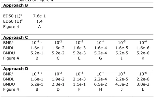
The BMDs and ED50s in ppb are translated into μg/kg bw/day by multiplying the values in ppb by 0.04, according to O’Brien (2006). The distributions obtained for each model were combined to obtain an overall BMD uncertainty distribution (Table 6 and Figure 4). The diverging BMD distributions from the individual models result in multimodal BMD distributions, especially for lower extra risks. Table 6 also shows the BMD distributions for various risk levels as derived by linear extrapolation from the BMD10 distribution.
Table 6. Summary of the BMD and ED50 distributions obtained with all seven accepted models, combined. BMD(L/U)s are in µg/kg bw/d. Graphical representations of the distributions are given in the corresponding panels of Figure 4. Approach B ED50 (L)c 7.6e-1 ED50 (U)c 1.4 Figure 4 A Approach C BMRa 10-1b 10-2 10-3 10-4 10-5 10-6
BMDL 1.6e-1 1.6e-2 1.6e-3 1.6e-4 1.6e-5 1.6e-6
BMDU 5.2e-1 5.2e-2 5.2e-3 5.2e-4 5.2e-5 5.2e-6
Figure 4 B C E G I K
Approach D
BMRa 10-1b 10-2 10-3 10-4 10-5 10-6
BMDL 1.6e-1 1.9e-2 2.1e-3 2.2e-4 2.2e-5 2.2e-6
BMDU 5.2e-1 2.0e-1 1.1e-1 6.5e-2 4.3e-2 3.0e-2
Figure 4 B D F H J L
a defined as extra risk
b For BMR = 10%, results for approaches C and D are identical c L = lower bound, U = upper bound estimate
(A) BMR = ED50, approach B
log10 ED50 (ug/kg bw /dy)
F re que nc y -0.3 -0.2 -0.1 0.0 0.1 0.2 0.3 0 500 10 00 150 0
(B) BMR = 1e-1, approach C & D
log10 BMD (ug/kg bw /dy)
F re que nc y -1.0 -0.8 -0.6 -0.4 -0.2 0 200 400 600 (C) BMR = 1e-2, approach C
log10 BMD (ug/kg bw /dy)
F reque nc y -2.0 -1.8 -1.6 -1.4 -1.2 0 200 400 60 0 (D) BMR = 1e-2, approach D
log10 BMD (ug/kg bw /dy)
F reque nc y -2.0 -1.5 -1.0 -0.5 0 200 60 0
(E) BMR = 1e-3, approach C
log10 BMD (ug/kg bw /dy)
F requ enc y -3.0 -2.8 -2.6 -2.4 -2.2 0 200 400 60 0 (F) BMR = 1e-3, approach D
log10 BMD (ug/kg bw /dy)
F requ enc y -3.0 -2.5 -2.0 -1.5 -1.0 -0.5 0 40 0 800 120 0 (G) BMR = 1e-4, approach C
log10 BMD (ug/kg bw /dy)
Fr eq ue nc y -4.0 -3.8 -3.6 -3.4 -3.2 0 200 400 600 (H) BMR = 1e-4, approach D
log10 BMD (ug/kg bw /dy)
Fr eq ue nc y -4.0 -3.5 -3.0 -2.5 -2.0 -1.5 -1.0 -0.5 0 40 0 800
(I) BMR = 1e-5, approach C
log10 BMD (ug/kg bw /dy)
F req ue nc y -5.0 -4.8 -4.6 -4.4 -4.2 0 200 400 60 0 (J) BMR = 1e-5, approach D
log10 BMD (ug/kg bw /dy)
F req ue nc y -5 -4 -3 -2 -1 0 500 15 00 (K) BMR = 1e-6, approach C
log10 BMD (ug/kg bw /dy)
F req ue nc y -6.0 -5.8 -5.6 -5.4 -5.2 02 00 40 0 60 0 (L) BMR = 1e-6, approach D
log10 BMD (ug/kg bw /dy)
F req ue nc y -6 -5 -4 -3 -2 -1 0 500 15 00
Figure 4. Uncertainty distributions for ED50 and BMDs (µg/kg bw/d) associated with various BMRs obtained by combining the bootstrap results from all seven accepted models.
As expected, the width of the distributions, i.e., the uncertainty in the BMD, increases with lower extra risk levels when model uncertainty is taken into account (see plots headed ‘model extrapol’), while the distributions remain narrow when linear extrapolation is applied. This is caused by the fact that the upper bounds are much higher in ‘model extrapolation’. The lower bounds of the distributions are similar between ‘model extrapolation’ and ‘linear extrapolation’. The latter is related to the fact that in ‘model extrapolation’ the models were constrained to have finite slope at dose zero, which effectively means that from all dose-response shapes allowed in the analysis, the linear shape (at low doses) is the worst case shape. See Figure 5 for a further illustration.
dose fr a cti o n w ith e ffe ct 1 10 100 0 .01 0. 1 1 BMR <— 0 BMD <— 0
Figure 5. Illustration of the fact that the lower confidence limit for the BMD at lower risks for approach D (model extrapolation) is similar to that for approach C (linear extrapolation), while the upper bound for approach D may by much higher than for approach C. Approach D allows dose-response curves such as the two dashed curves, reflecting two possible dose-response relationships that are compatible with the observed responses, but differ widely at lower risks levels. However, they remain at the right side of the straight line, which reflects linear extrapolation.
4.3 Extrapolation factors
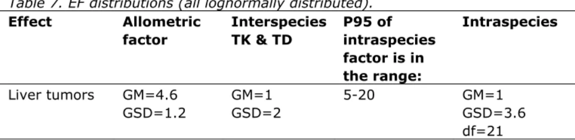
The animal derived BMD distributions are extrapolated to the human population using an interspecies and intraspecies extrapolation factor (EF). Table 7 gives an overview of the EF distributions that were applied in this aflatoxin case study. Interspecies extrapolation is performed in two steps:
1. allometric scaling to account for interspecies differences in body size 2. applying an EF for interspecies differences in kinetics and dynamics
To achieve allometric scaling the following factor was applied: power scaling
bw
animal
mean
bw
human
mean
1,
where the mean human bw is set at 80 kg and the mean male rat bw at 500 g (O'Brien et al., 2006). The allometric scaling power is assumed to be in the range of 0.65 to 0.75. To account for this uncertainty, the scaling power is described by a (normal) distribution with a mean of 0.7 and SD of 0.033. This
SD follows from assuming that the 5th and 95th percentiles of the distribution are
0.65 and 0.75, respectively. These assumptions translate into a lognormal distribution for the allometric factor with GM = 4.6, and GSD = 1.2. Table 7. EF distributions (all lognormally distributed).
Effect Allometric factor Interspecies TK & TD P95 of intraspecies factor is in the range: Intraspecies Liver tumors GM=4.6 GSD=1.2 GM=1 GSD=2 5-20 GM=1 GSD=3.6 df=21 GM: geometric mean
GSD: geometric standard deviation
For potential toxicokinetic and toxicodynamic differences between rat and
human the usual EFinterspecies distribution was used (Bokkers and Slob, 2007;
Bokkers et al., 2009), i.e. GM = 1 and GSD = 2.
The variability in sensitivity within the whole human population is accounted for by an intraspecies EF. In IPRA this variability is based on expert judgment,
expressed in terms of a factor between the 50th and 95th (P95) percentile of the
human sensitivity distribution, reflecting by how much the individual BMD of the sensitive 5% of the population might be lower than that of the average (= median) individual. Since this factor itself is uncertain, an assumption is made about the range of potential values; in this case it is assumed that this factor lies somewhere between 5 and 20. This (uncertain) information can be translated into a lognormal distribution with GM = 1 and GSD = 3.6 for reflecting the variability, and an associated chi-squared distribution of 21 degrees of freedom for the GSD, reflecting the uncertainty in the assumed variability. For a detailed description of the construction of the intraspecies EF, see Van der Voet et al. (2009).
4.4 Probabilistic risk assessment
Approach A
The 1st percentile of the distribution of the MOE (ratio BMD
10/IEXP) was found to
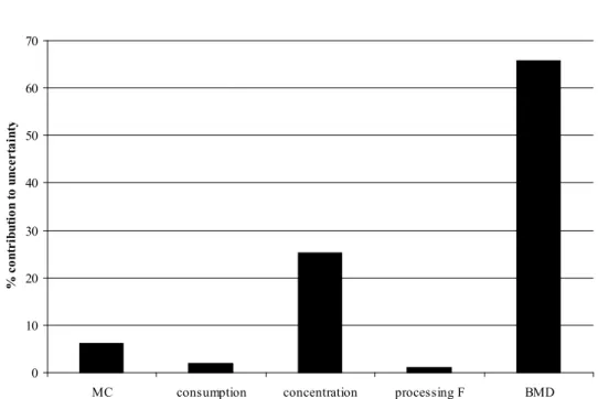
be somewhere between 24 and 102 (90%-confidence interval), i.e., 99% of the population would have an MOE larger than that (see Table 8). Around 65% of the uncertainty in this value was attributable to uncertainty in the BMD10, and around 25% to uncertainties in the concentration data (see Figure 6).
Table 8. Results for approach A.
1st percentile of MOE distribution
BMR
L05 L95
1e-1 24 102
L05: 5% lower confidence bound L95: 95% upper confidence bound
0 10 20 30 40 50 60 70
MC consumption concentration processing F BMD
% co nt ri bu ti on to u ncert ai nt y
Figure 6. Contribution of various sources of uncertainty (Monte Carlo,
consumption data, concentration data, processing factor and BMD) to the overall uncertainty associated with the 1st percentile of the MOE
distribution.
Approaches B, C, and D
As opposed to approach A, approaches B, C and D do apply distributions for assessment factors. Further, for these three approaches the usual output from IPRA can be produced, i.e. (i) in the form of confidence intervals for the
individual margin of exposure (IMoE) associated with the 1st percentile of the
population, and (ii) in the form of the fraction of the population with an exposure that is higher than his/her personal dose associated with a given degree of effect. The first type of output is shown in Figure 7 and Table 9, the second in Figure 8 and Table 10.
Approach B
If cancer dose-response data (where response is in terms of incidences) are interpreted in the same way as quantal data for non-cancer (interpretation 1, see section 2.3) then approach B applies, where the hazard characterization is based on the ED50. Since the upper confidence interval in Figure 7 is larger than one (or zero on the log-scale used) this indicates that 99% of the population
would not get cancer from aflatoxin B1 exposure. However, since the lower
confidence bound of the IMoE for the 1st percentile of the population is quite
close to one, this indicates that the fraction of the population that would get cancer might not be much smaller than 1%. This is more precisely shown in Table 10: the upper confidence limit of the fraction of the population with cancer is 0.55%. Such a result might have been interpreted as sufficiently protective by risk managers in the case of many non-cancer effects, such as mild
histopathological lesions. However, since cancer is considered to be a much more serious effect than mild histopathological lesions, the statement that 99.45% of the population would not get cancer might not satisfy risk managers. Approach C and D
Approaches C and D are based on the second interpretation of the tumor
incidence data (see section 2.3), i.e., the observed incidences are interpreted as individual risks. In that case doses at lower risks can be estimated based on the observed dose-response in animals. In approach C this is done by linear
extrapolation from the BMD10 (upper part of Figures 7 and 8), while in approach D this is done by extrapolating from the various models that were found to be compatible with the data (lower part of Figures 7 and 8). As an example,
consider the 4th confidence interval from the bottom of Figure 7. Here, the
complete confidence interval for the 1st percentile of the IMoE distribution
related to a 10-3 risk is below 1 (= 0 on log-scale). This implies that the persons
in the 1st percentile of the population would have a cancer risk of at least 1 in
1000 (=10-3 or 1e-3). Note that the relatively high risk in these individuals may
be due to a relatively high exposure and/or due to being relatively sensitive to
aflatoxin B1 (i.e., at a given exposure they would have a higher cancer risk than
the average sensitive person).
Figure 8 shows another way of summarizing the results: in terms of the
estimated fraction of the population that would have a particular cancer risk. For instance, the fraction of the population that would have a cancer risk of 1 in 100 (or lower) is somewhere between 0.34% and 31% according to approach D, and somewhere between 0.77% and 34% according to approach C (see Table 10).
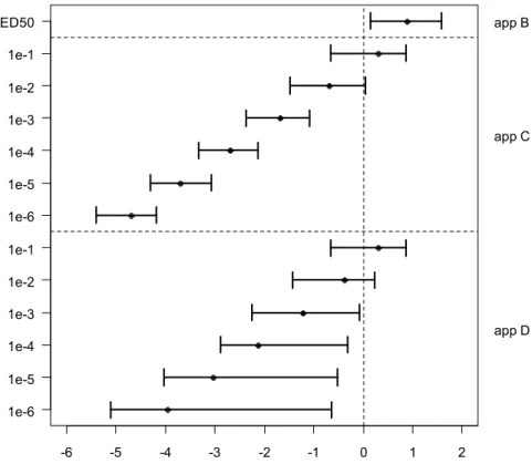
log10 1st percentile of the IMoE distribution -6 -5 -4 -3 -2 -1 0 1 2 1e-6 1e-5 1e-4 1e-3 1e-2 1e-1 1e-6 1e-5 1e-4 1e-3 1e-2 1e-1 ED50 app D app C app B
Figure 7. The 1st percentile of the IMoE (=ICED/IEXP) distribution (on log 10
scale), given as 90%-confidence intervals. Left axis: individual cancer risk; right axis: IPRA approach B, C (linear extrapolation) or D (model extrapolation).
Table 9. Confidence intervals for the 1st percentile of the IMoE distribution
1st percentile of IMoE distribution
BMR P05 P95 P05 P95 Approach B 1.4 38 Approach D Approach C BMR (extra risk) 10-1 (10%) 0.22 7.3 10-2 (1%) 3.8e-2 1.7 3.3e-2 1.1
10-3 5.7e-3 0.85 4.2e-3 8.3e-2
10-4 1.3e-3 0.49 4.7e-4 7.3e-3
10-5 9.4e-5 0.30 5.0e-5 8.5e-4
10-6 7.9e-6 0.23 4.0e-6 6.5e-5
% population with IMoE<1 <0.0001 0.001 0.1 1 10 50 90 >99.99 1e-6 1e-5 1e-4 1e-3 1e-2 1e-1 1e-6 1e-5 1e-4 1e-3 1e-2 1e-1 ED50 app D app C app B
Figure 8. The percentage of the population with IMoE < 1 (i.e. IEXP > ICED). Dots are the best estimates and whiskers represent the 90% confidence interval. The x-axis is on logit-scale, to improve visibility of extreme fractions. Left axis: individual cancer risk; right axis: IPRA approach B, C (linear extrapolation) or D (model extrapolation). The confidence intervals reflect the fraction of the population for which the cancer risk is smaller than or equal to the value given at the y-axis.
Table 10. Confidence intervals for the fraction (%) of the population with IMoE < 1
Fraction (%) of population with IMoE < 1 BMR P05 P95 P05 P95 Approach B <1.0e-4* 0.55 Approach D Approach C BMR (extra risk) 10-1 (10%) 8.0e-3 6.9 10-2 0.34 31 0.77 34 10-3 1.3 79 23 87 10-4 2.3 98 80 100 10-5 5.4 100 98 100 10-6 8.6 100 100 100
P05 and P95: 5% lower and 95% upper confidence bounds
* Lower risks could not be calculated because the number of Monte Carlo runs used was one million here.
The results from approach D as summarized in Table 10 and Figure 8 are rather complex, and for risk management purposes it would be helpful to simply have an estimate of the expected fraction in the overall population with cancer. The procedure of how to calculate this is summarized in Appendix C.
For the aflatoxin B1 case this resulted in a 90%-confidence interval (two-sided)
of 0.009% to 1.8%.
4.5
Relative contribution of sources of uncertainty
Figure 9 shows the relative contribution of various sources of uncertainty to the
1st percentile of the IMoE distribution. These results show some striking
features. First of all, the uncertainties related to exposure hardly contribute at all in all approaches. It may be noted that in this case the exposure information is relatively good, although the concentrations are likely positively biased due to targeted sampling (Boon et al. 2009). Further, in an IPRA based on the ED50 or BMD10 the uncertainty is dominated by interspecies extrapolation. This also holds for approach C (linear extrapolation). But in approach D the uncertainty in the BMD is by far the largest contributor, making the other uncertainties
relatively unimportant.
4.6 Comparing IPRA results with simple linear extrapolation
It is interesting to compare the results from the IPRA approaches B and
D with the simple linear extrapolation method as currently applied in
various countries and organizations. Based on the lowest BMDL10 of 3.3
ppb (see Appendix B), which is equivalent to 132 ng/kg bw, and the
median exposure estimate of 0.8 ng/kg bw for children (age 2-6 y; see
table 4) the simple linear extrapolation method results in a risk (point
estimate) of 0.061%.
IPRA approach B resulted in a 90%-confidence intervals for the expected
fraction of the population with cancer with an upper bound of 0.55%
(see Table 10), while approach D resulted in an upper bound of 1.8%
(see end of section 4.3). Both these values are higher than the point
estimate from the classical linear extrapolation. This is due to the fact
that the simple linear extrapolation method does not take inter- and
intraspecies differences into account. The latter was confirmed by
calculating the confidence interval for risk using approach D, but with
both extrapolation factors omitted: in that case the upper bound was
very close to the point estimate from classical linear extrapolation.
These results illustrate the problem that simple linear extrapolation as
currently applied by some countries does not allow for potential inter-
and intraspecies differences. It is sometimes argued that the latter
differences are already accounted for by the fact that linear
extrapolation is conservative. However, such arguments make the
procedure highly non-transparent. In IPRA potential inter- and
intraspecies differences are fully taken into account.
0 10 20 30 40 50 60 70 MC consumption concentration processing F BMD interspecies F intraspecies F % contribution to uncertainty 0 10 20 30 40 50 60 70 MC consumption concentration processing F BMD interspecies F intraspecies F % contribution to uncertainty
BMR = ED50 (approach B) BMR = 1e-1 (approach C/D)
0 10 20 30 40 50 60 MC consumption concentration processing F BMD interspecies F intraspecies F % contribution to uncertainty 0 10 20 30 40 50 60 70 MC consumption concentration processing F BMD interspecies F intraspecies F % contribution to uncertainty
BMR = 1e-3 (approach C) BMR = 1e-6 (approach C)
0 20 40 60 80 100 MC consumption concentration processing F BMD interspecies F intraspecies F % contribution to uncertainty 0 20 40 60 80 100 MC consumption concentration processing F BMD interspecies F intraspecies F % contribution to uncertainty
BMR = 1e-3 (approach D) BMR = 1e-6 (approach D)
Figure 9. Contribution of various sources of uncertainty (intra- and interspecies extrapolation, BMD, processing factor, concentration data, consumption data, Monte Carlo) to the overall uncertainty associated with the 1st
Figure 10. Summary of estimated risks for aflatoxin B1. The lines represent the
confidence intervals for risk resulting from the various methods. The lower plot zooms in on the right part of the x-scale.
Lin.extrap.: the classical linear extrapolation method;
Approach D, no EFs: same as approach D, but with inter- and intraspecies extrapolation factor omitted;
Approach D, less potent: a virtual chemical, based on aflatoxin B1, but
with potency 1000-fold lower (see section 5 for a further discussion).
-20 -15 -10 -5 0 log10 of risk (%) lin.extrap approach B approach D approach D no EFs approach D less potent -4 -3 -2 -1 0 1 log10 of risk (%) lin.extrap approach B approach D approach D no EFs approach D less potent