a) RIVM, Bilthoven
b) Alterra, Wageningen
*) Corresponding author. Email ton.van.der.linden@rivm.nl
RIVM report 716601009/2004
Dutch Environmental Indicator for Plant Protection Products
Description of input data and calculation methods A.M.A. van der Lindena,*, J.W. Deneerb, R. Luttika, R.A. Smidtb
This investigation has been performed by order and for the account of the Ministry of Spatial-planning, Housing and the Environment within the framework of project M/716601, ‘Pesticide Fate in the Environment’. The Alterra contribution has been performed by order and for the account of the Ministry of Agriculture, Nature and Food Quality within the framework of research program 416 ‘Pesticides and the Environment’.
Het rapport in het kort
Nationale MilieuIndicator voor gewasbeschermingsmiddelen; Beschrijving van concepten en invoergegevens
De Nationale MilieuIndicator (NMI) voor gewasbeschermingsmiddelen is een softwarepakket dat wordt gebruikt voor de berekening van emissies en milieubelasting van deze middelen. Het pakket kan worden ingezet voor berekeningen op regionale en nationale schaal, voor onder andere de MilieuBalans en Emissie-Registratie. Een uitgebreide toepassing van het pakket is voorzien in de evaluatie van het gewasbeschermingsbeleid voor de periode 2001 – 2010. Dit rapport geeft een beschrijving van benodigde invoergegevens van het softwarepakket en de concepten van de gebruikte berekeningswijzen.
Trefwoorden: bestrijdingsmiddelen; duurzame gewasbescherming; indicatoren; milieubelasting
Abstract
Dutch Environmental Indicator for Plant Protection Products; Description of input data and calculation methods
The Dutch Environmental Indicator for plant protection products (NMI) is a software package used for calculating the potential environmental impact of plant protection products, which are used in agriculture. The software package can be used for calculations at the regional and national scale, amongst other for calculations for the Environmental Balance of the Netherlands and the Emission Registration. It is foreseen that the software package will be used in the evaluation of the current policy on plant protection products. This report gives an overview of input data and calculation procedures used to estimate the emissions and potential impacts of these products.
Preface
In this report the Dutch Environmental Indicator for plant protection products is referred to as NMI, which is an acronym for Nationale MilieuIndicator: the Dutch name of the software package.
The work described in this report has been discussed several times with representatives of the Dutch ministries of LNV and VROM and other stakeholders. We are grateful for constructive discussions and appreciated the suggestions for improvements. The group of representatives consisted most recently of (alphabetical order):
André Bannink, VEWIN Dominique Crijns, VROM Jan Duijzer, TNO
Rob Faasen, RIZA Hans de Graaf, CML Olaf Hietbrink, LEI Gerty Horeman, LNV-EC Jan Huijsmans, A&F Paul Jellema, PD Marianne Mul, UvW Jo Ottenheim, LTO
Michelle Talsma, STOWA Jurgen Vet, Nefyto
Peter van Vliet, CTB Erna van de Wal, CML Frank Wijnands, PPO
Contents
Samenvatting 7 Summary 9 1 Introduction 11 1.1 Overview of indicators 11 1.2 General principles 121.3 Running the system, input and output 12
1.4 Set-up of the report 13
2 Input data 15
2.1 GIS components 15
2.2 Soil data 15
2.3 Climate data 15
2.4 Crops 16
2.5 Plant protection product use data 16
2.6 Application techniques 17
2.7 Crop interception 18
2.8 Drift 19
2.9 Substance fate and ecotox data 20
3 Emission Indicators 23
3.1 Air 23
3.2 Groundwater 25
3.2.1 Metamodel of PEARL 26
3.3 Surface water 28
3.4 Neighbouring nature areas 29
4 Effect indicators 31
4.1 Soil 31
4.1.1 Soil exposure concentration, single application 31 4.1.2 Soil exposure concentration, multiple applications 32
4.1.3 Potential acute effects in soil 34
4.2 Groundwater 35
4.2.1 Groundwater exposure concentration 35
4.2.2 Potential effects in groundwater 35
4.3 Surface water 36
4.3.1 Surface water exposure concentration, single application 36 4.3.2 Surface water exposure concentration, multiple applications 37 4.3.3 Potential acute effects in surface water 38
4.4 Terrestrial organisms 39
4.4.1 Dietary exposure of birds and mammals by sprayed pesticides 40 4.4.2 Potential effects for the terrestrial ecosystem 42 References 45
Appendix 1 Glossary 47
Samenvatting
De Nationale MilieuIndicator (NMI) voor bestrijdingsmiddelen is een softwarepakket dat gebruikt wordt voor de berekening van emissies en potentiële effecten van gewasbeschermingsmiddelen, die in de Nederlandse landbouw worden gebruikt. Dit rapport beschrijft de benodigde invoergegevens en de concepten voor de berekening van de emissies en de potentiële effecten. De berekeningen worden voor gridcellen van 25 ha uitgevoerd, gebruik makend van locatiespecifieke en tijdsafhankelijke invoer. De resultaten zijn daarom ook variabel in ruimte en tijd.
De NMI bevat momenteel modules voor de berekening van: • emissie van gewasbeschermingsmiddelen naar de lucht;
• emissie van gewasbeschermingsmiddelen naar het grondwater als gevolg van uitspoeling; • emissie van gewasbeschermingsmiddelen naar oppervlaktewater als gevolg van drainage
en drift;
• potentiële acute effecten in de bodem van behandelde percelen;
• potentiële acute effecten in het oppervlaktewater als gevolg van de driftbelasting;
• potentiële acute effecten op terrestrische organismen die foerageren op behandelde percelen;
• potentiële effecten op het grondwater als bron voor de drinkwatervoorziening.
Emissies worden berekend als hoeveelheid (kg) werkzame stof; potentiële effecten als MilieuIndicatorPunten (MIPs). Resultaten van de berekeningen kunnen zichtbaar worden gemaakt op kaarten. Getalsmatige uitvoer is verder onder andere mogelijk per gewas, per sector en voor Nederland als geheel.
Summary
The Dutch Environmental Indicator for plant protection products (NMI) is a software package used for calculating the potential environmental impact of plant protection products, which are used in agriculture. This report gives an overview of input data and calculation procedures used to estimate the emissions and potential impacts. Calculations are performed for grid cells of 25 ha each, using geographical and time dependent information; results of the calculations therefore vary in space and time.
The NMI currently is capable of calculating the following indicators:
• emission of plant protection products (PPP) to air resulting from volatilisation during application, volatilisation from the plant canopy and volatilisation from the soil;
• emission of PPP to groundwater resulting from leaching;
• emission of PPP to surface water resulting from lateral drainage and drift during application;
• potential acute effects in the soil of treated fields;
• potential acute effects in surface water resulting from drift to surface water; • potential acute effects to terrestrial organisms feeding on treated fields;
• potential effects of leaching to groundwater regarding its potential use as source for drinking water.
Emissions are calculated as amounts (kg) active ingredients emitted from treated fields; potential effects are expressed as Environmental Indicator Units. Results can be visualised on maps. Furthermore, results can be given as numbers per, amongst others, crop, agricultural sector and the Netherlands as a whole.
1 Introduction
On behalf of the Dutch ministries of LNV and VROM the research institutes ALTERRA and RIVM develop a computation system for the calculation of environmental indicators, called NMI. The computation system should be capable of calculating:
• loads of various environmental compartments with plant protection products; • potential effects of these products in distinguished environmental compartments.
The NMI builds upon earlier Dutch studies regarding the development of environmental indicators for pesticides (Brouwer et al., 1999; Brouwer et al., 2000). In these studies, emissions of plant protection products to surface water and groundwater, potential effects on aquatic organisms and potential effects on the quality of groundwater were calculated according to methods which, at the time, were also used in pesticide registration. In addition, potential effects on birds were calculated. However, the calculation method for this differed slightly from the method used in registration. Characteristic for the calculation methods used in pesticide registration in that period was the use of a few fixed scenarios; environmental conditions were highly standardised, temporal variations were categorised into two seasons and spatial differences were not taken into account. The NMI differs from the earlier studies especially with regard to the spatial and temporal variability.
1.1 Overview of indicators
The NMI currently is capable of calculating the following indicators:
• emission of plant protection products (PPP) to air resulting from volatilisation during application, volatilisation from the plant canopy and volatilisation from the soil;
• emission of PPP to groundwater resulting from leaching;
• emission of PPP to surface water resulting from lateral drainage and drift during application;
• potential acute effects in the soil of treated fields;
• potential acute effects in surface water resulting from drift to surface water; • potential acute effects to terrestrial organisms feeding on treated fields;
• potential effects of leaching to groundwater regarding its potential use as source for drinking water.
Modules for calculating additional indicators will be added to the system. The following indicators are being developed:
• potential chronic effects in the soil of treated fields;
• potential chronic effects in surface water resulting from drift during application; • potential chronic effects in surface water resulting from lateral drainage:
• potential chronic effects to terrestrial organisms feeding on treated fields; • potential chronic effects to groundwater inhabiting organisms.
No emissions are calculated for:
• non-agricultural applications (insufficiently detailed use data available; no calculation method implemented);
• surface runoff from agricultural fields (no satisfying calculation method available yet); • seed disinfection, all methods (spraying, slurrying, coating, powdering, etc.) (no
satisfying calculation method available yet; no use data for seed disinfection available); • algae removal from the glass deck of greenhouses (no satisfying calculation method
available yet);
• pheromone applications (insufficiently detailed use data; no satisfying calculation method available yet);
• rodenticide applications (bait, smoke tablets, etc.) (no satisfying calculation method available yet).
For some of these applications the emissions are assumed to be zero due to the fact that a suitable method for their calculation has not yet been implemented or is missing; for some other applications (non-agricultural applications, seed disinfection, pheromones) sufficiently detailed information about the use of products is lacking and calculated emissions would be very uncertain.
1.2 General principles
All potential environmental effect indicators described in this report are based on the principle of relating predicted environmental concentrations to ecotoxicological effect concentrations or environmental concern concentrations. By definition the value of one for the ratio of the predicted environmental concentration to the ecotoxicological effect concentration is called an Environmental Indicator Unit (EIU); in Dutch: Milieu Indicator Punt (MIP)
ECC PEC
EIU = Eq.1-1
with
EIU Environmental Indicator Unit
PEC Predicted Environmental Concentration ECC Environmental Concern Concentration
The Predicted Environmental Concentration is either an initial concentration or a long-term concentration. The initial concentration is used when assessing acute effects, while the long-term concentration is used when assessing chronic or semi-chronic effects. Chapter 4 gives details of the calculation of the various indicators.
1.3 Running the system, input and output
The NMI contains all the information to calculate emissions and potential impacts for all registered plant protection products that are used in agriculture in the Netherlands; at this
moment for the period 1998 – 2001 (years 2002 and 2003 will be added shortly). In order to target calculations to specific needs, the user can make selections with respect to:
• plant protection products, one – all;
• period, week – year (options: weeks, month, year); • crop, single crop – all (options: crop, sector);
• area, grid cell - whole country (options: grid cell, municipality, agricultural district, province, country);
• indicators (one – all).
Output of the software package is by means of tables (output data files that can be imported in spreadsheets) and maps. The amount of output is dependent on user specifications and ranges from very huge amounts, when output for each grid cell is selected, to rather limited amounts, when only total area sums are requested.
1.4 Set-up of the report
Chapter 2 describes input data and parameters for the exposure and potential effect calculations, to a limited degree of detail with reference to original descriptions. Chapter 3 describes how emissions from the target areas are calculated. Finally, chapter 4 describes the calculation of PECs and ECCs for the various environmental compartments and their organisms and the potential environmental impacts. All calculations initially are for a surface unit of 1 ha; upscaling to larger areas is based on the total treated area.
2 Input data
The NMI uses large amounts of input data, regarding: • soil data, variable in space;
• climate data, variable in space;
• crops, acreages and distribution over the Netherlands;
• PPP use data, variable in space and time, dependent on the crop; • information on application techniques;
• crop interception data, varying with crop and growth stage;
• drift data, depending on crop, application technique and drift reduction measures; • pesticide fate and ecotoxicology data.
The different input data are discussed in some detail in the following paragraphs.
2.1 GIS components
The exposure concentrations as calculated by the NMI vary with both the time of application of the plant protection product (week number of the application) and the location at which they are applied. Time influences the exposure concentrations because of temperature differences and differences in growth stage of the plants over the year. Because the parameters have spatial variability, the resulting exposure concentrations vary with space too. Characteristics of locations (x,y-co-ordinates) are stored into geographical databases, from which they are retrieved during the calculations.
The NMI computes indicator units for each application of a plant protection product on an agricultural field. In principle calculations are on a hectare basis, while the grid cell size is 500 * 500 m2 (25 ha). This means that all spatial input information for the calculations on the NMI is available for each grid cell of 25 ha. In the registration procedure in the Netherlands (see CTB, 2003) there is no geographical differentiation. In the registration procedure realistic worst case scenarios are used. With respect to leaching to groundwater, however, a methodology to take geographical differences into account has been worked out and a similar procedure is under investigation for the evaluation of persistence in the soil.
2.2 Soil data
Soil characteristics (organic matter content, density and pH) for each of the cells of 500 * 500 m2 were taken from the STONE instrument (Kroon et al., 2001). The original data, available at the 250 * 250 m2 scale were aggregated to the desired cell size.
2.3 Climate data
For 15 meteorological regions daily average temperatures over a 20-year period (1981 – 2000) were provided by the Dutch Royal Meteorological Institute. For each week (1 – 52) the average temperature for that week over the 20–year period is known for each of the regions. Each 500 x 500 m2 cell is assigned to one of the meteorological regions, thereby establishing the course of the average temperature over an entire year (weeks 1 – 52) for that cell.
2.4 Crops
The crop definitions and crop areas in the NMI follow the classification system of Statistics Netherlands (CBS, the Dutch central bureau for statistics (CBS, 1998)). In the CBS statistics, crop areas are available for 540 out of 548 municipalities in the Netherlands. Only the net arable land use surfaces are used, i.e. the agricultural land use without roads, edge and green borders (non-target crops). About 70 crops out of approximately 130 crops are represented in the NMI, covering 95% of the Dutch agricultural crop area. In the NMI, these 70 CBS crops are partly aggregated into larger crop classes, resulting in a description of 40 crops in open culture and 14 crops in glasshouses.
2.5 Plant protection product use data
Data on the use of plant protection products were obtained from database of the Agricultural Economics Research Institute (LEI) and Statistics Netherlands (CBS). Based on their surveys, LEI has composed a database containing information on a weekly basis about the usage of pesticides in crops, including information about the plagues and diseases against which plant protection products are used in what crop and at what dosages. The most recent version of this dataset was prepared for 1998. This set is complemented with the results from the polls, conducted regularly by CBS, on pesticide use among representative groups of growers in the Netherlands. The resulting data set provides information about:
- crop;
- pesticide (trade name); - (target) object;
- application method; - week (number); - dosage;
- number of applications per year; - net fraction treated area.
Annual sales data (the so-called RAG data), as gathered by the Dutch bureau ‘Dienst Basis Registratie’, are used to adjust to adjust the above-mentioned LEI and CBS data so as to bring them in line with yearly total sales of each individual active substances. After editing (e.g. converting to active ingredient) the information on yearly sales of pesticides in the Netherlands is provided for use in the NMI by the Dutch Plant Protection Service.
In 2000 CBS held another poll among farmers, which enabled the LEI to update the distribution of pesticide use over the crops. The method used by LEI for combining the CBS dataset with their own BIN dataset is described in detail by Smidt et al. (2002).
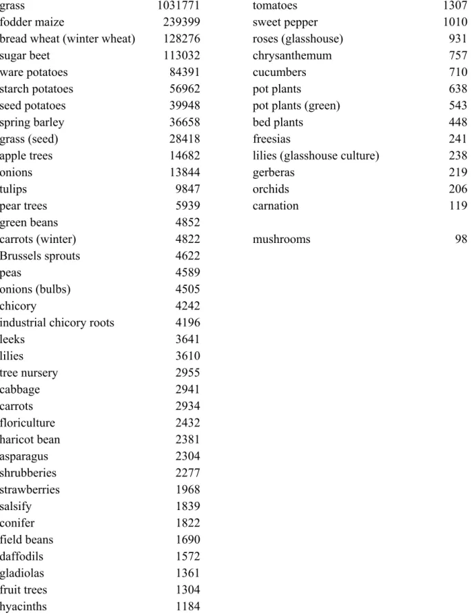
Table 2.1 Crops and total crop areas represented in the NMI
Crop (open culture) area (ha) Crop (covered cultures) area (ha)
grass 1031771 tomatoes 1307
fodder maize 239399 sweet pepper 1010
bread wheat (winter wheat) 128276 roses (glasshouse) 931
sugar beet 113032 chrysanthemum 757
ware potatoes 84391 cucumbers 710
starch potatoes 56962 pot plants 638
seed potatoes 39948 pot plants (green) 543
spring barley 36658 bed plants 448
grass (seed) 28418 freesias 241
apple trees 14682 lilies (glasshouse culture) 238
onions 13844 gerberas 219
tulips 9847 orchids 206
pear trees 5939 carnation 119
green beans 4852
carrots (winter) 4822 mushrooms 98
Brussels sprouts 4622
peas 4589
onions (bulbs) 4505
chicory 4242 industrial chicory roots 4196
leeks 3641 lilies 3610 tree nursery 2955 cabbage 2941 carrots 2934 floriculture 2432 haricot bean 2381 asparagus 2304 shrubberies 2277 strawberries 1968 salsify 1839 conifer 1822 field beans 1690 daffodils 1572 gladiolas 1361 fruit trees 1304 hyacinths 1184
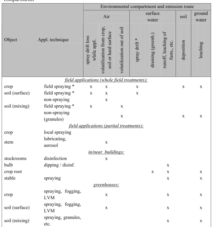
2.6 Application techniques
Data on application techniques were also obtained from LEI and CBS. The data are gathered along with the use data in the previous paragraph. The data were grouped to enable the
correct choice of the calculation method for the amount of pesticide emitted from the target area (Table 2.2). The way plant protection products are applied may affect the emission to environmental compartments and therewith the potential impact of the plant protection product.
Table 2.2: Application techniques, emission routes and receiving environmental compartments
Environmental compartment and emission route Air surface
water soil
ground water
Object Appl. technique
spray drift los
s while appl. volatilization from crop, soil or hard s urface volatilization out of soil spray drift * draining ( greenh.) runoff, leaching of
fusts,, etc. deposition leaching
field applications (whole field treatments):
crop field spraying * x x x x x
soil (surface) field spraying * x x x
non-spraying x
soil (mixing) field spraying * x x non-spraying
(granules) x x x
field applications (partial treatments):
crop local spraying
stem lubricating,
aerosol x
in/near buildings:
stockrooms disinfection x
bulb dipping / disinf. x
crop root x x x
stable spraying x x
greenhouses:
crop spraying, fogging,
LVM x x x
soil (surface) spraying, fogging,
LVM x x x
soil (mixing) spraying, granules,
etc. x x
*) Field spraying by a field sprayer in combination with drift reducing methods (see Drift section)
2.7 Crop interception
Data on interception of PPP by plants were taken from the interception tables used by CTB. These tables are liable to changes and, therefore, the NMI tables will need regular updates.
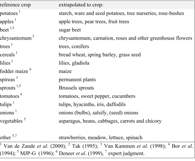
Interception depends on the relative coverage of the soil and therefore on the growth stage of the crop. Interception will therefore vary during the growing season. Growth curves, relating crop stage to week numbers, were established for all crops that are included in the NMI. Using these curves, interception factors were derived based on interception measurements. As interception measurements were not available for all crops extrapolations to other crops had to be made. Table 2.3 gives an overview of the extrapolations.
Table 2.3: Extrapolated interception factors for all crops in the NMI
reference crop extrapolated to crop:
potatoes 1 starch, ware and seed potatoes, tree nurseries, rose-bushes apples 1 apple trees, pear trees, fruit trees
beet 1,5 sugar beet
chrysantemum 2 chrysantemum, carnation, roses and other greenhouse flowers
trees 1 trees, conifers
cereals 1 bread wheat, spring barley, grass seed
lilies 1 lilies, gladiola
fodder maize 6 maize
spireas 3 permanent plants
sprouts 1,5 Brussels sprouts
tomatoes 4 tomatoes, sweet pepper, cucumbers tulips 1 tulips, hyacinths, iris, daffodils onions 1 onions (bulbs), salsify, (seed) onions
vegetables 5 asparagus, beans, cabbages, carrots and chicory
other 5,7 strawberries, meadow, lettuce, spinach 1 Van de Zande et al. (2000); 2 Tak (1995); 3 Van Kammen et al. (1998); 4 Bor et al. (1994); 5 MJP-G (1996); 6 Deneer et al. (1999), 7 expert judgment.
2.8 Drift
Drift data were constituted using four data sources:
• data on spraying equipment and spraying techniques, resulting from the surveys by Statistics Netherlands (see also paragraph 2.5);
• spray drift data for standard spraying techniques under standard conditions, derived from research by Porskamp et al. (2001);
• spray drift reduction data resulting from measures to reduce spray drift to surface water; • data on the degree of implementation of such measures in Dutch agriculture (Wingelaar
et al., 2001).
This information was used to construct drift tables for 1998 and 1999. By regulation (LOTV), Dutch farmers should apply drift reduction techniques when spraying plant protection products in the open field near open water. Minimum drift reductions percentages, resulting
from these techniques, are given in the regulation. These reduction percentages were included in the drift tables for 2000 and 2001.
2.9 Substance fate and ecotox data
For calculating environmental exposure a number of physico-chemical and fate data of plant protection products are necessary. The physico-chemical data include: molar mass, saturated vapour pressure and solubility in water. For acidic substances in addition the acid dissociation constant (pKa) is necessary. The fate data include: the constant for sorption on soil organic matter (Kom) (for acidic substances for both the molecular and the ionic species) and the transformation constant (DegT50) in soil under reference conditions. For metabolites essentially the same information is necessary and, in addition, the formation fraction, i.e. the molar fraction of the parent that is transformed into the metabolite. So far, mean values for the fate data were used in the calculations.
Most of the physico-chemical data were available from existing databases, available at RIVM1. If physico-chemical data were missing in these databases, data from the pesticide handbook (Tomlin, 2002) were taken to complete the dataset. For inorganic substances data on the saturated vapour pressure usually are not available; for these substances the saturated vapour pressure values were all set to zero. Volatilisation of these inorganic substances from plant and soil surfaces will not occur in practice. Also, most of the fate data were available from existing databases at RIVM. For acidic substances only an approximate value for the sorption constant of the anionic species was included in these databases; for these substances Kom-values for both the acidic molecule and the anion were derived from CTB files and included. If fate data were missing for individual substances then CTB files were searched to find the necessary data.
For non-uniquely defined substances, for example mineral oil, Kom-values and DegT50-values do not exist; it was decided to leave records empty for these substances. In the calculations for leaching, the median leaching fraction or leaching concentration of all substances was taken as input for further calculations. The median leaching concentration is considered a better estimate of leaching than a value calculated using average values for Kom and DegT50. The ecotox data include LC50, EC50, LD50 and NOEC values for algae, birds, daphnia, earthworms and fish. In general only data from first tier experiments are available.
Availability of ecotox data in RIVM databases was much less. Therefore, it was decided to use ecotox data for algae, daphnia and fish from the database of the Dutch Centre for Agriculture and the Environment (CLM). These data are kept updated with registration data by CLM. The data were supplemented with RIVM ecotox data on earthworms and birds. For data gaps, the filling procedure as developed by Luttik and Kalf (1998) was used. This procedure uses data from other substances to fill data gaps. Firstly, the substance is described in terms of: functional group (fungicide, herbicide, insecticide), chemical group (for example
1 These databases partly were established using pesticide registration data as part of the reviewing and evaluation process.
organo-P) and mode of action (for example choline-esterase inhibition). Then, using this hierarchical order, a subset of data is taken from the database and the geometrical mean of the data is calculated. This geometrical mean is used to fill the gap. If data on the lowest level are missing, then the next higher hierarchical level data are used and so on. If this procedure was not successful, an overall geometric mean of all data was calculated and used.
3 Emission Indicators
One of the features of the NMI is that it can calculate emissions of plant protection products to non-target areas and compartments. The following non-target areas and compartments are distinguished:
• air
• groundwater; • surface water;
• neighbouring nature areas.
This chapter describes the methods for calculating the emissions.
3.1 Air
Volatilisation to air is calculated for four routes: • Volatilisation during application;
• Volatilisation from plant leaves; • Volatilisation from the soil surface; • Volatilisation from the bulk soil.
Volatilisation during application was studied by Holterman (2000); his results are included in the NMI. For a typical spray application on arable fields 3% of the applied amount stays in the air for a longer period and can be transported to outside the treated area. A part of the spray-droplets is or becomes so small that they stay air-born and their residence in the air is prolonged. The fraction volatilised during spraying when using an axial sprayer, as for instance in fruit cultivation and tree nurseries, might be higher. Data to support this assumption are lacking.
The volatilisation from plant leaves is calculated using the regression equation (Smit et al., 1998; Smidt et al., 2000):
(
CVcrop)
1.661 log( )
Psatlog = + Eq.3-1
with:
CVcrop the cumulative volatilisation, (% of amount reaching the crop)
Psat the saturated vapour pressure of the substance, (mPa), Psat ≤ 11.8 mPa.
The regression equation is based on a relatively small number of experiments. Psat is dependent on the temperature and therefore the amount volatilised is dependent on the time and the place of application, which determine the temperature. If Psat ≥ 11.8 mPa the cumulative volatilisation is taken to be 100%; substances having such a high Psat are not likely to be sprayed on crops.
The total amount of substance volatilised from the crop is calculated according to: 100 , A f CV Ecropair crop I
⋅ ⋅
= Eq.3-2
with
Ecrop,air the total amount volatilised from the crop, (kg ha-1) A the nominal rate for a single application, (kg ha-1) fI fraction intercepted by the crop, (-)
100 factor to convert from % to fraction
Volatilisation from the soil surface is also calculated using a regression equation (Smit et al., 1997; Smidt et al., 2000):
(
gas)
soil FP
CV =71.9+11.6log Eq.3-3
with
CVsoil the cumulative volatilisation from the soil surface (% of amount reaching the soil) FPgas fraction in the gas phase, calculated from:
sl soil liquid gas gas gas K K K FP lg lg ρ ε ε ε + + = Eq.3-4 with
FPgas the fraction of substance in the gas phase, (-)
εgas the volumetric gas fraction, (volume gas per volume soil)
εliquid the volumetric liquid fraction, (volume soil solution per volume soil) ρsoil the soil dry bulk density, (kg m-3)
Klg the liquid to gas partitioning coefficient, (-) Ksl the soil to liquid partitioning coefficient, (m3 kg-1)
The volatilisation from the soil surface is dependent on the time of application (as this influences temperature) and the location (as this determines temperature and soil type and, therefore, FPgas). The total amount volatilised from the soil surface is:
100 , A f CV E soil V air soil ⋅ ⋅ = Eq.3-5 with
Esoil,air the total amount volatilised from soil, (kg ha-1) fV fraction volatilised from soil, (-)
The amount of substance volatilised from the bulk soil usually is negligible, except for soil fumigants. For the soil fumigants off-line calculations with the PEARL model have been performed and the results introduced in the NMI database.
The total volatilisation (emission to air) for each substance is the sum of the individual volatilisation routes.
3.2 Groundwater
The NMI calculates leaching to groundwater starting from the net soil deposition:
(
al d i v w)
N A f f f f f
S = ⋅ 1− − − − + Eq.3-6
with:
SN the net soil deposition, (kg ha-1)
fal fraction lost by volatilisation during application, (-, default 0.03 for spray applications)
fd fraction lost by spray drift to surroundings of the treated field, (-) fw fraction wash-off from the crop canopy, (-, default 0)
The nominal rate for a single application is obtained from the pesticide use table, which is based on pesticide use inventories by Statistics Netherlands (CBS) and the Agricultural Economics Research Institute (LEI) (see chapter 2.4). For a detailed description: see Smidt et
al. (2002). The fraction washed off from the canopy is unknown; information on this fraction
is lacking and the (default) value is taken to be zero.
The leaching process is relatively slow compared to other emission processes and, therefore, transformation processes have to be taken into account when calculating emissions due to leaching. Transformation results in dissipation of a plant protection product and only a fraction of the net soil deposition will leach to groundwater. Transformation however also results in metabolites or other degradation products. (In the remainder of the text the term metabolites includes also the other degradation products.) Some of the metabolites are considered relevant from the registration point of view and the leaching of these relevant metabolites is included in the NMI.
The leaching of a substance is highly dependent on environmental conditions and chemical properties of the substance. The use of a generic leaching fraction is therefore not possible. Instead, a leaching fraction is calculated for each substance separately (see section 3.2.1) and this leaching fraction is used to calculate the leaching amount. The leaching to the depth of approximately one metre below soil surface is calculated from:
N PEARL p gw F S E , = ⋅ Eq.3-7 N PEARL m p p m m gw f F S M M E , = ⋅ , ⋅ ⋅ Eq.3-8 with
Egw predicted amount leaching to groundwater (depth one metre), (kg ha-1)
FPEARL the leaching fraction obtained from the PEARL metamodel (see section 3.2.1), (-) SN the net soil load, (kg ha-1)
M molar mass, (g mol-1)
fp,m the molar fraction of a parent molecule converted to the metabolite2, (-) p, m parent resp. metabolite
The total amount leaching to groundwater at a depth of one metre is the sum of the amounts calculated for the parent and all relevant metabolites.
For multiple applications a four-step approach is followed: 1. determination of the net soil load for each single application;
2. determination of the total net load by summing the loads of the individual applications; 3. determination of the central application time;
4. calculation of the leaching as for a single application, with the total net load and the central application time as main input.
There is no correction for transformation of substances in between the applications. This is because transformation is already accounted for in the PEARL model; correction would lead to an overestimation of the transformation.
3.2.1 Metamodel of PEARL
The NMI uses a metamodel of the PEARL model (Tiktak et al., 2000; Leistra et al., 2001) to calculate leaching to groundwater. The metamodel interpolates (logarithmically) between results obtained for standard runs with the PEARL model, using the half-life and the sorption constant of the plant protection product. The standard runs consisted of runs with the standard Dutch scenario for variable half-life (1 - 200 d), variable sorption constant (0 - 200 dm3 kg-1) and variable application time (one for each month). A standard spray application of 1 kg ha-1 to the soil surface was assumed and volatilisation was switched off. As results the maximum average concentrations (mg m-3 or µg dm-3) in the upper metre of the groundwater or the fraction leached to groundwater are used. The metamodel is comparable with the method used in pesticide registration (Linders and Jager, 1998).
Spatial variation in leaching is approximated by accounting for differences in temperature and differences in soil organic matter content in the grid cells. Differences in temperature are
2The molar fraction here is the fraction of the metabolite compared to the parent (the plant protection product applied).
accounted for by calculating the local half-life for the plant protection product and using this local half-life in the interpolation procedure. The local half-life is calculated according to:
T l f DegT DegT50, = 50 Eq.3-9 with ⎟ ⎟ ⎠ ⎞ ⎜ ⎜ ⎝ ⎛ ⎟ ⎟ ⎠ ⎞ ⎜ ⎜ ⎝ ⎛ − ∆ − = SS gridcell T T T T R H f exp 1 1 Eq.3-10 and
DegT50,l the local half-life in the grid cell, (d)
DegT50 the nominal half-life of the substance as listed in the substance table, (d) fT factor denoting the influence of temperature, (-)
∆HT molar enthalpy of transformation, (J mol-1), (default value 54 kJ mol-1) R molar gas constant, (J mol-1 K-1), (value 8.3 J mol-1 K-1)
Tgridcell yearly average temperature of the grid cell, (K)
TSS yearly average temperature of reference scenario, (K), (value 282.21 K ≡ 9.21 ºC) Differences in soil organic matter are accounted for by calculating local sorption constants. The local sorption constant of a substance in this approach is calculated from the sorption constant in the substance table and the organic matter content in the top layer (plough layer) of the soil, which is dependent on the location:
om ref grid om K om om K * = ⋅ Eq.3-11 with
Kom* the local sorption constant, (dm3 kg-1)
Kom the sorption constant from the substance table, (dm3 kg-1)
omgrid the organic matter content in the plough layer of the grid cell, (%) omref the organic matter content in the plough layer of the reference, (%)
The organic matter content of the plough layer is chosen, because the majority of the transformation in general takes place in the plough layer of the soil; transformation in deeper layer is usually less. The local sorption constant is used in the interpolation process.
In case of slightly acidic substances, there is a further correction for the pH of the grid cell. Firstly, a combined sorption constant for the acidic molecule and its conjugated base is calculated:
(
)
(
)
a a pK gridcell pH base om pK gridcell pH acid om com om molarmass molarmass K molarmass molarmass K K − − ⋅ − + ⋅ ⋅ − + = , , , , , 10 1 1 10 1 Eq.3-12 withKom,com the combined sorption constant, (dm3 kg-1)
Kom,acid the sorption constant of the acidic molecule, (dm3 kg-1) Kom,base the sorption constant of the conjugated base, (dm3 kg-1) molarmass molar mass of the acidic molecule, (g mol-1)
pHgridcell the pH of the top soil of the grid cell, (-) pKa the dissociation constant of the substance, (-)
Secondly, the local sorption of the substance is then calculated from:
com om ref grid om K om om K * = ⋅ , Eq.3-13
and this local sorption constant is used to interpolate in the metamodel. The procedure described above is identical for metabolites.
The approach is an extension of the approach used in pesticide registration; this approach accounts for temporal and spatial variability in contrast to the registration procedure in the Netherlands3.
3.3 Surface water
The total loss of pesticides by spray drift may partially be deposited on watercourses and surface water. Other areas on which spray drift may be deposited are: agricultural area outside the treated field, nature area and built-up area. In the NMI three receiving areas are considered: the watercourses, the surface water and the nature area. The amounts entering the
3 Procedures to account for temporal and spatial variability in leaching in the pesticide registration procedure are under development and it is envisaged that these will be implemented soon.
The term surface water is used in two different senses in the Netherlands:
1. in pesticide registration, surface water is the water in watercourses that may be exposed to plant protection products;
2. in (overall) pesticide policy, surface water is defined as the body potentially holding water, i.e. the watercourse and its side-slopes.
When in pesticide policy reference is made to emissions to surface water, then the second definition is used; drift to watercourses contributes to these emissions. The two apprehensions have impact on the calculation routines in the NMI. To avoid confusion, in this report the term surface water will be used when referring to the first sense and the term watercourse for the second sense.
watercourse or the nature area are calculated using appropriate values for the drift factors (see chapter 2.7). The emission by drift to surface water is:
2 100 10 % 4 , , ⋅ ⋅ ⋅ ⋅ ⋅ = driftsw sw sw d sw W L A E Eq.3-14 with
Esw,d the emission to surface by the drift process, (kg ha-1)
%drift,sw the % drift as influenced by application technique and drift reducing measures (see chapter 2.7), (-)
Lsw the length of the surface water (per ha field), (m) Wsw the width of the surface water, (m)
The factors 104 and 100 in the denominator are to convert from kg ha-1 to kg m-2 and from % to fraction. The factor 2 in the denominator is to account for the wind direction: it is assumed that only surface water downwind from the treated area is exposed.
Another route of plant protection products to surface water is drainage. Water infiltrating in the soil may drain to surface water, sometimes via artificial drains. The emission of plant protection products to surface water via this route is calculated in a two-stage procedure. Firstly, in an off-line procedure, the amounts of water flowing to the groundwater and to surface water via artificial and natural drainage systems were calculated, using the GeoPEARL package (Tiktak et al., 2004). The results are stored in the NMI database as fractions of the total net amount of water passing the depth of 1 m. Secondly, the emission to surface water as result of lateral drainage is calculated according to:
dr PEARL N ld sw S F F E , = ⋅ ⋅ Eq.3-15 with
Esw,ld the emission to surface water by the lateral drainage process, (kg ha-1) Fdr the fraction of the water draining to surface water, (-)
The total emission to surface water is the sum of the amounts from the drift process and the lateral drainage process:
ld sw d sw sw E E E = , + , Eq.3-16
3.4 Neighbouring nature areas
Drift to neighbouring nature areas is calculated analogously to drift to surface water. Two situations may occur:
1. the nature area is immediately adjacent to the treated field; 2. the nature area is situated on the other side of the water course.
In situation 1, the total amount of spray drift is deposited on the nature area. In the calculation all measures that reduce drift are accounted for. In situation 2, the total amount of drift is diminished by the amount deposited in between the field and the edge of the nature area. Whether or not nature area and ditches occur is derived from the land use database. The amounts are calculated according to:
2 100 % , , ⋅ ⋅ ⋅ = driftN N d N L A E Eq.3-17 with
EN,d the amount emitted to nature areas via drift, (kg ha-1)
%drift,N the % drift to nature; appropriate % should be chosen for the situations with and without surface water between the treated field and the nature area, also accounting for drift reduction (see also chapter 2.7), (-)
LN the length of the nature area per ha treated field, (m)
The factor 100 in the denominator is to convert from % to fraction and the factor 2 is to account for the wind direction; it is assumed that only downwind areas are exposed to drift.
4 Effect indicators
4.1 Soil
The general principle of comparing an exposure concentration with ecotoxicological data for organisms or the ecosystem is followed for the soil environment. Soil here is defined as the top layer of the treated field. For the thickness of this top layer the following default values apply:
• 0.05 m for spray applications when assessing acute and chronic risk;
• 0.05 m for injection applications, treated seeds, bulbs and tubers when assessing acute and chronic risk;
• 0.2 m for applications incorporated in soil when assessing acute and chronic risk.
The exposure concentration is calculated from the net soil deposition, soil characteristics obtained from the soil map of the Netherlands and, when relevant, the transformation rate of the substance.
4.1.1 Soil exposure concentration, single application
Ecotoxicological data for soil organisms have the dimension [M M-1] and therefore the exposure concentration also has the same dimension. Input to the calculation of the exposure concentration is the net soil deposition. The net soil deposition is calculated from the nominal application rate and several loss terms (see also Eq.3-4):
(
al d i v w)
N A f f f f f
S = ⋅ 1− − − − + Eq.4-1
with
SN the net soil deposition, (kg ha-1)
A (nominal) application rate (one application), (kg ha-1) Fal fraction lost by volatilisation during application, (-)
Fd fraction lost by drift to surroundings of the treated field (surface water and nature), (-) Fi fraction intercepted by the crop, (-)
Fv fraction volatilised from the soil, (-)
Fw fraction washed off from the crop, reaching the soil, (-)
All loss fractions play a role when a crop protection product is sprayed over the crop. When another application technique is used, for instance injection or incorporation, some of the loss fractions may be absent.
The nominal application rate and the loss fractions are derived from procedures as described in chapter 2. The fractions lost by volatilisation during application and drift depend on application technique and reduction measures as described elsewhere (Smidt et al., 2000; Smidt et al., 2002; chapter 2). The fraction intercepted is dependent on the crop type and the growth stage of the crop, which in turn is dependent on the time (moment in the growth
cycle). The fraction volatilised from the soil is dependent on physico-chemical properties of the crop protection product, soil characteristics, soil conditions and climate conditions (see chapter 3.1).
We may now convert the amount reaching the soil into a soil content to make an ecotoxicological assessment possible:
soil soil N d S G ρ ⋅ ⋅ = 4 10 Eq.4-2 with
G the content of the substance in the soil, (kg kg-1) dsoil the depth (thickness) of the soil layer, (m) ρsoil the dry bulk density of the soil, (kg m-3)
The dry bulk density is dependent on the soil type and therefore obtained from the soil map. The factor 104 is used to convert from kg ha-1 (the unit for application rates that is generally used) to kg m-2. Depending on the type of risk assessment – acute or chronic – and the application type – spraying, injection or incorporation - the depth over which the substance distributes is 5 to 20 cm. Usually, ecotoxicological data for soil organisms or soil functions are expressed as mg active ingredient per kg dry soil (mg kg-1). Conversion to these units invokes a factor of 106 in the numerator of the equation. The soil dry bulk density varies with soil type and ranges from approximately 1000 to 1700 kg m-3. If not available as a map attribute, the dry bulk density may be calculated from soil texture and the organic matter content of the soil, using a pedotransfer function (Wösten et al., 1994).
4.1.2 Soil exposure concentration, multiple applications
If there is more than one application, the residues in soil may build up. A new application adds to the remains of the former application(s):
G X
XTA = R + Eq.4-3
with:
XTA the content in soil immediately after the last application, (kg kg-1)
XR the content in soil immediately before the last application, (kg kg-1), the remains of former applications
The remains are calculated according to a (pseudo) first-order equation: t k f TA t T e X X = ⋅ − ⋅⋅ Eq.4-4 with:
Xt the content in soil at time t, (kg kg-1)
k first order rate coefficient for transformation in soil, (d-1) t time (= time elapsed after last application), (d)
fT factor for the influence of temperature, (-).
X can be expressed as a content, but also as an absolute amount. In a first-order rate equation, the transformation rate is independent of the concentration. As the soil bulk density is assumed constant for the top layer, the ratio between the amount in the soil and the soil content is constant. Usually the half-life (DegT50) of a substance is stored in databases. In the NMI half-lives for substances are stored in a substance table. The half-lives refer to standard conditions, i.e. 20 °C, top soil at pF = 2. The rate coefficient is calculated from the half-life according to:
50 ln(2)
DegT
k = Eq.4-5
In most models, used for registration purposes, the transformation is dependent on soil temperature, soil moisture and depth in the soil profile. For the soil compartment in the NMI, depth is not relevant because only the top layer of the soil is considered. In modern agriculture crops are irrigated when necessary; therefore the influence of soil moisture can be neglected as well. This leaves temperature as the only influencing factor. The influence of temperature is given by the Arrhenius equation:
⎟ ⎟ ⎠ ⎞ ⎜ ⎜ ⎝ ⎛ ⎟⎟ ⎠ ⎞ ⎜⎜ ⎝ ⎛ − ∆ − = r T T T T R H f exp 1 1 Eq.4-6 with
fT factor denoting the influence of temperature, (-)
∆HT molar enthalpy of transformation, (J mol-1), (default value 54 kJ mol-1) R molar gas constant, (J mol-1 K-1), (value 8.3 J mol-1 K-1)
T temperature, (K)
Tr reference temperature, (K), (value 293 K ≡ 20 ºC, because of the requirements imposed on the substance database).
For acute assessments the peak content is used to compare with the ecotoxicological data for earthworms. Now the calculation of the peak content is not straightforward. The net deposition is not constant as one or several factors, for instance interception, may vary in
time. Also temperature varies in time, causing the transformation to increase (raising temperature) or decrease (falling temperature). A numerical model has been built to calculate the peak content (amount). For all repeated applications, it is assumed that the interval period is fixed at 7 days, i.e. there is a time lapse of 7 days between two applications. The result of the calculations, the soil content versus time, has the form of a saw-tooth line. The maximum content is taken for comparison with ecotoxicological data (see section 4.1.3).
4.1.3 Potential acute effects in soil
Toxicity data for soil organisms usually are expressed in mg kg-1. The substance database contains LC50 data for earthworms (LC50,earthworm) in mg kg-1. These data are derived from standard experiments with earthworms, for which a standard soil type containing 10% organic matter and 25% clay is used. Before Environmental Indicator Units (EIU) can be calculated, two conversions are necessary: the peak content has to be expressed in mg kg-1 (Eq.4-7) and the LC50,earthworm has to be corrected for differences in the organic matter content of the soil in the grid cell and the organic matter content of the earthworm toxicity test soil (Eq.4-8).
TA
soil X
PIEC =106⋅ Eq.4-7
with
PIECsoil predicted initial environmental concentration in soil, (mg kg-1) 106 conversion factor from kg kg-1 to mg kg-1.
ref gridcell earthworm a soil OM OM LC ECC % % , 50 , = ⋅ Eq.4-8 with
ECCsoil,a environmental concern concentration for the soil, (mg kg-1)
LC50,earthworm 50% lethal concentration for earthworms under reference conditions, (mg kg-1) OM%gridcell organic matter of the grid cell soil, (percentage)
OM%ref organic matter of the reference, (percentage) (default value 10 %) The number of Environmental Indicator Units is now calculated from:
acute soil soil a soil ECC PIEC EIU , , 001 . 0 ⋅ = Eq.4-9 with:
4.2 Groundwater
The general principle of comparing an exposure concentration with ecotoxicological data for organisms or the ecosystem is not followed for the groundwater environment; instead the threshold value for pesticides in drinking water is used. Groundwater here is defined as the water present in the top meter of the saturated zone beneath the treated field. In general there is some time lapse in between the application of the pesticide and the occurrence of the substance in groundwater. Therefore, the groundwater indicator is regarded as a chronic indicator. As described in section 3.1, the NMI uses a metamodel of the PEARL model for these calculations. Instead of leached amounts the concentration of the plant protection product or its relevant metabolites in the uppermost groundwater is used.
4.2.1 Groundwater exposure concentration
The drinking water threshold level has the dimension of concentration [M L-3] and therefore the exposure concentration should also have the same dimension. Therefore, an analogous procedure to the calculation of leaching emission (see sections 3.2 and 3.2.1) is used. Instead of a fraction leached to groundwater, now the resulting concentration in the groundwater is used. In the procedure the fraction leached (FPEARL) is replaced by the concentration (CPEARL):
T N PEARL p gw C S PEC , = ⋅ , Eq.4-10 T N PEARL m p p m m gw f C S M M PEC , = ⋅ , ⋅ ⋅ , Eq.4-11 with
PECgw predicted environmental concentration in groundwater, (mg m-3)
CPEARL the concentration obtained via interpolation in the PEARL metamodel, (mg m-3) SN,T the net soil load, (kg ha-1)
M molar mass, (g mol-1)
fp,m the molar fraction of a parent molecule converted to the metabolite, (-) p, m parent resp. metabolite
If there is more than one metabolite, the calculation is repeated for each metabolite. The conversion fractions (fp,m) always relate the metabolite to the parent, also when the conversion is via other metabolites. Note that this procedure is different from the procedure in the PEARL model; there second generation metabolites are related to the first generation metabolites, and so on.
4.2.2 Potential effects in groundwater
Environmental Indicator Units are derived from the comparison of the groundwater exposure concentration, PECgw, with the threshold level for substances in drinking water:
TLD PEC
EIUgw = gw Eq.4-12
with
EIUgw environmental indicator units for groundwater, (-)
TLD threshold limit for substance in drinking water, (mg m-3, default 0.1)
This calculation is repeated for each of the relevant metabolites and the EIUgw are summed to give the final potential effect of the application.
4.3 Surface water
The general principle of comparing an exposure concentration with ecotoxicological data for organisms or the ecosystem is followed for the surface water environment. Surface water in the current version of the NMI is assumed to be a water body with a surface width of 1 m, a depth of 0.3 m and slopes of 45 degrees. So per m2 water surface the water content of the surface water body is 0.21 m3 (210 dm3). The length of the water bodies varies from grid cell to grid cell; the length is taken into account in the calculation of EIUs.
The exposure concentration is calculated from the drift deposition, which in turn is dependent on application technique, crops factors and emission reduction measures. EIUs are calculated for algae, daphnids, fish or the aquatic system as a whole.
4.3.1 Surface water exposure concentration, single application
Ecotoxicological data for surface water organisms have the dimension [M L-3] and therefore the exposure concentration should be expressed in the same dimension. Input to the calculation of the exposure concentration is the net surface water deposition. This surface water deposition is calculated from the nominal application rate and a drift factor:
A f
Ssw = d,sw⋅ Eq.4-13
with:
Ssw the net surface water deposition, (kg ha-1 (surface water)) fd,sw fraction drift to surface water, (-)
A (nominal) application rate (one application), (kg ha-1)
The drift factor indicates the deposition of spray drift averaged over the width of the water body. Note that fd,sw is different from fd mentioned in Eq.4-1. The initial concentration in the surface water can now be calculated from the dimensions of the water body and the net surface water deposition:
⎟⎟ ⎠ ⎞ ⎜⎜ ⎝ ⎛ − ⋅ ⋅ = α tan 10 2 sw sw sw sw sw d d w S PIEC Eq.4-14 with:
PIECsw the initial concentration in surface water immediately after application, (mg dm-3) 10 conversion factor from kg ha-1 to g m-2
wsw width of the surface water (wet surface) dsw depth of the surface water
α acute angle of the slope of the ditch with the soil surface
4.3.2 Surface water exposure concentration, multiple applications
If there is more than one application, the residues in surface water may build up. A new application adds to the remains of the former application(s):
sw r sw ta sw S S S , = , + Eq. 4-15 with:
Ssw.ta the amount in surface water immediately after the last application, (kg ha-1)
Ssw,r the amount in surface water immediately before the last application, (kg ha-1), the remains of former applications
The remains are calculated according to a first-order equation: t k f ta sw t sw sw T sw e S S = ⋅ − , ⋅ ⋅ , , Eq. 4-16 with:
Ssw,t the amount in surface water at time t (= time elapsed after last application), (kg ha-1) ksw first order rate coefficient for dissipation in surface water, (d-1)
t time, (d)
fsw,T factor for the influence of the temperature of the surface water body, (-).
Usually the half-life (DegT50,sw) or the dissipation half-life (DT50,sw) of a substance is stored in databases. In the NMI lives for substances are stored in a substance table. The lives refer to standard conditions, i.e. 20 °C. The rate coefficient is calculated from the half-life according to one of the following equations:
sw sw DegT k , 50 ) 2 ln( = Eq.4-17a sw sw DT k , 50 ) 2 ln( = Eq.4-17b
In most models, used for registration purposes, the transformation is dependent on temperature. The influence of temperature is given by the Arrhenius equation (see also Eq.4-6): ⎟ ⎟ ⎠ ⎞ ⎜ ⎜ ⎝ ⎛ ⎟⎟ ⎠ ⎞ ⎜⎜ ⎝ ⎛ − ∆ − = r T T sw T T R H f , exp 1 1 Eq.4-18 with
fsw,T factor denoting the influence of temperature, (-)
∆HT molar enthalpy of transformation, (J mol-1), (default value 54 kJ mol-1) R molar gas constant, (J mol-1 K-1), (value 8.3 J mol-1 K-1)
T temperature, (K)
Tr reference temperature, (K), (value 293 K ≡ 20 ºC, because of the requirements imposed on the substance database).
For acute assessments a peak concentration is used to compare with the ecotoxicological data. Now the calculation of the peak concentration is not straightforward. The net deposition is not constant as one or several factors influencing drift may vary in time. Also temperature may change, causing the dissipation rate to increase (raising temperature) or decrease (falling temperature). A numerical model has been built to calculate the peak concentration. In the current version of the NMI the interval period is fixed at 7 days, i.e. it is assumed that there is a time lapse of 7 days between two applications.
The initial concentration in the surface water can now be calculated from the dimensions of the water body and the net surface water deposition (see also Eq.4-14):
⎟⎟ ⎠ ⎞ ⎜⎜ ⎝ ⎛ − ⋅ ⋅ = α tan 10 2 , SW sw sw ta sw sw d d w S PIEC Eq.4-19
4.3.3 Potential acute effects in surface water
The calculations in par. 4.2.1 and 4.2.2 give results for surface waters receiving a drift deposition, expressed as an amount per unit area surface water. In general only surface water leeward to the treated field will receive spray drift. The standard spray drift factors (as laid down in the drift table) are derived from field experiments on spray drift in which the wind direction was perpendicular to the surface water, with a tolerance of 30 degrees in either direction (Van de Zande et al., 2000) and the surface water leeward to the treated field. Surface water in the windward direction does not receive spray drift. When in practice the wind has a smaller angle with the surface water, the spray drift deposition may be overestimated.
A second factor, which is important in the calculation of the EIUs, is the length of the surface water body along the treated field. In pesticide registration in the Netherlands the length of the water body determines the number of applications that are considered in the calculation of the peak concentration. As the (fixed) length of the ditch is 320 m and the rate of the water flow is 10 m per day (in spring), a limited number of applications – depending on the application interval - is considered. The NMI disregards this limitation and considers all applications. Still, the length plays an important role as it is a measure of the total volume of water exposed to the substance. In the NMI calculations the length is incorporated relatively to the length of the surface water in a reference situation.
The EIUs for surface water are now calculated according to:
a sw sw DL W a sw ECC PIEC f f EIU , , * 01 . 0 ⋅ ⋅ = Eq. 4-20 with ref s sw gridcell s sw DL R R f , , , , = Eq. 4-21 and
EIUsw,a Environmental Indicator Units for surface water, acute, (-) fW factor accounting for wind direction, (-, default 0.5)
fDL factor accounting for ditch length, depending on map information, (-)
ECCsw,a environmental concern concentration for surface water, acute, (mg dm -3)
Rsw,s,gridcell surface water to soil ratio in the grid cell, (-)
Rsw,s,ref surface water to soil ratio in the reference situation, (-)
In surface water four separate indicators are distinguished when considering acute effects: 1 indicator for algae, ECCsw,a is then equal to the EC50 for algae (EC50,algae);
2 indicator for daphnids, ECCsw,a is then equal to the LC50 for daphnids (LC50,daphnids); 3 indicator for fish, ECCsw,a is then equal to the LC50 for fish (LC50,fish);
4 indicator for the aquatic ecosystem, ECCsw,a is then equal to the lowest of the three EC50 or LC50 values mentioned above.
4.4 Terrestrial organisms
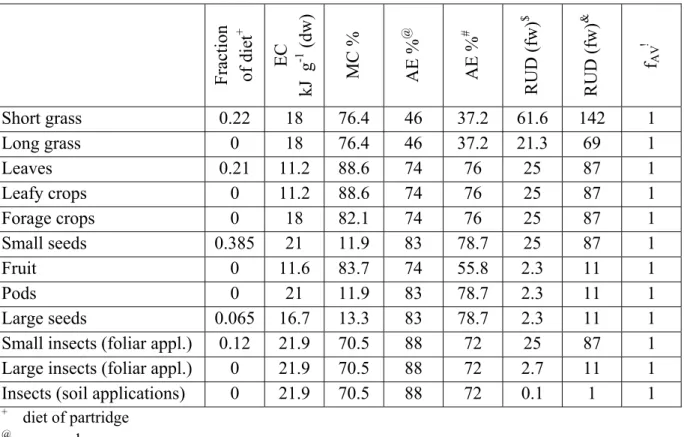
For the environmental indicator the partridge (body weight 370 g) is chosen as standard species, because birds are generally more sensitive than mammals and partridges are known to forage in field margins. It is assumed that the diet consists of 22% short grass, 21% leaves, 38.5% small seeds, 6.5% cereals and 12% small insects. Furthermore it is calculated with fresh weight data for food.
For the moment only potential impact of sprayed PPP are included in the NMI; potential impacts of seed dressings, injected or incorporated and granular applications will be added later.
4.4.1 Dietary exposure of birds and mammals by sprayed pesticides
The exposure of birds and mammals feeding on treated fields is calculated on the basis of the food consumption of the animals and the applied amount of plant protection product. As most toxicological experiments are performed using the nominal dosage, this dosage is used in the calculation. The daily chemical intake (DCI) for birds and mammals can be calculated with:
TWA AV f f A 1000 RUD 100 AE 100 MC 1 FE DEE DCI ⋅ ⋅ ⋅ ⋅ ⎟⎟ ⎠ ⎞ ⎜⎜ ⎝ ⎛ ⋅ ⎟ ⎠ ⎞ ⎜ ⎝ ⎛ − ⋅ = Eq.4-22 with:
DCI daily chemical intake, (mg d-1) DEE daily energy expenditure, (kJ d-1) FE food energy, (kJ per dry gram food) MC moisture content of the food, (%)
AE assimilation efficiency, dependent on the species, (%)
RUD residue unit dose (mg per kg fresh weight food per unit dose of 1 kg a.s. per hectare) A dosage, (nominal) application rate, (kg ha-1)
fAV avoidance factor (1= no avoidance, 0 = complete avoidance)
fTWA time weighted average fraction (default is no degradation for acute exposure and 0.53 for long term exposure (DT50 of 10 days))
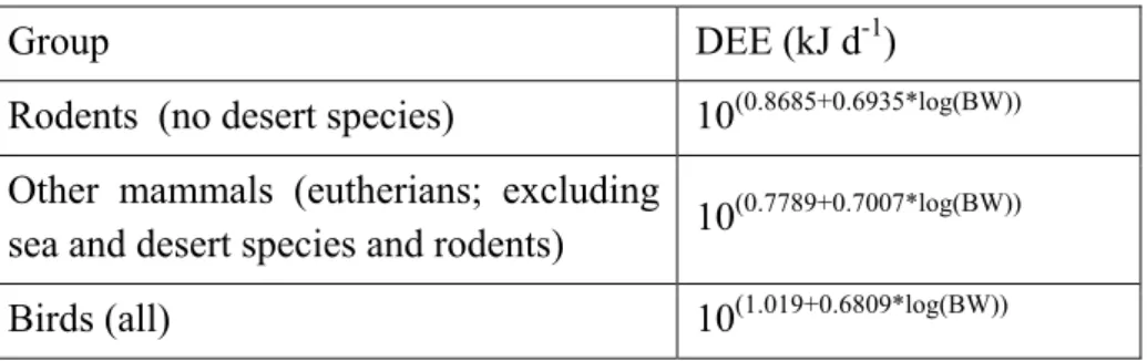
The DEE is different for birds and mammals and for the latter a distinction is made between rodents (no desert species) and other mammals (not including sea and desert species) (see Table 4.1). It is not necessary to differentiate between passerines and non-passerines, because the difference between the two groups is negligible.
Table 4.1 Daily energy expenditure (DEE) for different groups of birds and mammals (calculated with data provided by Nagy, 1987)
Group DEE (kJ d-1)
Rodents (no desert species) 10(0.8685+0.6935*log(BW)) Other mammals (eutherians; excluding
sea and desert species and rodents) 10
(0.7789+0.7007*log(BW))
Birds (all) 10(1.019+0.6809*log(BW)) Note: BW (body weight) in grams
Table 4.2 presents average RUD values for several types of food (after Luttik et al., 2001). The RUD for long-term exposure assessments are based on the 50th percentile of residue data and for short term exposure assessments on the 90th percentile of these data (realistic worst case assumption).
Table 4.2 Residue unit dose (RUD) values (mg kg-1 fresh weight food) for an application rate of 1 kg ha-1 (after Luttik et al., 2001).
Food type Food code
RUD for medium and long term exposure
(= 50th percentile)
RUD for acute / short term exposure (= 90th percentile) Short grass F1 61.6 142 Long grass F2 21.3 69 Leaves F3 25 87 Leafy crops F4 25 87 Forage crops F5 25 87 Small seeds F6 25 87 Fruit F7 2.3 11 Pods F8 2.3 11 Large seeds F9 2.3 11
Small insects (foliar appl.) F10 25 87 Large insects (foliar appl.) F11 2.7 11 Insects (soil applications) F12 0.1 1
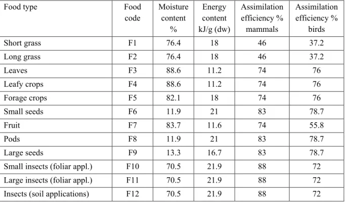
Table 4.3 lists the moisture content, the energy content and the assimilation efficiency for birds as well as for mammals for the same types of food.
Table 4.3 Moisture content, energy content, assimilation efficiency for different types of food for birds and mammals.
Food type Food
code Moisture content % Energy content kJ/g (dw) Assimilation efficiency % mammals Assimilation efficiency % birds Short grass F1 76.4 18 46 37.2 Long grass F2 76.4 18 46 37.2 Leaves F3 88.6 11.2 74 76 Leafy crops F4 88.6 11.2 74 76 Forage crops F5 82.1 18 74 76 Small seeds F6 11.9 21 83 78.7 Fruit F7 83.7 11.6 74 55.8 Pods F8 11.9 21 83 78.7 Large seeds F9 13.3 16.7 83 78.7
Small insects (foliar appl.) F10 70.5 21.9 88 72 Large insects (foliar appl.) F11 70.5 21.9 88 72 Insects (soil applications) F12 70.5 21.9 88 72