"Modular Forms, a Computational Approach"

(1)

Modular Forms:

A Computational Approach

William A. Stein

(with an appendix by Paul E. Gunnells)

Department of Mathematics, University of Washington

E-mail address: wstein@math.washington.edu

Department of Mathematics and Statistics, University of Massachusetts

(2)

Key words and phrases. abelian varieties, cohomology of arithmetic

groups, computation, elliptic curves, Hecke operators, modular curves, modular forms, modular symbols, Manin symbols, number theory

Abstract. This is a textbook about algorithms for computing with modular forms. It is nontraditional in that the primary focus is not on underlying theory; instead, it answers the question “how do you

(3)

v

(4)

(5)

Preface

This is a graduate-level textbook about algorithms for computing with mod-ular forms. It is nontraditional in that the primary focus is not on underly-ing theory; instead, it answers the question “how do you use a computer to

explicitly compute spaces of modular forms?”

This book emerged from notes for a course the author taught at Harvard University in 2004, a course at UC San Diego in 2005, and a course at the University of Washington in 2006.

The author has spent years trying to find good practical ways to compute with classical modular forms for congruence subgroups of SL2(Z) and has

implemented most of these algorithms several times, first in C++ [Ste99b], then in MAGMA [BCP97], and as part of the free open source computer algebra system SAGE (see [Ste06]). Much of this work has involved turning formulas and constructions buried in obscure research papers into precise computational recipes then testing these and eliminating inaccuracies.

The author is aware of no other textbooks on computing with modular forms, the closest work being Cremona’s book [Cre97a], which is about computing with elliptic curves, and Cohen’s book [Coh93] about algebraic number theory.

In this book we focus on how to compute in practice the spaces Mk(N, ε)

of modular forms, where k _{≥ 2 is an integer and ε is a Dirichlet character} of modulus N (the appendix treats modular forms for higher rank groups). We spend the most effort explaining the general algorithms that appear so far to be the best (in practice!) for such computations. We will not dis-cuss in any detail computing with quaternion algebras, half-integral weight forms, weight 1 forms, forms for noncongruence subgroups or groups other

(10)

than GL2, Hilbert and Siegel modular forms, trace formulas, p-adic modular

forms, and modular abelian varieties, all of which are topics for additional books. We also rarely analyze the complexity of the algorithms, but instead settle for occasional remarks about their practical efficiency.

For most of this book we assume the reader has some prior exposure to modular forms (e.g., [DS05]), though we recall many of the basic defini-tions. We cite standard books for proofs of the fundamental results about modular forms that we will use. The reader should also be familiar with basic algebraic number theory, linear algebra, complex analysis (at the level of [Ahl78]), and algorithms (e.g., know what an algorithm is and what big oh notation means). In some of the examples and applications we assume that the reader knows about elliptic curves at the level of [Sil92].

Chapter 1 is foundational for the rest of this book. It introduces congru-ence subgroups of SL2(Z) and modular forms as functions on the complex

upper half plane. We discuss q-expansions, which provide an important computational handle on modular forms. We also study an algorithm for computing with congruence subgroups. The chapter ends with a list of ap-plications of modular forms throughout mathematics.

In Chapter 2 we discuss level 1 modular forms in much more detail. In particular, we introduce Eisenstein series and the cusp form ∆ and describe their q-expansions and basic properties. Then we prove a structure theorem for level 1 modular forms and use it to deduce dimension formulas and give an algorithm for explicitly computing a basis. We next introduce Hecke operators on level 1 modular forms, prove several results about them, and deduce multiplicativity of the Ramanujan τ function as an application. We also discuss explicit computation of Hecke operators. In Section 2.6 we make some brief remarks on recent work on asymptotically fast computation of values of τ . Finally, we describe computation of constant terms of Eisenstein series using an analytic algorithm. We generalize many of the constructions in this chapter to higher level in subsequent chapters.

In Chapter 3 we turn to modular forms of higher level but restrict for simplicity to weight 2 since much is clearer in this case. (We remove the weight restriction later in Chapter 8.) We describe a geometric way of view-ing cuspidal modular forms as differentials on modular curves, which leads to modular symbols, which are an explicit way to present a certain homol-ogy group. This chapter closes with methods for explicitly computing cusp forms of weight 2 using modular symbols, which we generalize in Chapter 9. In Chapter 4 we introduce Dirichlet characters, which are important both in explicit construction of Eisenstein series (in Chapter 5) and in de-composing spaces of modular forms as direct sums of simpler spaces. The

(11)

Preface xiii

main focus of this chapter is a detailed study of how to explicitly represent and compute with Dirichlet characters.

Chapter 5 is about how to explicitly construct the Eisenstein subspace of modular forms. First we define generalized Bernoulli numbers attached to a Dirichlet character and an integer then explain a new analytic algorithm for computing them (which generalizes the algorithm in Chapter 2). Finally we give without proof an explicit description of a basis of Eisenstein series, explain how to compute it, and give some examples.

Chapter 6 records a wide range of dimension formulas for spaces of modular forms, along with a few remarks about where they come from and how to compute them.

Chapter 7 is about linear algebra over exact fields, mainly the rational numbers. This chapter can be read independently of the others and does not require any background in modular forms. Nonetheless, this chapter occu-pies a central position in this book, because the algorithms in this chapter are of crucial importance to any actual implementation of algorithms for computing with modular forms.

Chapter 8 is the most important chapter in this book; it generalizes Chapter 3 to higher weight and general level. The modular symbols for-mulation described here is central to general algorithms for computing with modular forms.

Chapter 9 applies the algorithms from Chapter 8 to the problem of computing with modular forms. First we discuss decomposing spaces of modular forms using Dirichlet characters, and then explain how to compute a basis of Hecke eigenforms for each subspace using several approaches. We also discuss congruences between modular forms and bounds needed to provably generate the Hecke algebra.

Chapter 10 is about computing analytic invariants of modular forms. It discusses tricks for speeding convergence of certain infinite series and sketches how to compute every elliptic curve over Q with given conductor.

Chapter 11 contains detailed solutions to most of the exercises in this book. (Many of these were written by students in a course taught at the University of Washington.)

Appendix A deals with computational techniques for working with gen-eralizations of modular forms to more general groups than SL2(Z), such as

SLn(Z) for n ≥ 3. Some of this material requires more prerequisites than

the rest of the book. Nonetheless, seeing a natural generalization of the material in the rest of this book helps to clarify the key ideas. The topics in the appendix are directly related to the main themes of this book: modular

(12)

symbols, Manin symbols, cohomology of subgroups of SL2(Z) with various

coefficients, explicit computation of modular forms, etc.

Software. We use SAGE, Software for Algebra and Geometry Experimen-tation (see [Ste06]), to illustrate how to do many of the examples. SAGE is completely free and packages together a wide range of open source math-ematics software for doing much more than just computing with modular forms. SAGE can be downloaded and run on your computer or can be used via a web browser over the Internet. The reader is encouraged to experi-ment with many of the objects in this book using SAGE. We do not describe the basics of using SAGE in this book; the reader should read the SAGE tutorial (and other documentation) available at the SAGE website [Ste06]. All examples in this book have been automatically tested and should work exactly as indicated in SAGE version at least 1.5.

Acknowledgements. David Joyner and Gabor Wiese carefully read the book and provided a huge number of helpful comments.

John Cremona and Kevin Buzzard both made many helpful remarks that were important in the development of the algorithms in this book. Much of the mathematics (and some of the writing) in Chapter 10 is joint work with Helena Verrill.

Noam Elkies made remarks about Chapters 1 and 2. S´andor Kov´acs provided interesting comments on Chapter 1. Allan Steel provided helpful feedback on Chapter 7. Jordi Quer made useful remarks about Chapter 4 and Chapter 6.

The students in the courses that I taught on this material at Harvard, San Diego, and Washington provided substantial feedback: in particular, Abhinav Kumar made numerous observations about computing widths of cusps (see Section 1.4.1) and Thomas James Barnet-Lamb made helpful re-marks about how to represent Dirichlet characters. James Merryfield made helpful remarks about complex analytic issues and about convergence in Stir-ling’s formula. Robert Bradshaw, Andrew Crites (who wrote Exercise 7.5), Michael Goff, Dustin Moody, and Koopa Koo wrote most of the solutions included in Chapter 11 and found numerous typos throughout the book. Dustin Moody also carefully read through the book and provided feedback. H. Stark suggested using Stirling’s formula in Section 2.7.1, and Mark Watkins and Lynn Walling made comments on Chapter 3.

(13)

Preface xv

Parts of Chapter 1 follow Serre’s beautiful introduction to modular forms [Ser73, Ch. VII] closely, though we adjust the notation, definitions, and order of presentation to be consistent with the rest of this book.

I would like to acknowledge the partial support of NSF Grant DMS 05-55776. Gunnells was supported in part by NSF Grants DMS 02-45580 and DMS 04-01525.

Notation and Conventions. We denote canonical isomorphisms by ∼= and noncanonical isomorphisms by≈. If V is a vector space and s denotes some sort of construction involving V , we let Vs denote the corresponding

subspace and Vs the quotient space. E.g., if ι is an involution of V , then V+is Ker(ι− 1) and V+= V /Im(ι− 1). If A is a finite abelian group, then

Ator denotes the torsion subgroup and A/tor denotes the quotient A/Ator.

We denote right group actions using exponential notation. Everywhere in this book, N is a positive integer and k is an integer.

If N is an integer, a divisor t of N is a positive integer such that N/t is an integer.

(14)

(15)

Chapter 1

Modular Forms

This chapter introduces modular forms and congruence subgroups, which are central objects in this book. We first introduce the upper half plane and the group SL2(Z) then recall some definitions from complex analysis. Next

we define modular forms of level 1 followed by modular forms of general level. In Section 1.4 we discuss congruence subgroups and explain a simple way to compute generators for them and determine element membership. Section 1.5 lists applications of modular forms.

We assume familiarity with basic number theory, group theory, and com-plex analysis. For a deeper understanding of modular forms, the reader is urged to consult the standard books in the field, e.g., [Lan95, Ser73, DI95, Miy89, Shi94, Kob84]. See also [DS05], which is an excellent first intro-duction to the theoretical foundations of modular forms.

1.1. Basic Definitions The group SL2(R) = ½µ a b c d ¶ : ad− bc = 1 and a, b, c, d ∈ R ¾

acts on the complex upper half plane

h=_{{z ∈ C : Im(z) > 0}}

by linear fractional transformations, as follows. If γ =¡a b c d

¢

∈ SL2(R), then

for any z∈ h we let

(1.1.1) γ(z) = az + b

cz + d ∈ h.

(16)

Since the determinant of γ is 1, we have µ d dzγ ¶ (z) = 1 (cz + d)2.

Definition 1.1 (Modular Group). The modular group is the group of all matrices ¡a b

c d

¢

with a, b, c, d_{∈ Z and ad − bc = 1.} For example, the matrices

(1.1.2) S = µ 0 −1 1 0 ¶ and T = µ 1 1 0 1 ¶

are both elements of SL2(Z); the matrix S induces the function z 7→ −1/z

on h, and T induces the function z_{7→ z + 1.}

Theorem 1.2. The group SL2(Z) is generated by S and T .

Proof. See e.g. [Ser73, _§VII.1]. ¤

In SAGE we compute the group SL2(Z) and its generators as follows:

sage: G = SL(2,ZZ); G Modular Group SL(2,Z) sage: S, T = G.gens() sage: S [ 0 -1] [ 1 0] sage: T [1 1] [0 1]

Definition 1.3 (Holomorphic and Meromorphic). Let R be an open subset of C. A function f : R_{→ C is holomorphic if f is complex differentiable at} every point z_{∈ R, i.e., for each z ∈ R the limit}

f′(z) = lim

h→0

f (z + h)− f(z) h

exists, where h may approach 0 along any path. A function f : R_{→ C∪{∞}} is meromorphic if it is holomorphic except (possibly) at a discrete set S of points in R, and at each α _{∈ S there is a positive integer n such that} (z− α)n_{f (z) is holomorphic at α.}

The function f (z) = ez _{is a holomorphic function on C; in contrast,}

1/(z− i) is meromorphic on C but not holomorphic since it has a pole at i. The function e−1/z _{is not even meromorphic on C.}

(17)

1.2. Modular Forms of Level1 3

Modular forms are holomorphic functions on h that transform in a par-ticular way under a certain subgroup of SL2(Z). Before defining general

modular forms, we define modular forms of level 1.

1.2. Modular Forms of Level 1

Definition 1.4(Weakly Modular Function). A weakly modular function of

weight k_{∈ Z is a meromorphic function f on h such that for all γ =}¡a b c d

¢ ∈ SL2(Z) and all z ∈ h we have

(1.2.1) f (z) = (cz + d)−kf (γ(z)).

The constant functions are weakly modular of weight 0. There are no nonzero weakly modular functions of odd weight (see Exercise 1.4), and it is not obvious that there are any weakly modular functions of even weight k_{≥ 2 (but there are, as we will see!). The product of two weakly modular} functions of weights k1and k2 is a weakly modular function of weight k1+k2

(see Exercise 1.3).

When k is even, (1.2.1) has a possibly more conceptual interpretation; namely (1.2.1) is the same as

f (γ(z))(d(γ(z)))k/2= f (z)(dz)k/2.

Thus (1.2.1) simply says that the weight k “differential form” f (z)(dz)k/2is fixed under the action of every element of SL2(Z).

By Theorem 1.2, the group SL2(Z) is generated by the matrices S and

T of (1.1.2), so to show that a meromorphic function f on h is a weakly modular function, all we have to do is show that for all z_{∈ h we have} (1.2.2) f (z + 1) = f (z) and f (−1/z) = zkf (z).

Suppose f is a weakly modular function of weight k. A Fourier expansion of f , if it exists, is a representation of f as f (z) = P∞_n=mane2πinz, for all

z _{∈ h. Let q = q(z) = e}2πiz, which we view as a holomorphic function on C. Let D′ be the open unit disk with the origin removed, and note that q defines a map h _{→ D}′_{. By (1.2.2) we have f (z + 1) = f (z), so there is}

a function F : D′ _{→ C such that F (q(z)) = f(z). This function F is a}

complex-valued function on D′, but it may or may not be well behaved at 0. Suppose that F is well behaved at 0, in the sense that for some m_{∈ Z} and all q in a neighborhood of 0 we have the equality

(1.2.3) F (q) =

∞

X

n=m

(18)

If this is the case, we say that f is meromorphic at _{∞. If, moreover, m ≥ 0,} we say that f is holomorphic at_{∞. We also call (1.2.3) the q-expansion of f} about ∞.

Definition 1.5 (Modular Function). A modular function of weight k is a weakly modular function of weight k that is meromorphic at_∞.

Definition 1.6 (Modular Form). A modular form of weight k (and level 1) is a modular function of weight k that is holomorphic on h and at∞.

If f is a modular form, then there are numbers ansuch that for all z∈ h,

(1.2.4) f (z) =

∞

X

n=0

anqn.

Proposition 1.7. The above series converges for all z ∈ h.

Proof. The function f (q) is holomorphic on D, so its Taylor series converges

absolutely in D. ¤

Since e2πiz _{→ 0 as z → i∞, we set f(∞) = a} 0.

Definition 1.8 (Cusp Form). A cusp form of weight k (and level 1) is a modular form of weight k such that f (_{∞) = 0, i.e., a}0 = 0.

Let C[[q]] be the ring of all formal power series in q. If k = 2, then dq = 2πiqdz, so dz = _2πi1 dq_q. If f (q) is a cusp form of weight 2, then

2πif (z)dz = f (q)dq q =

f (q)

q dq∈ C[[q]]dq.

Thus the differential 2πif (z)dz is holomorphic at _{∞, since q is a local} pa-rameter at_∞.

1.3. Modular Forms of Any Level

In this section we define spaces of modular forms of arbitrary level.

Definition 1.9 (Congruence Subgroup). A congruence subgroup of SL2(Z)

is any subgroup of SL2(Z) that contains

Γ(N ) = Ker(SL2(Z)→ SL2(Z/N Z))

for some positive integer N . The smallest such N is the level of Γ. The most important congruence subgroups in this book are

Γ1(N ) = ½µ a b c d ¶ ∈ SL2(Z) : µ a b c d ¶ ≡ µ 1 _∗ 0 1 ¶ (mod N ) ¾

(19)

1.3. Modular Forms of Any Level 5 and Γ0(N ) = ½µ a b c d ¶ ∈ SL2(Z) : µ a b c d ¶ ≡ µ ∗ ∗ 0 _∗ ¶ (mod N ) ¾ ,

where∗ means any element. Both groups have level N (see Exercise 1.6). Let k be an integer. Define the weight k right action of GL2(Q) on the

set of all functions f : h_{→ C as follows. If γ =}¡a b c d

¢

∈ GL2(Q), let

(1.3.1) (f[γ]k_{)(z) = det(γ)}k−1_{(cz + d)}−k_{f (γ(z)).}

Proposition 1.10. Formula (1.3.1) defines a right action of GL2(Z) on the

set of all functions f : h_{→ C; in particular,}

f[γ1γ2]k _{= (f}[γ1]k₎[γ2]k_.

Proof. See Exercise 1.7. ¤

Definition 1.11(Weakly Modular Function). A weakly modular function of weight k for a congruence subgroup Γ is a meromorphic function f : h→ C such that f[γ]k _{= f for all γ}∈ Γ.

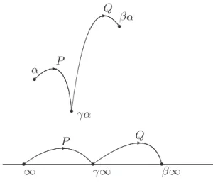
A central object in the theory of modular forms is the set of cusps P1(Q) = Q∪ {∞}. An element γ =¡a b c d ¢ ∈ SL2(Z) acts on P1(Q) by γ(z) = (_az+b cz+d if z6= ∞, a c if z =∞.

Also, note that if the denominator c or cz + d is 0 above, then γ(z) =∞ ∈ P1(Q).

The set of cusps for a congruence subgroup Γ is the set C(Γ) of Γ-orbits of P1(Q). (We will often identify elements of C(Γ) with a representative element from the orbit.) For example, the lemma below asserts that if Γ = SL2(Z), then there is exactly one orbit, so C(SL2(Z)) ={[∞]}.

Lemma 1.12. For any cusps α, β _{∈ P}1_{(Q) there exists γ} _{∈ SL}

2(Z) such

that γ(α) = β.

Proof. This is Exercise 1.8. ¤

Proposition 1.13. For any congruence subgroup Γ, the set C(Γ) of cusps is finite.

(20)

See [DS05,_{§3.8] and Algorithm 8.12 below for more discussion of cusps} and results relevant to their enumeration.

In order to define modular forms for general congruence subgroups, we next explain what it means for a function to be holomorphic on the extended

upper half plane

h∗ = h_{∪ P}1(Q).

See [Shi94, _{§1.3–1.5] for a detailed description of the correct topology} to consider on h∗. In particular, a basis of neighborhoods for α∈ Q is given by the sets{α} ∪ D, where D is an open disc in h that is tangent to the real line at α.

Recall from Section 1.2 that a weakly modular function f on SL2(Z) is

holomorphic at ∞ if its q-expansion is of the form P∞n=0anqn.

In order to make sense of holomorphicity of a weakly modular function f for an arbitrary congruence subgroup Γ at any α∈ Q, we first prove a lemma. Lemma 1.14. If f : h → C is a weakly modular function of weight k for

a congruence subgroup Γ and if δ _{∈ SL}2(Z), then f[δ]k is a weakly modular

function for δ−1Γδ.

Proof. If s = δ−1γδ_{∈ δ}−1Γδ, then

(f[δ]k₎[s]k _{= f}[δs]k _{= f}[δδ−1γδ]k _{= f}[γδ]k _{= f}[δ]k_.

¤ Fix a weakly modular function f of weight k for a congruence subgroup Γ, and suppose α _{∈ Q. In Section 1.2 we constructed the q-expansion of} f by using that f (z) = f (z + 1), which held since T =

µ 1 1 0 1 ¶

∈ SL2(Z).

There are congruence subgroups Γ such that T _{6∈ Γ. Moreover, even if we} are interested only in modular forms for Γ1(N ), where we have T ∈ Γ1(N )

for all N , we will still have to consider q-expansions at infinity for modular forms on groups δ−1_Γ₁_{(N )δ, and these need not contain T . Fortunately,}

TN = ¡1 N 0 1

¢

∈ Γ(N), so a congruence subgroup of level N contains TN_.

Thus we have f (z + H) = f (H) for some positive integer H, e.g., H = N always works, but there may be a smaller choice of H. The minimal choice of H > 0 such that¡1 H

0 1

¢

∈ δ−1Γδ, where δ(_{∞) = α, is called the width of the}

cusp α relative to the group Γ (see Section 1.4.1). When f is meromorphic

at infinity, we obtain a Fourier expansion

(1.3.2) f (z) =

∞

X

n=m

(21)

1.4. Remarks on Congruence Subgroups 7

in powers of the function q1/H _{= e}2πiz/H_{. We say that f is holomorphic at}

∞ if in (1.3.2) we have m ≥ 0.

What about the other cusps α _{∈ P}1(Q)? By Lemma 1.12 there is a γ _{∈ SL}2(Z) such that γ(∞) = α. We declare f to be holomorphic at the

cusp α if the weakly modular function f[γ]k _{is holomorphic at}∞.

Definition 1.15 (Modular Form). A modular form of integer weight k for a congruence subgroup Γ is a weakly modular function f : h _{→ C that is} holomorphic on h∗_{. We let M}_k_{(Γ) denote the space of weight k modular}

forms of weight k for Γ.

Proposition 1.16. If a weakly modular function f is holomorphic at a set of representative elements for C(Γ), then it is holomorphic at every element of P1(Q).

Proof. Let c1, . . . , cn ∈ P1(Q) be representatives for the set of cusps for

Γ. If α ∈ P1_{(Q), then there is γ} _{∈ Γ such that α = γ(c}

i) for some i. By

hypothesis f is holomorphic at ci, so if δ∈ SL2(Z) is such that δ(∞) = ci,

then f[δ]k _{is holomorphic at}_{∞. Since f is a weakly modular function for Γ,}

(1.3.3) f[δ]k _{= (f}[γ]k₎[δ]k _{= f}[γδ]k_.

But γ(δ(_{∞)) = γ(c}i) = α, so (1.3.3) implies that f is holomorphic at α. ¤

1.4. Remarks on Congruence Subgroups

Recall that a congruence subgroup is a subgroup of SL2(Z) that contains

Γ(N ) for some N . Any congruence subgroup has finite index in SL2(Z),

since Γ(N ) does. What about the converse: is every finite index subgroup of SL2(Z) a congruence subgroup? This is the congruence subgroup problem.

One can ask about the congruence subgroup problem with SL2(Z) replaced

by many similar groups. If p is a prime, then one can prove that every finite index subgroup of SL2(Z[1/p]) is a congruence subgroup (i.e., contains the

kernel of reduction modulo some integer coprime to p), and for any n > 2, all finite index subgroups of SLn(Z) are congruence subgroups (see [Hum80]).

However, there are numerous finite index subgroups of SL2(Z) that are not

congruence subgroups. The paper [Hsu96] contains an algorithm to decide if certain finite index subgroups are congruence subgroups and gives an example of a subgroup of index 12 that is not a congruence subgroup.

One can consider modular forms even for noncongruence subgroups. See, e.g., [Tho89] and the papers it references for work on this topic. We will not consider such modular forms further in this book. Note that modular sym-bols (which we define later in this book) are computable for noncongruence subgroups.

(22)

Finding coset representatives for Γ0(N ), Γ1(N ) and Γ(N ) in SL2(Z) is

straightforward and will be discussed at length later in this book. To make the problem more explicit, note that you can quotient out by Γ(N ) first. Then the question amounts to finding coset representatives for a subgroup of SL2(Z/N Z) (and lifting), which is reasonably straightforward.

Given coset representatives for a finite index subgroup G of SL2(Z), we

can compute generators for G as follows. Let R be a set of coset represen-tatives for G. Let σ, τ _{∈ SL}2(Z) be the matrices denoted by S and T in

(1.1.2). Define maps s, t : R _{→ G as follows. If r ∈ R, then there exists a} unique αr∈ R such that Grσ = Gαr. Let s(r) = rσα−1r . Likewise, there is

a unique βr such that Grτ = Gβr and we let t(r) = rτ βr−1. Note that s(r)

and t(r) are in G for all r. Then G is generated by s(R)∪ t(R). Proposition 1.17. The above procedure computes generators for G.

Proof. Without loss of generality, assume that I = (1 0

0 1) represents the

coset of G. Let g be an element of G. Since σ and τ generate SL2(Z), it is

possible to write g as a product of powers of σ and τ . There is a procedure, which we explain below with an example in order to avoid cumbersome notation, which writes g as a product of elements of s(R)_{∪ t(R) times a} right coset representative r∈ R. For example, if

g = στ2στ,

then g = Iστ2στ = s(I)yτ2στ for some y ∈ R. Continuing, s(I)yτ2στ = s(I)(yτ )τ στ = s(I)(t(y)z)τ στ for some z_{∈ R. Again,}

s(I)(t(y)z)τ στ = s(I)t(y)(zτ )στ =_{· · · .}

The procedure illustrated above (with an example) makes sense for arbitrary g and, after carrying it out, writes g as a product of elements of s(R)∪ t(R) times a right coset representative r∈ R. But g ∈ G and I is the right coset representative for G, so this right coset representative must be I. ¤ Remark 1.18. We could also apply the proof of Proposition 1.17 to write any element of G in terms of the given generators. Moreover, we could use it to write any element γ ∈ SL2(Z) in the form gr, where g∈ G and r ∈ R,

so we can decide whether or not γ∈ G.

1.4.1. Computing Widths of Cusps. Let Γ be a congruence subgroup of level N . Suppose α∈ C(Γ) is a cusp, and choose γ ∈ SL2(Z) such that

γ(∞) = α. Recall that the minimal h such that ¡1 h 0 1

¢

∈ γ−1_{Γγ is called}

the width of the cusp α for the group Γ. In this section we discuss how to compute h.

(23)

1.5. Applications of Modular Forms 9

Algorithm 1.19 (Width of Cusp). Given a congruence subgroup Γ of level N and a cusp α for Γ, this algorithm computes the width h of α. We assume

that Γ is given by congruence conditions, e.g., Γ = Γ0(N ) or Γ1(N ).

(1) [Find γ] Use the extended Euclidean algorithm to find γ∈ SL2(Z)

such that γ(∞) = α, as follows. If α = ∞, set γ = 1; otherwise, write α = a/b, find c, d such that ad_{− bc = 1, and set γ =}¡a b

c d

¢ . (2) [Compute Conjugate Matrix] Compute the following element of

Mat2(Z[x]): δ(x) = γ µ 1 x 0 1 ¶ γ−1.

Note that the entries of δ(x) are constant or linear in x.

(3) [Solve] The congruence conditions that define Γ give rise to four linear congruence conditions on x. Use techniques from elementary number theory (or enumeration) to find the smallest simultaneous positive solution h to these four equations.

Example 1.20. (1) Suppose α = 0 and Γ = Γ0(N ) or Γ1(N ). Then

γ =¡0 −1₁ ₀¢has the property that γ(_{∞) = α. Next, the congruence} condition is δ(x) = γ µ 1 x 0 1 ¶ γ−1= µ 1 0 −x 1 ¶ ≡ µ 1 _∗ 0 1 ¶ (mod N ).

Thus the smallest positive solution is h = N , so the width of 0 is N .

(2) Suppose N = pq where p, q are distinct primes, and let α = 1/p. Then γ =¡1 0_{p 1}¢sends_{∞ to α. The congruence condition for Γ}0(pq)

is δ(x) = γ µ 1 x 0 1 ¶ γ−1 = µ 1_{− px} x −p2_x _{px + 1} ¶ ≡ µ ∗ ∗ 0 _∗ ¶ (mod pq).

Since p2x_{≡ 0 (mod pq), we see that x = q is the smallest solution.} Thus 1/p has width q, and symmetrically 1/q has width p.

Remark 1.21. For Γ0(N ), once we enforce that the bottom left entry is 0

(mod N ) and use that the determinant is 1, the coprimality from the other two congruences is automatic. So there is one congruence to solve in the Γ0(N ) case. There are two congruences in the Γ1(N ) case.

1.5. Applications of Modular Forms

The above definition of modular forms might leave the impression that mod-ular forms occupy an obscure corner of complex analysis. This is not the case! Modular forms are highly geometric, arithmetic, and topological ob-jects that are of extreme interest all over mathematics:

(24)

(1) Fermat’s last theorem: Wiles’ proof [Wil95] of Fermat’s last theorem uses modular forms extensively. The work of Wiles et al. on modularity also massively extends computational methods for elliptic curves over Q, because many elliptic curve algorithms, e.g., for computing L-functions, modular degrees, Heegner points, etc., require that the elliptic curve be modular.

(2) Diophantine equations: Wiles’ proof of Fermat’s last theorem has made available a wide array of new techniques for solving cer-tain diophantine equations. Such work relies crucially on having access to tables or software for computing modular forms. See, e.g., [Dar97, Mer99, Che05, SC03]. (Wiles did not need a com-puter, because the relevant spaces of modular forms that arise in his proof have dimension 0!) Also, according to Siksek (personal communication) the paper [BMS06] would “have been entirely im-possible to write without [the algorithms described in this book].” (3) Congruent number problem: This ancient open problem is to determine which integers are the area of a right triangle with ra-tional side lengths. There is a potential solution that uses modular forms (of weight 3/2) extensively (the solution is conditional on truth of the Birch and Swinnerton-Dyer conjecture, which is not yet known). See [Kob84].

(4) Topology: Topological modular forms are a major area of current research.

(5) Construction of Ramanujan graphs: Modular forms can be used to construct almost optimal expander graphs, which play a role in communications network theory.

(6) Cryptography and Coding Theory: Point counting on elliptic curves over finite fields is crucial to the construction of elliptic curve cryptosystems, and modular forms are relevant to efficient algo-rithms for point counting (see [Elk98]). Algebraic curves that are associated to modular forms are useful in constructing and studying certain error-correcting codes (see [Ebe02]).

(7) The Birch and Swinnerton-Dyer conjecture: This central open problem in arithmetic geometry relates arithmetic proper-ties of elliptic curves (and abelian varieproper-ties) to special values of L-functions. Most deep results toward this conjecture use modu-lar forms extensively (e.g., work of Kolyvagin, Gross-Zagier, and Kato). Also, modular forms are used to compute and prove results about special values of these L-functions. See [Wil00].

(25)

1.6. Exercises 11

(8) Serre’s Conjecture on modularity of Galois representation: Let GQ = Gal(Q/Q) be the Galois group of an algebraic closure

of Q. Serre conjectured and many people have (nearly!) proved that every continuous homomorphism ρ : GQ → GL2(Fq), where

Fq is a finite field and det(ρ(complex conjugation)) =−1, “arises”

from a modular form. More precisely, for almost all primes p the coefficients ap of a modular (eigen-)form Panqn are congruent to

the traces of elements ρ(Frobp), where Frobp are certain special

elements of GQ called Frobenius elements. See [RS01] and [DS05,

Ch. 9].

(9) Generating functions for partitions: The generating functions for various kinds of partitions of an integer can often be related to modular forms. Deep theorems about modular forms then translate into results about partitions. See work of Ramanujan, Gordon, Andrews, and Ahlgren and Ono (e.g., [AO01]).

(10) Lattices: If L_{⊂ R}nis an even unimodular lattice (the basis matrix has determinant _{±1 and λ · λ ∈ 2Z for all λ ∈ L), then the theta} series

θL(q) =

X

λ∈L

qλ·λ

is a modular form of weight n/2. The coefficient of qm is the num-ber of lattice vectors with squared length m. Theorems and com-putational methods for modular forms translate into theorems and computational methods for lattices. For example, the 290 theorem of M. Bharghava and J. Hanke is a theorem about lattices, which asserts that an integer-valued quadratic form represents all posi-tive integers if and only if it represents the integers up to 290; it is proved by doing many calculations with modular forms (both theoretical and with a computer).

1.6. Exercises

1.1 Suppose γ =¡a b c d

¢

∈ GL2(R) has positive determinant. Prove that

if z _{∈ C is a complex number with positive imaginary part, then} the imaginary part of γ(z) = (az + b)/(cz + d) is also positive. 1.2 Prove that every rational function (quotient of two polynomials) is

a meromorphic function on C.

1.3 Suppose f and g are weakly modular functions for a congruence subgroup Γ with f 6= 0.

(a) Prove that the product f g is a weakly modular function for Γ. (b) Prove that 1/f is a weakly modular function for Γ.

(26)

(c) If f and g are modular functions, show that f g is a modular function for Γ.

(d) If f and g are modular forms, show that f g is a modular form for Γ.

1.4 Suppose f is a weakly modular function of odd weight k and level Γ0(N ) for some N . Show that f = 0.

1.5 Prove that SL2(Z) = Γ0(1) = Γ1(1) = Γ(1).

1.6 (a) Prove that Γ1(N ) is a group.

(b) Prove that Γ1(N ) has finite index in SL2(Z) (Hint: It contains

the kernel of the homomorphism SL2(Z)→ SL2(Z/N Z).)

(c) Prove that Γ0(N ) has finite index in SL2(Z).

(d) Prove that Γ0(N ) and Γ1(N ) have level N .

1.7 Let k be an integer, and for any function f : h∗ _{→ C and γ =}

¡_{a b}

c d

¢

∈ GL2(Q), set f[γ]k(z) = det(γ)k−1· (cz + d)−k · f(γ(z)).

Prove that if γ1, γ2 ∈ GL2(Z), then for all z∈ h∗ we have

f[γ1γ2]k_{(z) = ((f}[γ1]k₎[γ2]k_)(z).

1.8 Prove that for any α, β_{∈ P}1_{(Q), there exists γ} _{∈ SL}

2(Z) such that

γ(α) = β.

1.9 Prove Proposition 1.13, which asserts that the set of cusps C(Γ), for any congruence subgroup Γ, is finite.

1.10 Use Algorithm 1.19 to give an example of a group Γ and cusp α with width 2.

(27)

Chapter 2

Modular Forms of

Level

1

In this chapter we study in detail the structure of level 1 modular forms, i.e., modular forms on SL2(Z) = Γ0(1) = Γ1(1). We assume some complex

analysis (e.g., the residue theorem), linear algebra, and that the reader has read Chapter 1.

2.1. Examples of Modular Forms of Level 1

In this section we will finally see some examples of modular forms of level 1! We first introduce the Eisenstein series and then define ∆, which is a cusp form of weight 12. In Section 2.2 we prove the structure theorem, which says that all modular forms of level 1 are polynomials in Eisenstein series.

For an even integer k≥ 4, the nonnormalized weight k Eisenstein series is the function on the extended upper half plane h∗ = h∪ P1_{(Q) given by}

(2.1.1) Gk(z) = ∗ X m,n∈Z 1 (mz + n)k.

The star on top of the sum symbol means that for each z the sum is over all m, n_{∈ Z such that mz + n 6= 0.}

Proposition 2.1. The function Gk(z) is a modular form of weight k, i.e.,

Gk∈ Mk(SL2(Z)).

(28)

Proof. See [Ser73,_{§ VII.2.3] for a proof that G}k(z) defines a holomorphic

function on h∗_{. To see that G}_k _{is modular, observe that}

Gk(z + 1) = ∗ X 1 (m(z + 1) + n)k = ∗ X 1 (mz + (n + m))k = ∗ X 1 (mz + n)k,

where for the last equality we use that the map (m, n + m) 7→ (m, n) on Z_{× Z is invertible. Also,} Gk(−1/z) = ∗ X 1 (_{−m/z + n)}k = ∗ X zk (_{−m + nz)}k = zk ∗ X 1 (mz + n)k = z k_G k(z),

where we use that (n,_{−m) 7→ (m, n) is invertible.} ¤ Proposition 2.2. Gk(∞) = 2ζ(k), where ζ is the Riemann zeta function.

Proof. As z _{→ ∞ (along the imaginary axis) in (2.1.1), the terms that} involve z with m_{6= 0 go to 0. Thus}

Gk(∞) = ∗ X n∈Z 1 nk.

This sum is twice ζ(k) =P_n≥1_n1k, as claimed. ¤

2.1.1. The Cusp Form ∆. Suppose E = C/Λ is an elliptic curve over C, viewed as a quotient of C by a lattice Λ = Zω1+ Zω2, with ω1/ω2 ∈ h (see

[DS05,_{§1.4]). The Weierstrass ℘-function of the lattice Λ is} ℘ = ℘Λ(u) = 1 u2 + X k=4,6,8,... (k_{− 1)G}k(ω1/ω2)uk−2,

where the sum is over even integers k _{≥ 4. It satisfies the differential} equa-tion

(℘′)2 = 4℘3_{− 60G}4(ω1/ω2)℘− 140G6(ω1/ω2).

If we set x = ℘ and y = ℘′, the above is an (affine) equation of the form y2= ax3+bx+c for an elliptic curve that is complex analytically isomorphic to C/Λ (see [Ahl78, pg. 277] for why the cubic has distinct roots).

The discriminant of the cubic

4x3_{− 60G}4(ω1/ω2)x− 140G6(ω1/ω2)

is 16D(ω1/ω2), where

(29)

2.1. Examples of Modular Forms of Level1 15

Since D(z) is the difference of two modular forms of weight 12 it has weight 12. Moreover, D(_{∞) = (60G}4(∞))3− 27 (140G6(∞))2 = µ 60 32_{· 5}π 4 ¶3 − 27 µ 140_{· 2} 33_{· 5 · 7}π 6 ¶2 = 0,

so D is a cusp form of weight 12. Let

∆ = D

(2π)12.

Lemma 2.3. If z _{∈ h, then ∆(z) 6= 0.}

Proof. Let ω1 = z and ω2 = 1. Since E = C/(Zω1 + Zω2) is an elliptic

curve, it has nonzero discriminant ∆(z) = ∆(ω1/ω2)6= 0. ¤

Proposition 2.4. We have ∆ = q_·Q∞_n=1(1_{− q}n)24.

Proof. See [Ser73, Thm. 6, pg. 95]. ¤

Remark 2.5. SAGEcomputes the q-expansion of ∆ efficiently to high pre-cision using the command delta qexp:

sage: delta_qexp(6)

q - 24*q^2 + 252*q^3 - 1472*q^4 + 4830*q^5 + O(q^6)

2.1.2. Fourier Expansions of Eisenstein Series. Recall from (1.2.4) that elements f of Mk(SL2(Z)) can be expressed as formal power series in

terms of q(z) = e2πiz and that this expansion is called the Fourier expansion of f . The following proposition gives the Fourier expansion of the Eisenstein series Gk(z).

Definition 2.6 (Sigma). For any integer t≥ 0 and any positive integer n, the sigma function

σt(n) =

X

1≤d|n

dt

is the sum of the tth powers of the positive divisors of n. Also, let d(n) = σ0(n), which is the number of divisors of n, and let σ(n) = σ1(n). For

example, if p is prime, then σt(p) = 1 + pt.

Proposition 2.7. For every even integer k ≥ 4, we have Gk(z) = 2ζ(k) + 2· (2πi)k (k_{− 1)!} · ∞ X n=1 σ_k−1(n)qn.

(30)

Proof. See [Ser73, Section VII.4], which uses clever manipulations of series, starting with the identity

π cot(πz) = 1 z + ∞ X m=1 µ 1 z + m+ 1 z− m ¶ . ¤

From a computational point of view, the q-expansion of Proposition 2.7 is unsatisfactory because it involves transcendental numbers. To understand these numbers, we introduce the Bernoulli numbers Bnfor n≥ 0 defined by

the following equality of formal power series:

(2.1.2) x ex_{− 1} = ∞ X n=0 Bn xn n!. Expanding the power series, we have

x ex_{− 1}= 1− x 2 + x2 12− x4 720+ x6 30240− x8 1209600 +· · · .

As this expansion suggests, the Bernoulli numbers Bnwith n > 1 odd are 0

(see Exercise 1.2). Expanding the series further, we obtain the following table: B0 = 1, B1=− 1 2, B2 = 1 6, B4=− 1 30, B6 = 1 42, B8 =− 1 30, B10= 5 66, B12=− 691 2730, B14= 7 6, B16=− 3617 510, B18= 43867 798 , B20=− 174611 330 , B22= 854513 138 , B24=− 236364091 2730 , B26= 8553103 6 .

See Section 2.7 for a discussion of fast (analytic) methods for computing Bernoulli numbers.

We compute some Bernoulli numbers in SAGE:

sage: bernoulli(12) -691/2730 sage: bernoulli(50) 495057205241079648212477525/66 sage: len(str(bernoulli(10000))) 27706

A key fact is that Bernoulli numbers are rational numbers and they are connected to values of ζ at positive even integers.

(31)

2.2. Structure Theorem for Level 1 Modular Forms 17

Proposition 2.8. If k_{≥ 2 is an even integer, then}

ζ(k) =₋(2πi)

k

2_{· k!} · Bk.

Proof. This is proved by manipulating a series expansion of z cot(z) (see

[Ser73, Section VII.4]). ¤

Definition 2.9 (Normalized Eisenstein Series). The normalized Eisenstein

series of even weight k_{≥ 4 is}

Ek=

(k_{− 1)!} 2· (2πi)k · Gk.

Combining Propositions 2.7 and 2.8, we see that

(2.1.3) Ek =− Bk 2k + q + ∞ X n=2 σ_k−1(n)qn.

Warning 2.10. Our series Ek is normalized so that the coefficient of q

is 1, but often in the literature Ek is normalized so that the constant

coef-ficient is 1. We use the normalization with the coefcoef-ficient of q equal to 1, because then the eigenvalue of the nth Hecke operator (see Section 2.4) is the coefficient of qn. Our normalization is also convenient when considering congruences between cusp forms and Eisenstein series.

2.2. Structure Theorem for Level 1 Modular Forms

In this section we describe a structure theorem for modular forms of level 1. If f is a nonzero meromorphic function on h and w _{∈ h, let ord}w(f ) be

the largest integer n such that f (z)/(w_{− z)}n _{is holomorphic at w. If f =}

P_∞

n=manqn with am 6= 0, we set ord∞(f ) = m. We will use the following

theorem to give a presentation for the vector space of modular forms of weight k; this presentation yields an algorithm to compute this space.

Let Mk = Mk(SL2(Z)) denote the complex vector space of modular

forms of weight k for SL2(Z). The standard fundamental domain F for

SL2(Z) is the set of z∈ h with |z| ≥ 1 and |Re(z)| ≤ 1/2. Let ρ = e2πi/3.

Theorem 2.11 (Valence Formula). Let k be any integer and suppose f _∈ Mk(SL2(Z)) is nonzero. Then ord_∞(f ) +1 2ordi(f ) + 1 3ordρ(f ) + ∗ X w∈F ordw(f ) = k 12, where ∗ X w∈F

(32)

Proof. The proof in [Ser73, _{§VII.3] uses the residue theorem.} ¤ Let Sk = Sk(SL2(Z)) denote the subspace of weight k cusp forms for

SL2(Z). We have an exact sequence

0→ Sk→ Mk ι

∞

−−→ C

that sends f _{∈ M}k to f (∞). When k ≥ 4 is even, the space Mk contains

the Eisenstein series Gk, and Gk(∞) = 2ζ(k) 6= 0, so the map Mk → C is

surjective. This proves the following lemma.

Lemma 2.12. If k _{≥ 4 is even, then M}k = Sk⊕ CGk and the following

sequence is exact:

0_{→ S}k→ Mk ι

∞

−−→ C → 0.

Proposition 2.13. For k < 0 and k = 2, we have Mk= 0.

Proof. Suppose f _{∈ M}k is nonzero yet k = 2 or k < 0. By Theorem 2.11,

ord_∞(f ) +1 2ordi(f ) + 1 3ordρ(f ) + ∗ X w∈D ordw(f ) = k 12 ≤ 1 6.

This is not possible because each quantity on the left is nonnegative so whatever the sum is, it is too big (or 0, in which case k = 0). ¤ Theorem 2.14. Multiplication by ∆ defines an isomorphism M_k−12_{→ S}k.

Proof. By Lemma 2.3, ∆ is not identically 0, so because ∆ is holomorphic, multiplication by ∆ defines an injective map M_k−12֒→ Sk. To see that this

map is surjective, we show that if f _{∈ S}k, then f /∆∈ Mk−12. Since ∆ has

weight 12 and ord_∞(∆)_{≥ 1, Theorem 2.11 implies that ∆ has a simple zero} at _{∞ and does not vanish on h. Thus if f ∈ S}k and if we let g = f /∆,

then g is holomorphic and satisfies the appropriate transformation formula,

so g∈ Mk−12. ¤

Corollary 2.15. For k = 0, 4, 6, 8, 10, 14, the space Mk has dimension 1,

with basis 1, G4, G6, G8, G10, and G14, respectively, and Sk= 0.

Proof. Combining Proposition 2.13 with Theorem 2.14, we see that the spaces Mk for k≤ 10 cannot have dimension greater than 1, since otherwise

Mk′ 6= 0 for some k′ < 0. Also M

14 has dimension at most 1, since M2

has dimension 0. Each of the indicated spaces of weight _{≥ 4 contains the} indicated Eisenstein series and so has dimension 1, as claimed. ¤

Corollary 2.16. dim Mk=      0 if k is odd or negative, ⌊k/12⌋ if k _{≡ 2 (mod 12),} ⌊k/12⌋ + 1 if k 6≡ 2 (mod 12).

(33)

2.2. Structure Theorem for Level 1 Modular Forms 19

Proof. As we have already seen above, the formula is true when k _{≤ 12. By} Theorem 2.14, the dimension increases by 1 when k is replaced by k+12. ¤

Theorem 2.17. The space Mk has as basis the modular forms Ga4Gb6, where

a, b run over all pairs of nonnegative integers such that 4a + 6b = k.

Proof. Fix an even integer k. We first prove by induction that the modular forms Ga

4Gb6 generate Mk; the cases k ≤ 10 and k = 14 follow from the

above arguments (e.g., when k = 0, we have a = b = 0 and basis 1). Choose some pair of nonnegative integers a, b such that 4a + 6b = k. The form g = Ga₄Gb₆ is not a cusp form, since it is nonzero at_{∞. Now suppose f ∈ M}k

is arbitrary. Since g(_{∞) 6= 0, there exists α ∈ C such that f − αg ∈ S}k.

Then by Theorem 2.14, there is h _{∈ M}_k−12 such that f _{− αg = ∆ · h. By} induction, h is a polynomial in G4 and G6 of the required type, and so is ∆,

so f is as well. Thus

{Ga4Gb6 | a ≥ 0, b ≥ 0, 4a + 6b = k}

spans Mk.

Suppose there is a nontrivial linear relation between the Ga₄Gb₆ for a given k. By multiplying the linear relation by a suitable power of G4and G6,

we may assume that we have such a nontrivial relation with k_{≡ 0 (mod 12).} Now divide the linear relation by the weight k form Gk/6₆ to see that G3₄/G2₆ satisfies a polynomial with coefficients in C (see Exercise 2.4). Hence G3

4/G26

is a root of a polynomial, hence a constant, which is a contradiction since the q-expansion of G3₄/G2₆ is not constant. ¤ Algorithm 2.18 (Basis for Mk). Given integers n and k, this algorithm

computes a basis of q-expansions for the complex vector space Mk mod qn.

The q-expansions output by this algorithm have coefficients in Q.

(1) [Simple Case] If k = 0, output the basis with just 1 in it and terminate; otherwise if k < 4 or k is odd, output the empty basis and terminate.

(2) [Power Series] Compute E4 and E6 mod qnusing the formula from

(2.1.3) and Section 2.7. (3) [Initialize] Set b = 0.

(4) [Enumerate Basis] For each integer b between 0 and_{⌊k/6⌋, compute} a = (k _{− 6b)/4. If a is an integer, compute and output the basis} element E₄aEb₆ mod qn. When computing E₄a, find E₄m (mod qn) for each m ≤ a, and save these intermediate powers, so they can be reused later, and likewise for powers of E6.

(34)

Proof. This is simply a translation of Theorem 2.17 into an algorithm, since Ek is a nonzero scalar multiple of Gk. That the q-expansions have

coefficients in Q follows from (2.1.3). ¤

Example 2.19. We compute a basis for M24, which is the space with

small-est weight whose dimension is greater than 1. It has as basis E₄6, E₄3E₆2, and E4

6, whose explicit expansions are

E₄6 = 1 191102976000000+ 1 132710400000q + 203 44236800000q 2₊_{· · · ,} E₄3E₆2 = 1 3511517184000 − 1 12192768000q− 377 4064256000q 2₊_{· · · ,} E₆4 = 1 64524128256− 1 32006016q + 241 10668672q 2₊_{· · · .}

We compute this basis in SAGE as follows:

sage: E4 = eisenstein_series_qexp(4, 3) sage: E6 = eisenstein_series_qexp(6, 3) sage: E4^6 1/191102976000000 + 1/132710400000*q + 203/44236800000*q^2 + O(q^3) sage: E4^3*E6^2 1/3511517184000 - 1/12192768000*q - 377/4064256000*q^2 + O(q^3) sage: E6^4 1/64524128256 - 1/32006016*q + 241/10668672*q^2 + O(q^3)

In Section 2.3, we will discuss the reduced echelon form basis for Mk.

2.3. The Miller Basis

Lemma 2.20 (V. Miller). The space Sk has a basis f1, . . . , fd such that if

ai(fj) is the ith coefficient of fj, then ai(fj) = δi,j for i = 1, . . . , d. Moreover

the fj all lie in Z[[q]]. We call this basis the Miller basis for Sk.

This is a straightforward construction involving E4, E6 and ∆. The

following proof very closely follows [Lan95, Ch. X, Thm. 4.4], which in turn follows the first lemma of V. Miller’s thesis.

Proof. Let d = dim Sk. Since B4=−1/30 and B6= 1/42, we note that

F4=−

8 B4 · E4

(35)

2.3. The Miller Basis 21

and

F6 =−12

B6 · E6

= 1− 504q − 16632q2− 122976q3− 532728q4+· · ·

have q-expansions in Z[[q]] with leading coefficient 1. Choose integers a, b_≥ 0 such that

4a + 6b_{≤ 14} and 4a + 6b_{≡ k (mod 12),} with a = b = 0 when k ≡ 0 (mod 12), and let

gj = ∆jF62(d−j)+bF4a= µ ∆ F2 6 ¶j F₆2d+bF₄a, for j = 1, . . . , d.

Then it is elementary to check that gj has weight k

aj(gj) = 1 and ai(gj) = 0 when i < j.

Hence the gj are linearly independent over C, so form a basis for Sk. Since

F4, F6, and ∆ are all in Z[[q]], so are the gj. The fi may then be constructed

from the gj by Gauss elimination. The coefficients of the resulting power

series lie in Z because each time we clear a column we use the power series gj whose leading coefficient is 1 (so no denominators are introduced). ¤

Remark 2.21. The basis coming from Miller’s lemma is “canonical”, since it is just the reduced row echelon form of any basis. Also the set of all

integral linear combinations of the elements of the Miller basis are precisely

the modular forms of level 1 with integral q-expansion.

We extend the Miller basis to all Mk by taking a multiple of Gk with

constant term 1 and subtracting off the fi from the Miller basis so that the

coefficients of q, q2, . . . qdof the resulting expansion are 0. We call the extra basis element f0.

Example 2.22. If k = 24, then d = 2. Choose a = b = 0, since k _{≡ 0} (mod 12). Then g1= ∆F62 = q− 1032q2+ 245196q3+ 10965568q4+ 60177390q5− · · · and g2= ∆2 = q2− 48q3+ 1080q4− 15040q5+· · · . We let f2= g2 and f1 = g1+ 1032g2= q + 195660q3+ 12080128q4+ 44656110q5− · · · .

(36)

Example 2.23. When k = 36, the Miller basis including f0 is

f0 = 1 + 6218175600q4+ 15281788354560q5+· · · ,

f1 = q + 57093088q4+ 37927345230q5+· · · ,

f2 = q2+ 194184q4+ 7442432q5+· · · ,

f3 = q3− 72q4+ 2484q5+· · · .

Example 2.24. The SAGE command victor miller basis computes the Miller basis to any desired precision for a given k.

sage: victor_miller_basis(28,5) [ 1 + 15590400*q^3 + 36957286800*q^4 + O(q^5), q + 151740*q^3 + 61032448*q^4 + O(q^5), q^2 + 192*q^3 - 8280*q^4 + O(q^5) ]

Remark 2.25. To write f ∈ Mkas a polynomial in E4and E6, it is wasteful

to compute the Miller basis. Instead, use the upper triangular (but not echelon!) basis ∆jF₆2(d−j)+aF₄b, and match coefficients from q0 to qd.

2.4. Hecke Operators

In this section we define Hecke operators on level 1 modular forms and derive their basic properties. We will not give proofs of the analogous properties for Hecke operators on higher level modular forms, since the proofs are clearest in the level 1 case, and the general case is similar (see, e.g., [Lan95]).

For any positive integer n, let Xn= ½µ a b 0 d ¶ ∈ Mat2(Z) : a≥ 1, ad = n, and 0 ≤ b < d ¾ . Note that the set Xn is in bijection with the set of subgroups of Z2 of

index n, where¡a b c d

¢

corresponds to L = Z_{· (a, b) + Z · (0, d), as one can see} using Hermite normal form, which is the analogue over Z of echelon form (see Exercise 7.5).

Recall from (1.3.1) that if γ =¡a b c d

¢

∈ GL2(Q), then

f[γ]k _{= det(γ)}k−1_{(cz + d)}−k_{f (γ(z)).}

Definition 2.26 (Hecke Operator Tn,k). The nth Hecke operator Tn,k of

weight k is the operator on the set of functions on h defined by Tn,k(f ) =

X

γ∈Xn

(37)

2.4. Hecke Operators 23

Remark 2.27. It would make more sense to write Tn,k on the right, e.g.,

f_|Tn,k, since Tn,k is defined using a right group action. However, if n, m

are integers, then the action of Tn,k and Tm,k on weakly modular functions

commutes (by Proposition 2.29 below), so it makes no difference whether we view the Hecke operators of given weight k as acting on the right or left. Proposition 2.28. If f is a weakly modular function of weight k, then so is Tn,k(f ); if f is a modular function, then so is Tn,k(f ).

Proof. Suppose γ _{∈ SL}2(Z). Since γ induces an automorphism of Z2,

Xn· γ = {δγ : δ ∈ Xn}

is also in bijection with the subgroups of Z2 of index n. For each element δγ _{∈ X}n · γ, there is σ ∈ SL2(Z) such that σδγ ∈ Xn (the element σ

transforms δγ to Hermite normal form), and the set of elements σδγ is thus equal to Xn. Thus Tn,k(f ) = X σδγ∈Xn f[σδγ]k ₌ X δ∈Xn f[δγ]k _{= T} n,k(f )[γ]k.

A finite sum of meromorphic function is meromorphic, so Tn,k(f ) is weakly

modular. If f is holomorphic on h, then each f[δ]k _{is holomorphic on h for}

δ_{∈ X}n. A finite sum of holomorphic functions is holomorphic, so Tn,k(f ) is

holomorphic.

¤ We will frequently drop k from the notation in Tn,k, since the weight k

is implicit in the modular function to which we apply the Hecke operator. Henceforth we make the convention that if we write Tn(f ) and if f is

mod-ular, then we mean Tn,k(f ), where k is the weight of f .

Proposition 2.29. On weight k modular functions we have

(2.4.1) Tmn= TmTn if (m, n) = 1,

and

(2.4.2) Tpn = T_pn−1T_p − pk−1T_pn−2 if p is prime.

Proof. Let L be a subgroup of index mn. The quotient Z2_{/L is an abelian}

group of order mn, and (m, n) = 1, so Z2_{/L decomposes uniquely as a}

direct sum of a subgroup of order m with a subgroup of order n. Thus there exists a unique subgroup L′ such that L ⊂ L′ _{⊂ Z}2_{, and L}′ _{has index m}

in Z2. The subgroup L′ corresponds to an element of Xm, and the index n

subgroup L _{⊂ L}′ corresponds to multiplying that element on the right by some uniquely determined element of Xn. We thus have

(38)

i.e., the set products of elements in Xm with elements of Xn equal the

elements of Xmn, up to SL2(Z)-equivalence. Thus for any f , we have

Tmn(f ) = Tn(Tm(f )). Applying this formula with m and n swapped yields

the equality Tmn= TmTn.

We will show that Tpn + pk−1T_pn−2 = T_pT_pn−1. Suppose f is a weight k

weakly modular function. Using that f[

“ p 0 0 p ” ]k = (p2)k−1p−kf = pk−2f , we have X x∈Xpn f[x]k _{+ p}k−1 X x∈Xpn−₂ f[x]k ₌ X x∈Xpn f[x]k _{+ p} X x∈pXpn−₂ f[x]k_. Also TpTpn−1(f ) = X y∈Xp X x∈Xpn−1 (f[x]k₎[y]k ₌ X x∈Xpn−1·Xp f[x]k_.

Thus it suffices to show that Xpn disjoint union p copies of pX_pn−2 is equal

to X_pn−1 · X_p, where we consider elements with multiplicities and up to left

SL2(Z)-equivalence (i.e., the left action of SL2(Z)).

Suppose L is a subgroup of Z2 of index pn, so L corresponds to an element of Xpn. First suppose L is not contained in pZ2. Then the image

of L in Z2_/pZ2 _{= (Z/pZ)}2 _{is of order p, so if L}′ _{= pZ}2_{+ L, then [Z}2 _{: L}′_{] = p}

and [L : L′_{] = p}n−1_{, and L}′ _{is the only subgroup with this property. Second,}

suppose that L ⊂ pZ2 _{if of index p}n _{and that x} _{∈ X}

pn corresponds to L.

Then every one of the p + 1 subgroups L′ ⊂ Z2 _{of index p contains L. Thus}

there are p + 1 chains L_{⊂ L}′ _{⊂ Z}2 with [Z2 : L′] = p.

The chains L ⊂ L′ _{⊂ Z}2 _{with [Z}2 _{: L}′_{] = p and [Z}2 _{: L] = p}n−1 _{are in}

bijection with the elements of X_pn−1 · X_p. On the other hand the union of

Xpn with p copies of pX_pn−2 corresponds to the subgroups L of index pn,

but with those that contain pZ2 counted p + 1 times. The structure of the set of chains L _{⊂ L}′ _{⊂ Z}2 _{that we derived in the previous paragraph gives}

the result. ¤

Corollary 2.30. The Hecke operator Tpn, for prime p, is a polynomial in

Tp with integer coefficients, i.e., Tpn ∈ Z[T_p]. If n, m are any integers, then

TnTm= TmTn.

Proof. The first statement follows from (2.4.2) of Proposition 2.29. It then follows that TnTm = TmTnwhen m and n are both powers of a single prime p.

Combining this with (2.4.1) gives the second statement in general. ¤ Proposition 2.31. Let f =P_n∈Zanqn be a modular function of weight k.

Then Tn(f ) = X m∈Z   X 1≤d | gcd(n,m) dk−1a_mn/d2   qm_.

(39)

2.4. Hecke Operators 25

In particular, if n = p is prime, then

Tp(f ) = X m∈Z ³ amp+ pk−1am/p ´ qm, where am/p= 0 if m/p6∈ Z.

Proof. This is proved in [Ser73, §VII.5.3] by writing out Tn(f ) explicitly

and using thatP_0≤b<de2πibm/d _{is d if d}_{| m and 0 otherwise.} _¤

Corollary 2.32. The Hecke operators preserve Mk and Sk.

Remark 2.33. Alternatively, for Mkthe above corollary is Proposition 2.28,

and for Sk we see from the definitions that if f (∞) = 0, then Tnf also

vanishes at∞.

Example 2.34. Recall from (2.1.3) that

E4= 1

240+ q + 9q

2_{+ 28q}3_{+ 73q}4_{+ 126q}5_{+ 252q}6_{+ 344q}7₊_{· · · .}

Using the formula of Proposition 2.31, we see that

T2(E4) = (1/240 + 23· (1/240)) + 9q + (73 + 23· 1)q2+· · · .

Since M4 has dimension 1 and since we have proved that T2 preserves M4,

we know that T2 acts as a scalar. Thus we know just from the constant

coefficient of T2(E4) that

T2(E4) = 9E4.

More generally, for p prime we see by inspection of the constant coefficient of Tp(E4) that

Tp(E4) = (1 + p3)E4.

In fact Tn(Ek) = σk−1(n)Ek, for any integer n≥ 1 and even weight k ≥ 4.

Example 2.35. By Corollary 2.32, the Hecke operators Tn also preserve

the subspace Sk of Mk. Since S12 has dimension 1 (spanned by ∆), we

see that ∆ is an eigenvector for every Tn. Since the coefficient of q in the

q-expansion of ∆ is 1, the eigenvalue of Tn on ∆ is the nth coefficient of ∆.

Since Tnm = TnTm for gcd(n, m) = 1, we have proved the nonobvious fact

that the Ramanujan function τ (n) that gives the nth coefficient of ∆ is a multiplicative function, i.e., if gcd(n, m) = 1, then τ (nm) = τ (n)τ (m). Remark 2.36. The Hecke operators respect the decomposition Mk = Sk⊕

(40)

2.5. Computing Hecke Operators

This section is about how to compute matrices of Hecke operators on Mk.

Algorithm 2.37(Hecke Operator). This algorithm computes the matrix of

the Hecke operator Tn on the Miller basis for Mk.

(1) [Dimension] Compute d = dim(Mk)− 1 using Corollary 2.16.

(2) [Basis] Using Lemma 2.20, compute the echelon basis f0, . . . , fdfor

Mk (mod qdn+1).

(3) [Hecke operator] Using Proposition 2.31, compute for each i the image Tn(fi) (mod qd+1) .

(4) [Write in terms of basis] The elements Tn(fi) (mod qd+1) determine

linear combinations of

f0, f1, . . . , fd (mod qd).

These linear combinations are easy to find once we compute Tn(fi)

(mod qd+1_{), since our basis of f}

i is in echelon form. The linear

combinations are just the coefficients of the power series Tn(fi) up

to and including qd_.

(5) [Write down matrix] The matrix of Tn acting from the right

rela-tive to the basis f0, . . . , fd is the matrix whose rows are the linear

combinations found in the previous step, i.e., whose rows are the coefficients of Tn(fi).

Proof. By Proposition 2.31, the dth coefficient of Tn(f ) involves only adn

and smaller-indexed coefficients of f . We need only compute a modular form f modulo qdn+1 in order to compute Tn(f ) modulo qd+1. Uniqueness

in step (4) follows from Lemma 2.20 above. ¤

Example 2.38. We compute the Hecke operator T2on M12using the above

algorithm.

(1) [Compute dimension] We have d = 2_{− 1 = 1.}

(2) [Compute basis] Compute up to (but not including) the coefficient of qdn+1 = q1·2+1 = q3. As given in the proof of Lemma 2.20, we have

F4= 1 + 240q + 2160q2+· · · and F6 = 1− 504q − 16632q2+· · · .

Thus M12 has basis

F₄3= 1+720q +179280q2+_{· · · and ∆ = (F}₄3_−F₆2)/1728 = q_−24q2+_{· · · .} Subtracting 720∆ from F₄3 yields the echelon basis, which is

f0 = 1 + 196560q2+· · · and f1 = q− 24q2+· · · .

(41)

2.5. Computing Hecke Operators 27 sage: R.<q> = QQ[[’q’]] sage: F4 = 240 * eisenstein_series_qexp(4,3) sage: F6 = -504 * eisenstein_series_qexp(6,3) sage: F4^3 1 + 720*q + 179280*q^2 + O(q^3)

sage: Delta = (F4^3 - F6^2)/1728; Delta q - 24*q^2 + O(q^3)

sage: F4^3 - 720*Delta 1 + 196560*q^2 + O(q^3)

(3) [Compute Hecke operator] In each case letting an denote the nth

coefficient of f0 or f1, respectively, we have

T2(f0) = T2(1 + 196560q2+· · · ) = (a0+ 211a0)q0+ (a2+ 211a1/2)q1+· · · = 2049 + 196560q +· · · , and T2(f1) = T2(q− 24q2+· · · ) = (a0+ 211a0)q0+ (a2+ 211a1/2)q1+· · · = 0_{− 24q + · · · .} (Note that a_1/2 = 0.)

(4) [Write in terms of basis] We read off at once that

T2(f0) = 2049f0+ 196560f1 and T2(f1) = 0f0+ (−24)f1.

(5) [Write down matrix] Thus the matrix of T2, acting from the right

on the basis f0, f1, is T2 = µ 2049 196560 0 −24 ¶ .

As a check note that the characteristic polynomial of T2 is (x−2049)(x+24)

and that 2049 = 1 + 211 _{is the sum of the 11th powers of the divisors of 2.}

Example 2.39. The Hecke operator T2 on M36with respect to the echelon

basis is     34359738369 0 6218175600 9026867482214400 0 0 34416831456 5681332472832 0 1 194184 −197264484 0 0 −72 −54528     .

It has characteristic polynomial

(42)

where the cubic factor is irreducible.

The echelon form() command creates the space of modular forms but with basis in echelon form (which is not the default).

sage: M = ModularForms(1,36, prec=6).echelon_form() sage: M.basis() [ 1 + 6218175600*q^4 + 15281788354560*q^5 + O(q^6), q + 57093088*q^4 + 37927345230*q^5 + O(q^6), q^2 + 194184*q^4 + 7442432*q^5 + O(q^6), q^3 - 72*q^4 + 2484*q^5 + O(q^6) ]

Next we compute the matrix of the Hecke operator T2.

sage: T2 = M.hecke_matrix(2); T2

[34359738369 0 6218175600 9026867482214400]

[ 0 0 34416831456 5681332472832]

[ 0 1 194184 -197264484]

[ 0 0 -72 -54528]

Finally we compute and factor its characteristic polynomial.

sage: T2.charpoly().factor() (x - 34359738369) *

(x^3 - 139656*x^2 - 59208339456*x - 1467625047588864)

The following is a famous open problem about Hecke operators on mod-ular forms of level 1. It generalizes our above observation that the charac-teristic polynomial of T2 on Mk, for k = 12, 36, factors as a product of a

linear factor and an irreducible factor.

Conjecture 2.40 (Maeda). The characteristic polynomial of T2 on Sk is

irreducible for any k.

Kevin Buzzard observed that in several specific cases the Galois group of the characteristic polynomial of T2is the full symmetric group (see [Buz96]).

See also [FJ02] for more evidence for the following conjecture:

Conjecture 2.41. For all primes p and all even k _{≥ 2 the characteristic} polynomial of Tp,k acting on Sk is irreducible.