1
Carbon and land footprint time series of the
Netherlands - integrating data from the GTAP and
WIOD databases
Harry C. Wilting
PBL Netherlands Environmental Assessment Agency, Bilthoven, The Netherlands. E-mail: Harry.Wilting@pbl.nl
Abstract
This paper presents the results of an analysis of the carbon and land footprints of the Netherlands from 1995 to 2011. A multi-region input-output (MRIO) model was used for the calculation of these footprints. In recent years, several MRIO databases have become available all with their specific characteristics, advantages and drawbacks. In the MRIO model used, data from two of these databases, WIOD and GTAP, were integrated. The WIOD database enables the calculation of a consistent year-to-year time series. The GTAP database has more detail in regions and sectors than the WIOD database. Therefore, GTAP data were integrated into the WIOD data for a more detailed allocation of greenhouse gas (GHG) emissions and land use in agriculture.
Furthermore, the regional detail in the GTAP database was used for allocating land use and greenhouse gas emissions in the WIOD rest-of-the-world region to continents.
Greenhouse gas emissions related to Dutch consumption rose slightly with an annual increase of 0.3% in the period 1995-2011 with the rise in CO2 emissions as the main driver. Where the domestic emissions decreased the emissions related to imports for Dutch consumption rose. All WIOD countries outside the EU-27 showed an increase in greenhouse gas emissions for Dutch consumption. The land footprint increased with 0.4% a year as a result of a higher demand for crop and pasture land. The forest land footprint decreased in the period considered. By
integrating GTAP data into the WIOD tables, a breakdown of the Dutch footprints into continents became visible. Europe, Central and South America and Asia showed the largest contributions in the Dutch land footprint.
2
Disclaimer: The analysis presented in this paper is still work in progress and not all results are
available yet. Results presented may change in the final version of the paper, so citation of figures is not recommended.
Introduction
Dutch government is as part of its sustainability strategy increasingly interested in the impacts of domestic production and consumption on the environment and biodiversity abroad (Dutch Government, 2011). The government likes to have time series of biodiversity footprint indicators for monitoring purposes and asked Statistics Netherlands and PBL to develop and update such indicators. Important indicators of such a set of biodiversity indicators are a carbon and land footprint indicator. These footprint indicators depict the embodied greenhouse gas (GHG) emissions and land use in final demand (consumption of goods and services and investments)1.
The common methodology for calculating footprint indicators at the national level is input-output analysis (Wiedmann et al, 2009). The fact that recently several multi-regional input-input-output (MRIO) databases came available has facilitated and accelerated the calculation of footprints for various countries. One of the advantages of the use of MRIO data is that the impact abroad can be allocated to individual countries or regions. Two examples of MRIO databases2 that were used for footprint calculations regularly are GTAP (GTAP, 2014) and WIOD (Timmer, 2012). Calculations with GTAP data were carried out for groups of countries (Peters and Hertwich, 2008) and individual countries like New Zealand (Andrew and Forgie, 2008), the Netherlands (Wilting, 2012) and the UK (Wiedmann et al., 2010). Arto et al. (2012) calculated time series of environmental footprint indicators for 40 countries by using WIOD data.
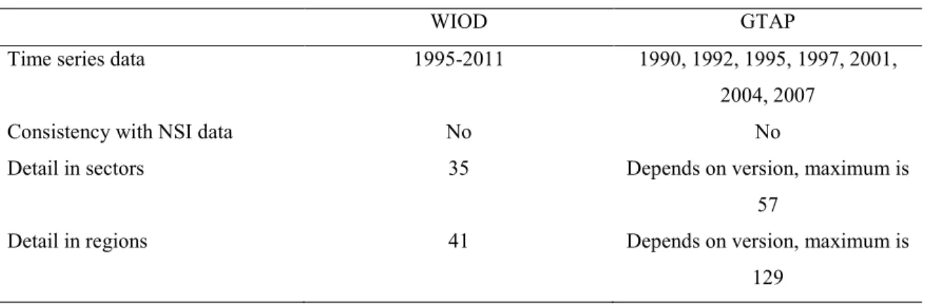
Both GTAP and WIOD have specific characteristics, advantages and disadvantages (Table 1). WIOD has a consistent time series for the period 1995-2009 (and a recent update to 2011), which enables comparisons over time. New GTAP versions are published every two or three years, but the data in different versions are poorly comparable. For comparisons with ‘official’ national statistics it is useful that the input-output data used match with data in the national accounts published by National Statistical Institutes (NSIs). Data in GTAP and WIOD differ from the original data published by NSIs; especially the GTAP input-output data for the Netherlands differ substantially from the original IO data for the Netherlands (compiled by Statistics
1 These indicators should not be confused with the ecological footprint and related carbon footprint, so all
land use figures apply to physical areas. .
2 The global MRIO databases EORA (Lenzen et al., 2013) and Exiopol (Tukker et al., 2013) are not
3
Netherlands and the Agricultural Economics Research Institute) on which the GTAP data were based. These differences are caused by the adjusting and updating procedures applied by the GTAP consortium in order to balance import and export flows between countries (McDougall, 2008). The WIOD data are more close to the official data for the Netherlands, but do not completely match either. Especially import and export data show substantial differences. The numbers of sectors and regions in WIOD are limited compared to GTAP. WIOD consists of only one aggregated agricultural sector. This is a relevant issue in compiling carbon and land footprints, since non-CO2 emissions and land use are significantly related to agriculture. Contrary, the GTAP databases are far more detailed by distinguishing 14 subsectors in
agriculture. The regional detail in WIOD is also less detailed than the regional detail in GTAP. Calculations based on WIOD data show that the share of the Rest of the world (RoW) region in the foreign part of the Dutch carbon and land footprint is about 25% and 50%, respectively. Furthermore, a breakdown of the footprints into continents is not possible. The number of countries and regions in the latest GTAP version (GTAP 8) is 129. Given the characteristics of both databases, WIOD and GTAP might complement each other.
Table 1 Characteristics of the WIOD and GTAP databases.
WIOD GTAP
Time series data 1995-2011 1990, 1992, 1995, 1997, 2001,
2004, 2007
Consistency with NSI data No No
Detail in sectors 35 Depends on version, maximum is
57
Detail in regions 41 Depends on version, maximum is
129
In order to compile a time series of Dutch footprints, the availability of a data series that is consistent in time is a crucial aspect. Therefore we took the WIOD as a starting point. However, the standard WIOD dataset can be adjusted and extended at the aspects discussed above: 1) The domestic data for the Netherlands in WIOD do not match completely with the data
published by Statistics Netherlands. Hoekstra et al. (2013) developed the so-called SNAC3 method to cope with this problem. This method in which national data from the NSI were integrated in WIOD is beyond the scope of this paper.
4
2) Sectoral detail. WIOD consists of one aggregated agricultural sector. This is a real problem in the calculation of carbon and land footprints, since non-CO2 greenhouse gas emissions and land use mainly take place in agriculture. Since agriculture is more detailed in GTAP, these data were used to disaggregate the agricultural sector in WIOD.
3) Regional detail. The role of the Rest of the world in WIOD is substantial in calculating carbon and land footprints and partly covers several continents. GTAP data were used to disaggregate the Rest of the world in WIOD in order to refine allocations of footprints to regions and enable allocation to continents.
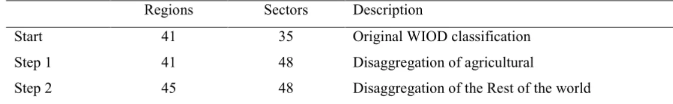
Summarizing, the original WIOD MRIO tables were disaggregated in two steps in order to obtain the data for the MRIO model used in this paper for calculating the Dutch footprints (Table 2).
Table 2 Number of sectors and regions in the original WIOD database and after applying two disaggregation steps.
Regions Sectors Description
Start 41 35 Original WIOD classification
Step 1 41 48 Disaggregation of agricultural
Step 2 45 48 Disaggregation of the Rest of the world
Methodology and data
Environmental footprint
The calculation of the carbon and land footprints related to Dutch consumption was carried out by using MRIO analysis. The general MRIO model for calculating the environmental pressures as a result of final demand, Ei, in a certain region i is:
Ei = d (I – A)-1 yi + Di (1)
With
[
d
1d
n]
d
=
di is a row vector of direct environmental pressure intensities ofregion i (depicting the pressure of one unit of production for all sectors)
A
A
A
A
A
=
nn n n
1 111 Aii is the matrix of domestic input coefficients of region i, Aij, i≠j is the matrix of import coefficients of region j importing from region i,
5
I Matrix I is the identity matrix; (I – A)-1 is the Leontief inverse
matrix.
=
ni i iy
y
y
1 ,yii is the vector of domestic final demand of region i, and yji, j≠i is
the vector of imported final demand of region i importing from region j.
Di Di is the direct pressure of final demand in region i.
The input-output formalism also enables the calculation of a breakdown of the national footprints into regions and sectors of origin as well as the breakdown into consumption categories. More comprehensive descriptions are available in input-output literature (see e.g. Arto et al., 2012).
Overview of the data sources
The MRIO model requires economic input-output data and environmental data from several sources (Table 3). For the disaggregation of the WIOD MRIO tables and environmental data, data from other sources was used.
Table 3 Start data and data used in the two disaggregation steps.
MRIO data GHG data Land use data
Start WIOD WIOD WIOD
Step 1 WIOD + GTAP WIOD + Edgar + GTAP +
UNFCCC
FAO, FRA
Step 2 WIOD + GTAP WIOD + Edgar + GTAP +
UNFCCC
FAO, FRA
Economic data
Input-output data were obtained from WIOD, which describes the global economy in the period 1995-2011 (Timmer, 2012). The database contains input-output data at the level of 35 sectors in 40 countries and a region called Rest of the world (RoW). All MRIO tables (World Input-Output Tables, Released November 2013) for the period 1995-2011 were downloaded from the WIOD website. Final demand categories were aggregated to one final demand vector per region.
Totally, there are five versions of the GTAP database that include data for the period 1995-2009, viz. GTAP 4 (base year 1995), GTAP 5 (1997), GTAP 6 (2001), GTAP 7 (2004) and GTAP 8 (2004 and 2007). For the spatial and sectoral disaggregation of the WIOD data, three
6
GTAP versions were used. We used version 5.44 (
Dimaranan and McDougall, 2002)
, version 6 (Dimaranan, 2005)
and version 8 (Narayanan, 2012)
to obtain data for the base years 1997, 2001, 2004 and 2007, respectively. All versions distinguish 57 sectors, but the number of regions increases with higher version numbers. GTAP 8 is the most detailed version with 129 regions. We did not use version 4, because of the lack of detail in the number of regions; it did not include the Netherlands as a separate region. Complete MRIO tables were constructed at the mostdetailed regional and sectoral level for each of the four GTAP base years by using the method described by Peters et al. (2011).
Greenhouse gas emission data
Data on greenhouse gas emissions (CO2, CH4 and N2O) for the 41 WIOD regions were derived from WIOD (Emissions to air by sector and pollutant). We adjusted these data at one point. In WIOD, methane emissions related to landfills are allocated to the government sector (sector 34). Usually in NAMEAs these emissions are not allocated to industrial sectors or households, but are reported separately. Therefore, we moved the main part (99%) of the methane emissions allocated to the government sector to direct emissions of final demand in all regions.
More detailed data on greenhouse gas emissions at the level of GTAP sectors and regions, which were used for the disaggregation steps, were obtained from several databases. CO2 emission data were obtained from the GTAP database versions;GTAP-E Flexagg Data Base Package for version 8 (
Narayanan, 2012) and the
GTAP/EPA database for previous years (Lee, 2005). Data on CH4 and N2O emissions were retrieved from the EDGAR database, version 4.2 (JRC and PBL, 2010) that consists of emissions by country and main source category.The
EDGAR data on emissions were allocated to different crop and livestock sectors in
GTAP (Table 4).
Furthermore, emissions in GTAP livestock sectors were further disaggregated by using UNFCCC data on greenhouse gas emissions of specific animal categories (UNFCCC, 2013).
7
Table 4 Allocation of EDGAR data on CH4 and N2O emissions to 14 GTAP agricultural subsectors.
CH4 N2O
1 Paddy rice Rice cultivation Direct soil emissions, manure
management
2 Wheat Direct soil emissions, manure
management
3 Cereal grains nec Direct soil emissions, manure
management
4 Vegetables, fruit, nuts Direct soil emissions, manure
management
5 Oil seeds Direct soil emissions, manure
management
6 Sugar cane, sugar beet Direct soil emissions, manure
management
7 Plant-based fibers Direct soil emissions, manure
management
8 Crops nec Direct soil emissions, manure
management
9 Bovine cattle, sheep and goats, horses
Enteric fermentation, manure management
Manure in pasture
10 Animal products nec Manure management Manure in pasture
11 Raw milk Enteric fermentation, manure
management
Manure in pasture
12 Wool, silk-worm cocoons manure management Manure in pasture
13 Forestry
14 Fishing
Nec: not else classified.
Land-use data
WIOD consists of data on land use divided in arable and permanent crop area, pasture area and forest area (Land use by type and sector). However, we did not use these data in the land footprint calculations, since these data would give an overestimation of the footprint. E.g. all forest area in the world was allocated to agriculture in WIOD, although only part of the forests is used for production purposes. For our model, we obtained data on the detailed land use in the GTAP agricultural subsectors from FAOStat (FAO, 2013a).
Detailed data on crop area (harvested area) for more than 150 crops and 238 countries were aggregated to 8 crop sectors and 129 regions (according to the GTAP 8 classification) for the GTAP base years. Land use for pasture was directly obtained from FAOStat and assigned to the livestock sectors in GTAP on the basis of production values of these sectors. Pigs and chicken
8
are more often than bovine cattle, sheep and goats kept in stables. Therefore, we assumed that the land use intensity (land use per unit of production) of the sector ‘other animal products’ is lower than the intensity in the other livestock sectors; only 25% of the production value of this sector was used in the weighing. No correction was made yet for extensive or intensive use of the pasture land, although there are huge differences in local land-use intensities between countries.
Land use for forestry products was estimated from the FRA dataset (FAO, 2013b) by combining data on removals of wood products (industrial roundwood and wood fuel), growing stock volumes per hectare and a 25-year rotation period. Data were available for 1990, 2000 and 2005; data for other years were based on interpolation. Built-up land, i.e. urban land and land for infrastructure, was not included in the Dutch land footprint yet.
Disaggregation of agriculture
The WIOD agricultural sector is disaggregated in 14 subsectors corresponding with the 14 agricultural commodity groups in the GTAP database (see Table 4).In preparation of the disaggregation, the GTAP-based MRIO tables for all GTAP base years were aggregated to two levels; 1) the original WIOD classification with one agricultural sector; 2) the WIOD
classification extended with the detailed agricultural subsectors. On the basis of these two GTAP-based tables, shares were derived presenting the share of agricultural subsectors in total
agriculture. These shares concern cells in the intermediate matrix, the final demand matrix and total production. For the non-GTAP base years, shares of agricultural subsectors were derived by interpolating and extrapolating the shares in the GTAP base years. All these shares were used to disaggregate the rows and columns corresponding to agriculture in the WIOD MRIO tables by maintaining the WIOD totals. In disaggregating the intermediate matrices, first the cells in rows were disaggregated and after that the cells in columns. The application of the procedures mentioned resulted in a WIOD-based MRIO table of 41 regions and 48 sectors per region. Final demand still consists of one vector per region. No balancing of the tables was carried out yet, but might be necessary when differences between column and row totals deviate too much.
The greenhouse gas emission data for the GTAP regions were aggregated to the WIOD regions. Shares of emissions of the agricultural subsectors in total emissions in agriculture per region were derived from these aggregated GTAP data. These shares were used to disaggregate the WIOD greenhouse gas emissions of agriculture maintaining the WIOD greenhouse gas emission totals. Data on land use in the agricultural subsectors in the GTAP regions were aggregated to the WIOD regions and directly applied in the footprint calculation.
9 Disaggregation of the Rest of the world
The second step in the disaggregation of the WIOD data is the disaggregation of the WIOD RoW-region. The WIOD RoW-region was disaggregated in five subregions, viz. Rest of Oceania, Rest of America, Rest of Asia, Rest of Europe and Africa. In preparation of the disaggregation of the RoW-region, the GTAP MRIO tables were aggregated to two levels; 1) the WIOD classification extended with the detailed agricultural subsectors with one RoW-region, i.e. the classification after disaggregation step 1; 2) the WIOD classification extended with the detailed agricultural subsectors with detailed RoW-subregions. On the basis of these two GTAP-based tables for each GTAP year, shares were derived at the level of individual matrix and vector elements presenting the shares of the five RoW-subregions in the total RoW-region. These shares obtained from the GTAP tables were applied to disaggregate the WIOD RoW-region into five subregions. Data on greenhouse gas emissions and land use in these five regions were derived from the GTAP data on emissions and land use per region.
Preliminary results
First, we discuss the outcomes for the carbon footprint and then the outcomes for the land footprint. These outcomes are preliminary, since only disaggregation step 1 was applied for all years in the period 1995-2011 yet. Disaggregation step 2 was just carried out for the year 2007.
Carbon footprint
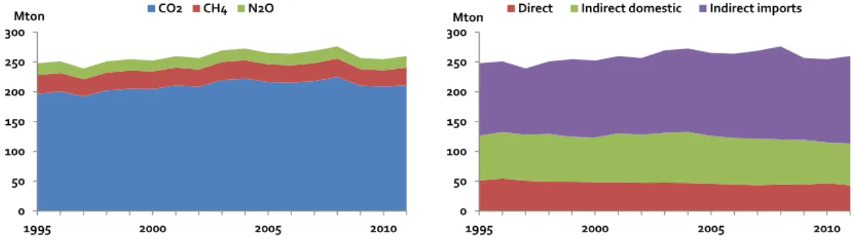
The carbon footprint of the Netherlands slightly increased in the period 1995-2008 up to 276 megaton of CO2 equivalents5 (Figure 1, left). In 2009 and following years, the carbon footprint stayed at a 6-8% lower level due to lower consumption in these years. Where the emissions of CH4 and N2O decreased, CO2 emissions increased with 0.5% per year in the period 1995-2009. Especially the foreign part of the carbon footprint according to greenhouse gas emissions embodied in imports increased showing a shift from domestic emissions to foreign emissions (Figure 1, right). The decrease in the direct emissions of private and public consumers was mainly the result of lower methane emissions of landfills.
5 Based on Global Warming Potentials relative to CO
10
Figure 1 Carbon footprint of the Netherlands in the period 1995-2011. Shares of individual greenhouse gases (left) and contributions of direct and indirect emissions (right).
Greenhouse gas emissions related to Dutch consumption were broken down to 48 consumption categories corresponding to the 48 sectors involved in the disaggregated MRIO tables. We aggregated the outcomes to ten aggregated categories summed up over all regions. Emissions were considered up to the final producing sector delivering to final demand. From a consumption perspective, services have the highest share in the Dutch carbon footprint (Figure 2, left), since services have a high share in Dutch consumption. Other consumption categories with relatively high supply-chain emissions consists of products form the energy sector, food industry and other manufacturing. These consumption categories have relatively large emission multipliers
representing the supply-chain emissions per unit of demand.
Figure 2 Breakdown of the carbon footprint into consumption categories (presented as sectors supplying goods and services to final demand) (left) and into sectors of origin where emissions actually took place (right).
The MRIO framework also gives insights in the sectors where greenhouse gases related to Dutch carbon footprint were emitted. The energy sector was the main contributor to the carbon footprint
0 50 100 150 200 250 300 1995 2000 2005 2010
Mton CO2 CH4 N2O
0 50 100 150 200 250 300 1995 2000 2005 2010
Mton Direct Indirect domestic Indirect imports
0 50 100 150 200 250 300 1995 2000 2005 2010 Mton Direct Services Transport Trade Energy Other industry Food industry Basic industry Mining Agriculture 0 50 100 150 200 250 300 1995 2000 2005 2010 Mton
11
(Figure 2, right), since electricity is essential to many production processes. The share of the energy sector in the Dutch carbon footprint even rose 3 percentage points to more than 30%. Especially non-CO2 greenhouse gas emissions in agriculture had a significant contribution to the Dutch carbon footprint as well. The share of direct greenhouse gas emissions from households, government consumption and landfills, declined with more than 4 percentage points in the period 1995-2011.
The disaggregation of agricultural (step 1) had a substantial effect on the calculated non-CO2 greenhouse gas emissions in agriculture. Total methane emitted in agriculture was about 10-20% lower compared to the outcomes of a pure WIOD-based calculation of the Dutch carbon footprint (Figure 3). N2O emissions in global agriculture based on the disaggregated tables were 5-10% lower than calculated by using WIOD without disaggregation. So, calculations based on the aggregated agricultural sector overestimate the Dutch carbon footprint.
Figure 3 Methane and nitrous oxide emissions in global agriculture contributing to the Dutch carbon footprint. Figures calculated with the original WIOD tables (line) and the disaggregated tables (shaded areas).
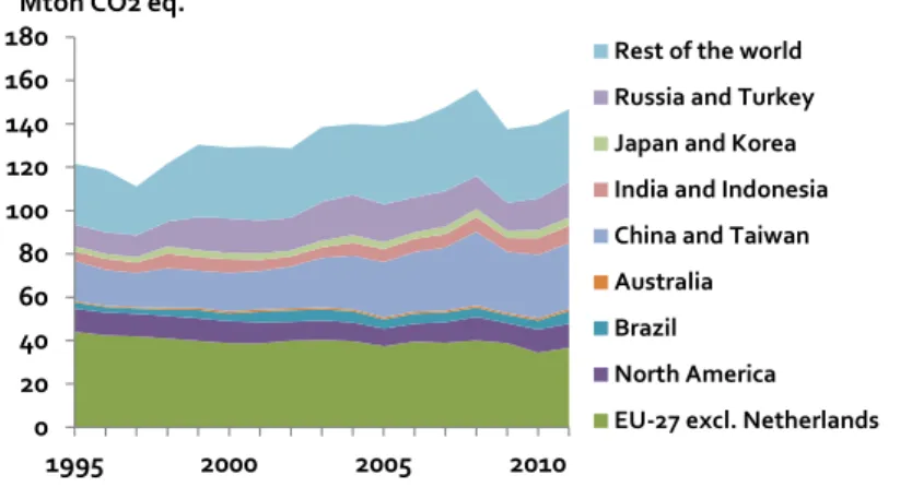
Since 1999, more than 50% of greenhouse gases that were allocated to Dutch consumption have been emitted abroad, as they were related to the production of imported goods and services (see Figure 1). Greenhouse gases embodied in imports were mainly emitted in other EU-27 countries, China and the Rest of the world (Figure 4). Contributions in all regions except the EU-27
increased in the period 1995-2011. Greenhouse gas emissions as a result of Dutch consumption almost doubled in Brazil, Korea and Indonesia.
0 2 4 6 8 10 12 14 16 18 1995 2000 2005 2010
Mton CO2 eq. CH4
Other animal products Raw milk
Bovine cattle, sheep and goats, horses Paddy rice and other crops Total agriculture WIOD 0 2 4 6 8 10 12 14 16 18 1995 2000 2005 2010 N2O
12
Figure 4 Greenhouse gas emissions embodied in imports per world region, 1995-2011.
Greenhouse gas emissions in the Rest of the world are about 25% of greenhouse gases embodied in imports. For further insights in the spatial allocation of these emissions we disaggregated this region in the WIOD tables (step 2). However, at the moment of writing this paper, calculations were carried out for just one year, viz. 2007. The calculation of the whole time series will be done at a later moment. For most regions and sectors, the detailed outcomes for 2007 based on two disaggregation steps were very close to the outcomes based on one disaggregation step presented before. The disaggregation of the Rest of the world gives more detailed insights in the allocation of greenhouse gas emissions to continents. By far most of the ‘foreign’ greenhouse gases related to the Dutch carbon footprint were emitted in Europe and Asia. The region Central and South America has relatively high contributions in the CH4 and N2O footprints due to the large production of agricultural products for Dutch consumption.
Figure 5 Breakdown of the Dutch carbon footprint (indirect emissions) into greenhouse gases and world regions by origin, 2007.
0 20 40 60 80 100 120 140 160 180 1995 2000 2005 2010 Mton CO2 eq.
Rest of the world Russia and Turkey Japan and Korea India and Indonesia China and Taiwan Australia Brazil North America EU-27 excl. Netherlands
0 20 40 60 80 Netherlands Rest of Europe North America CS America Africa Asia Oceania Mton CO2 eq CO2 CH4 N2O
13 Land footprint
The land footprint of the Netherlands slightly increased in the period 1995-20096 up to 20.5 million hectares (Figure 6, left), which corresponds to 1.25 hectares per capita. The land footprint increased with 0.4% a year as a result of a higher demand for crop and pasture land. The forest land footprint decreased in the period considered. More than 97% of the land footprint consists of land use abroad embodied in imports (Figure 6, right). This share even rose in the period
considered. Direct land use of private and public consumers, like built-up land for houses and infrastructure, was not included in the analysis. Inclusion will increase the domestic share in the land footprint.
Figure 6 Land footprint of the Netherlands in the period 1995-2009. Shares of land types (left) and contributions of domestic and imported indirect land use (right)7.
Land use related to consumption of products from the food industry, agriculture, services and other industry covers more than 80% of the Dutch land footprint (Figure 7). Production in the latter two sectors has a high requirement of forest land related products like paper and building materials.
6 We present the outcomes for period 1995-2009, since the FAO data on detailed land use were not
available in the required format for the years 2010-2011.
7 The considerable decrease in the land footprint in 1997 might be an artefact of the WIOD tables for that
year. 0 5 10 15 20 25 1995 2000 2005
million ha Crop land Pasture land Forest land
0 5 10 15 20 25 1995 2000 2005
14
Figure 7 Contributions of sectors supplying goods and services to final demand in the land footprint. Almost all land use required for Dutch consumption was for agricultural purposes abroad, as it is related to the production of imported goods and services. About half of the land use was in the Rest of the world, which consists of countries all over the world. Other important contributors were the EU-27, Brazil and China (Figure 8).
Figure 8 Land use embodied in imports per world region, 1995-2009.
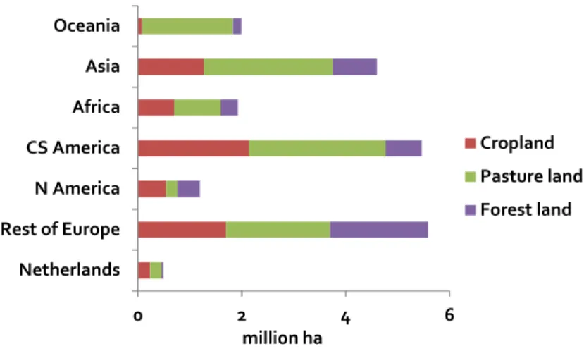
The disaggregation of the Rest of the world shows the breakdown of the Dutch land footprint into continents in 2007 (Figure 9). Europe, Central and South America and Asia are the main
contributors. Oceania, Africa and North America have a lower share, but the land use as a result of Dutch consumption in these continents is still far more higher than the domestic part of the footprint. 0 5 10 15 20 25 1995 2000 2005 million ha Direct Services Transport Trade Energy Other industry Food industry Basic industry Mining Agriculture 0 5 10 15 20 25 1995 2000 2005 million ha
Rest of the world Russia and Turkey Japan and Korea India and Indonesia China and Taiwan Australia Brazil North America EU-27 excl. Netherlands
15
Figure 9 Land use embodied in imports for Dutch consumption per world region, 2007.
Discussion
p.m.
Conclusions
The integration of GTAP data in WIOD provides more detailed outcomes of footprints. The disaggregation of agriculture showed that the calculation with one aggregated agricultural sector in WIOD overestimates Dutch carbon footprint. Furthermore, the disaggregation of Rest of the world in WIOD enabled a breakdown of the carbon and land footprint into continents.
Both the Dutch carbon and land footprint increased slightly in the period 1995-2009, although there was a fall back to lower levels in 2009 due to lower demand. More than 50% of the Dutch carbon footprint and almost total land footprint is related to imports. Especially, the emissions and land use in non-European countries are increasing indicating the further globalization of the world.
References
Andrew, R. and V. Forgie (2008). A three-perspective view of greenhouse gas emission responsibilities in New Zealand. Ecological Economics 68, 194-204.
Arto, I., Genty, A., Rueda-Cantuche, J.M., Villanueva, A., Andreoni, V., (2012) Global
Resources Use and Pollution, Volume 1 / Production, Consumption and Trade (1995-2008). European Commission, Joint Research Centre, Institute for Prospective Technological Studies (JRC-IPTS), Luxembourg.
0 2 4 6 Netherlands Rest of Europe N America CS America Africa Asia Oceania million ha Cropland Pasture land Forest land
16
Dimaranan, Betina V. and Robert A. McDougall, Ed. 2002. Global Trade, Assistance, and Production: The GTAP 5 Data Base, Center for Global Trade Analysis, Purdue University. Available online at: http://www.gtap.agecon.purdue.edu/databases/v5/v5_doco.asp
Dimaranan, Betina V., Ed. 2006. Global Trade, Assistance, and Production: The GTAP 6 Data Base, Center for Global Trade Analysis, Purdue University. Available online at:
http://www.gtap.agecon.purdue.edu/databases/v6/v6_doco.asp
Dutch Government (2011), Agenda Duurzaamheid; een groene groeistrategie voor Nederland, Joint letter of the State Secretary of Infrastructure and the Environment, State Secretary of Foreign Affairs and the Minister of Economic Affairs.
FAO (2013a), FAOSTAT, Food and Agriculture Organization of the United Nations, Rome,
http://faostat3.fao.org/faostat-gateway/go/to/home/E
FAO (2013b), Global Forest Resources Assessment 2005, Food and Agriculture Organization of the United Nations, Rome, http://www.fao.org/forestry/fra/fra2005/en/
GTAP (2014), GTAP databases, Global Trade Analysis Project, Center for Global Trade Analysis, Department of Agricultural Economics, Purdue University,
https://www.gtap.agecon.purdue.edu/databases/default.asp
Hoekstra, R., Edens, B., Zult, D., Wilting, H., Lemmers, O., Wu, R. en Goel, A. (2013),
Producing Carbon Footprints that are Consistent to the Dutch National and Environmental Accounts, paper presented at the 21st International Input-Output Conference, July 9-12th 2013, Kitakyushu, Japan and at the Workshop on the Wealth of Nations in a Globalizing World, July 18-19th 2013, Groningen, The Netherlands.
Houghton, J.T., Meira Filho, L.G., Callander, B.A., Harris, N., Kattenberg, A. and Maskell, K. (editors) (1996), Climate Change 1995; The Science of Climate Change, Second Assessment Report of the Intergovernmental Panel on Climate Change, University Press, Cambridge. JRC and PBL (2010), EDGAR, Emission Database for Global Atmospheric Research,
v4.2_EM_CH4_300911 and v4.2_EM_N2O_111111 , Joint Research Centre, European Commission and PBL Netherlands Environmental Assessment Agency,
http://edgar.jrc.ec.europa.eu/
Lee, H.-L. (2005) An Emissions Data Base for Integrated Assessment of Climate Change Policy Using GTAP. GTAP Resource #1143, Center for Global Trade Analysis, West Lafayette. Lenzen, M., Moran, D., Kanemoto, K., Geschke, A. (2013) Building EORA: A Global
Multi-Region Input–Output Database at High Country and Sector Resolution. Economic Systems Research 25, 20-49.
17
McDougall, R.A. (2008) Personal communication, Center for Global Trade Analysis, West Lafayette.
Narayanan, B., Aguiar, A. and McDougall, R., Editors (2012). Global Trade, Assistance, and Production: The GTAP 8 Data Base, Center for Global Trade Analysis, Purdue University. Available online at: http://www.gtap.agecon.purdue.edu/databases/v8/v8_doco.asp
Peters, G. P. and E. G. Hertwich (2008), CO2 embodied in international trade with implications for global climate policy, Environmental Science and Technology 42, 1401-1407.
Peters, G.P., Andrew, R., Lennox, J. (2011) Constructing an environmentally extended multi-regional input-output table using the GTAP database. Economic Systems Research 23, 131-152.
Timmer, M.P. (ed.) (2012), The World Input‐Output Database (WIOD): Contents, Sources and Methods, WIOD Working Paper Number 10, downloadable at
http://www.wiod.org/publications/papers/wiod10.pdf
Tukker, A., de Koning, A., Wood, R., Hawkins, T., Lutter, S., Acosta, J., Rueda Cantuche, J.M., Bouwmeester, M., Oosterhaven, J., Drosdowski, T., Kuenen, J. (2013) Exiopol –
Development and Illustrative Analyses of a Detailed Global MR EE SUT/IOT. Economic Systems Research 25, 50-70.
UNFCCC (2013), GHG Data – Flexible queries, United Nations Framework Convention on Climate Change, http://unfccc.int/di/FlexibleQueries/Event.do?event=go
Wiedmann, T., Wilting, H.C., Lenzen, M., Lutter, S., Palm, V. (2011), Quo Vadis MRIO? Methodological, data and institutional requirements for multi-region input–output analysis, Ecological Economics, 70, 1937-1945.
Wiedmann, T., Wood, R., Minx, J.C., Lenzen, M., Guan, D., Harris, R. (2010) Carbon footprint time series of the UK - results from a multi-region input-output model. Economic Systems Research 22, 19-42.
Wilting, H.C. (2012). Sensitivity and uncertainty analysis in MRIO modelling; Some empirical results with regard to the Dutch Carbon footprint. Economic Systems Research 24, 141-171.