CLIMATE CHANGE
Scientific Assessment and Policy Analysis
WAB 500102 026
Greenhouse gas emissions for the EU
in four future scenarios
Report
500102 026Author
J.P. Lesschen B. Eickhout W. Rienks A.G. Prins I. Staritsky December 2009CLIMATE CHANGE
SCIENTIFIC ASSESSMENT AND POLICY ANALYSIS
Greenhouse gas emissions for the EU in four future
scenarios
This study has been performed within the framework of the Netherlands Research Programme on Scientific Assessment and Policy Analysis for Climate Change (WAB), project Greenhouse gas
Page 2 of 32 WAB 500102 026
Wetenschappelijke Assessment en Beleidsanalyse (WAB) Klimaatverandering
Het programma Wetenschappelijke Assessment en Beleidsanalyse Klimaatverandering in opdracht van het ministerie van VROM heeft tot doel:
• Het bijeenbrengen en evalueren van relevante wetenschappelijke informatie ten behoeve van beleidsontwikkeling en besluitvorming op het terrein van klimaatverandering;
• Het analyseren van voornemens en besluiten in het kader van de internationale klimaatonderhandelingen op hun consequenties.
De analyses en assessments beogen een gebalanceerde beoordeling te geven van de stand van de kennis ten behoeve van de onderbouwing van beleidsmatige keuzes. De activiteiten hebben een looptijd van enkele maanden tot maximaal ca. een jaar, afhankelijk van de complexiteit en de urgentie van de beleidsvraag. Per onderwerp wordt een assessment team samengesteld bestaande uit de beste Nederlandse en zonodig buitenlandse experts. Het gaat om incidenteel en additioneel gefinancierde werkzaamheden, te onderscheiden van de reguliere, structureel gefinancierde activiteiten van de deelnemers van het consortium op het gebied van klimaatonderzoek. Er dient steeds te worden uitgegaan van de actuele stand der wetenschap. Doelgroepen zijn de NMP-departementen, met VROM in een coördinerende rol, maar tevens maatschappelijke groeperingen die een belangrijke rol spelen bij de besluitvorming over en uitvoering van het klimaatbeleid. De verantwoordelijkheid voor de uitvoering berust bij een consortium bestaande uit PBL, KNMI, CCB Wageningen-UR, ECN, Vrije Universiteit/CCVUA, UM/ICIS en UU/Copernicus Instituut. Het PBL is hoofdaannemer en fungeert als voorzitter van de Stuurgroep.
Scientific Assessment and Policy Analysis (WAB) Climate Change
The Netherlands Programme on Scientific Assessment and Policy Analysis Climate Change (WAB) has the following objectives:
• Collection and evaluation of relevant scientific information for policy development and decision–making in the field of climate change;
• Analysis of resolutions and decisions in the framework of international climate negotiations and their implications.
WAB conducts analyses and assessments intended for a balanced evaluation of the state-of-the-art for underpinning policy choices. These analyses and assessment activities are carried out in periods of several months to a maximum of one year, depending on the complexity and the urgency of the policy issue. Assessment teams organised to handle the various topics consist of the best Dutch experts in their fields. Teams work on incidental and additionally financed activities, as opposed to the regular, structurally financed activities of the climate research consortium. The work should reflect the current state of science on the relevant topic. The main commissioning bodies are the National Environmental Policy Plan departments, with the Ministry of Housing, Spatial Planning and the Environment assuming a coordinating role. Work is also commissioned by organisations in society playing an important role in the decision-making process concerned with and the implementation of the climate policy. A consortium consisting of the Netherlands Environmental Assessment Agency (PBL), the Royal Dutch Meteorological Institute, the Climate Change and Biosphere Research Centre (CCB) of Wageningen University and Research Centre (WUR), the Energy research Centre of the Netherlands (ECN), the Netherlands Research Programme on Climate Change Centre at the VU University of Amsterdam (CCVUA), the International Centre for Integrative Studies of the University of Maastricht (UM/ICIS) and the Copernicus Institute at Utrecht University (UU) is responsible for the implementation. The Netherlands Environmental Assessment Agency (PBL), as the main contracting body, is chairing the Steering Committee.
For further information:
Netherlands Environmental Assessment Agency PBL, WAB Secretariat (ipc 90), P.O. Box 303, 3720 AH Bilthoven, the Netherlands, tel. +31 30 274 3728 or email: wab-info@pbl.nl.
This report has been produced by: J.P. Lesschen, W. Rienks and I. Staritsky Alterra, Wageningen-UR
B. Eickhout and A.G. Prins
Netherlands Environmental Assessment Agency (PBL)
Name, address of corresponding author: Jan Peter Lesschen
Alterra Wageningen UR P.O. Box 47 6700 AA Wageningen The Netherlands http://www.alterra.wur.nl Email: janpeter.lesschen@wur.nl Disclaimer
Statements of views, facts and opinions as described in this report are the responsibility of the author(s).
Copyright © 2009, Netherlands Environmental Assessment Agency
All rights reserved. No part of this publication may be reproduced, stored in a retrieval system or transmitted in any form or by any means, electronic, mechanical, photocopying, recording or otherwise without the prior written permission of the copyright holder.
Contents
Summary 7
Samenvatting 9
1 Introduction 11
1.1 Background 11
1.2 Greenhouse gas emissions 11
1.3 Objective 12
2 Methodology 13
2.1 Eururalis 13
2.2 IMAGE and LEITAP 13
2.3 MITERRA-Europe 14 2.3.1 CH4 emission 14 2.3.2 N2O emission 15 2.3.3 CO2 emission 16 2.3.4 Mitigation measures 17 2.4 Scenarios 18 2.4.1 Scenario descriptions 18
2.4.2 Measures within the scenarios 19
3 Results and discussion 21
3.1 European results 21
3.1.2 GHG emissions per source 24
3.1.3 Effect of measures 26
3.1.4 Differences between IPCC guidelines 27
3.2 Global results 27
4 Conclusions 30
Page 6 of 32 WAB 500102 026
List of Tables
1. Emission factors for enteric fermentation 15 2. Emission factors for manure management 15 3. N2O emission factors according to IPCC 2006 guidelines 15
4. SOCREF per climate and soil type 16
5. Relative stock change factors for cropland and grassland in MITERRA-Europe 17
6. Emission factor for organic soils 17
7. Summary of the most important characteristics of the four Eururalis scenarios for
the definition of greenhouse gas mitigation measures 19 8. Implementation of mitigation measures for the four Eururalis scenarios 20 9. Degree of implementation of the four measures, for the EU15 and EU12 and for
the four scenarios and different years 20 10. GHG emissions from agriculture in the EU-27 for 2010 25 11. Influence of measures versus CAP on the GHG emissions for the year 2030 27 12. GHG emissions from agriculture, calculated according to IPCC 2006 and 1996
guidelines for the A1 scenario in 2030 27 13. Developments in agricultural area in world regions 28
List of Figures
1. Schematic overview of the main greenhouse gas emissions in agriculture and the
relation with the different flows of C and N 12 2. Development of total GHG emissions from agriculture for the different scenarios
in the EU-27 21
3. Change in agricultural area for the different scenarios 22 4. Number of livestock units for the different scenarios in 2030 22 5. Spatial distribution of GHG emissions from agriculture in 2030 23 6. Sources of GHG emissions per country for the 2010 B1 scenario 24 7. Spatial distribution of the different greenhouse gas emissions over Europe 26
Summary
The European Common Agricultural Policy (CAP) will be revised in the near future. A proposed agricultural policy reform will affect many dimensions of sustainable development of agriculture. One of the dimensions are greenhouse gas (GHG) emissions. The objective of this study is to assess the impact of four future scenarios from the Eururalis study and the effects of CAP options on GHG emission from agriculture. The results give an indication of the range of GHG emissions between the four diverging base scenarios and the differences with the current level of emissions at member state and EU level.
Eururalis is an integrated impact assessment tool which uses four future base scenarios for exploring possible future developments in rural areas in Europe. Further models, LEITAP and IMAGE, provide the global perspective and context to assess European developments on both economic and ecological aspects. The GHG emissions were assessed at NUTS2 level for the EU-27 with the MITERRA-Europe model. MITERRA-Europe is a deterministic and static N cycling model which calculates N emissions on an annual basis, using N emission factors and N leaching fractions. The model also contains a carbon module, which assesses changes in soil organic carbon according to the default IPCC approach.
For this study we assessed the GHG emissions for the four base scenarios and for the minimum and maximum CAP options of the A1 and B2 scenarios (no full liberalisation of A1 and two variations of B2 in which agricultural support is further increased and decreased). GHG emissions were calculated for 2000, 2010, 2020 and 2030. The following variables changed for the different scenarios and years: crop area, number of animals, crop yield, fertilizer application, NH3 emission control strategies and implementation of GHG mitigation measures. The following
measures were included: reduced and zero tillage, increased carbon input, efficient fertilizer use and methane reduction.
In 2000 GHG emissions from agriculture, incl. SOC stock changes, in the EU-27 were 529 Mton CO2-equivalent per year. This is about 13% of the total GHG emission in Europe. For 2030 the
projected GHG emissions from agriculture have decreased in all scenarios, ranging between 397 Mton CO2-equivalent for the B1 scenario to 482 Mton CO2-equivalent for the A2 scenario.
The effect of the CAP options is only minor and showed that GHG emissions are higher with less liberalisation and more income support for farmers. Methane and nitrous oxide are for most countries the main GHG sources from agriculture. These emissions, on a per hectare base, are especially high for countries with high livestock densities. CO2 from peat soils and liming is a
particularly large source for northern European countries. CO2 from changes in soil carbon
stocks is for most countries a net sink, but for some countries where agriculture is expanding the SOC stock changes are a net source of CO2.
The analysis of the measures showed that the impact of mitigation measures on GHG emissions is much larger than the impact of the CAP options. Full implementation of the simulated mitigation measures could lead to a reduction of GHG emissions from agriculture by 127 Mton CO2 equivalents. This is about a quarter of the current GHG emissions from
agriculture. Promoting mitigation measures is therefore more effective than influencing income and price subsidies within the CAP to reduce GHG emissions from agriculture. At the global scale, the CAP options hardly play a role in total GHG emissions from land use. Much more important are developments in global population, economic growth, policies and technological developments as depicted by the different scenarios.
Samenvatting
Het gemeenschappelijk landbouwbeleid (GLB) wordt binnenkort herzien. Vanwege de grote invloed van de landbouw zal een hervorming van het landbouwbeleid ook vele duurzaamheidthema’s beïnvloeden. Een van deze thema’s is de uitstoot van broeikasgassen (BKG). Het doel van deze studie is het analyseren van de scenario’s van de Eururalis studie voor wat betreft de uitstoot van broeikasgassen, voor de vier basisscenario’s en de effecten van de GLB opties daarop. Deze resultaten geven inzicht in de bandbreedte van de broeikasgas-uitstoot tussen de vier uiteenlopende basisscenario’s en de impact van de beleidsmaatregelen rondom het GLB.
Eururalis is een integraal ‘impact assessment tool’ gebaseerd op vier verschillende scenario’s voor het verkennen van toekomstige ontwikkelingen van het landelijk gebied in Europa. The combinatie van LEITAP en IMAGE biedt de mondiale context voor verdere Europese analyses van zowel economische als ecologische aspecten op ruimtelijke schaal van wereld regio’s en Europese lidstaten. Met het MITERRA-Europe model zijn de BKG emissies berekend op NUTS2 niveau voor de EU-27. MITERRA-Europe is een deterministisch en statisch stikstof kringloop model dat jaarlijkse emissies berekent met behulp van emissiefactoren en uitspoelingsfracties. Het model bevat ook een koolstofmodule, die veranderingen in bodem organische koolstof berekent volgens de standaard IPCC benadering.
Voor deze studie hebben we de BKG emissies berekend voor de vier basisscenario’s en voor de minimum en maximum GLB opties van het A1 en B2 scenario (geen volledige liberalisatie in A1 en twee varianten van B2 waarin de landbouwsteun verder toe- en afneemt). De BKG emissies zijn berekend voor 2000, 2010, 2020 en 2030. De volgende parameters veranderden in de simulaties voor de verschillende scenario’s: gewasareaal, dieraantallen, gewas-opbrengsten, kunstmestgebruik, en emissie reducerende maatregelen. De volgende maatregelen zijn meegenomen: niet-kerende grondbewerking, verhoogde input van koolstof naar de bodem, efficiënt kunstmestgebruik en methaan reductie.
De BKG emissie uit de landbouw (incl. veranderingen in bodem organische koolstof) was 529 Mton CO2-equivalent in 2000, dat is ongeveer 13% van de totale BKG emissie in Europa. Voor
2030 neemt de BKG emissie uit de landbouw af in alle scenario’s, variërend van 397 Mton CO2
-equivalent in het B1 scenario tot 482 Mton CO2-equivalent in het A2 scenario. Het effect van de
GLB opties is beperkt en laat zien dat de BKG emissies hoger zijn bij minder liberalisatie en meer inkomenssteun. Methaan en lachgas zijn voor de meeste landen de belangrijkste broeikasgassen. Deze emissies zijn op hectare bases vooral hoog voor landen met een hoge veedichtheid. CO2 uit veengronden en bekalking is voornamelijk in Noord-Europese landen een
belangrijke broeikasgasbron. CO2 van veranderingen in bodemkoolstof is voor de meeste
landen een ‘sink’, maar voor een aantal landen waar het landbouwareaal sterk toeneemt ook een bron.
De analyse van de maatregelen laat zien dat het effect van de maatregelen op de BKG emissies veel groter is dan het effect van de verschillende GLB opties. Volledige implementatie van de gesimuleerde maatregelen kan leiden tot een BKG emissie reductie van 127 Mton CO2
equivalenten, dat is ongeveer een kwart van de huidige BKG emissies uit de landbouw. Het stimuleren van BKG reducerende maatregelen is daarom effectiever dan veranderingen in inkomens- en prijssubsidies binnen het GLB. Op mondiale schaal hebben de verschillende GLB opties nauwelijks een invloed op de totale BGK emissies uit landgebruik. Veel belangrijker zijn de ontwikkelingen in de bevolkingsgroei, economische groei, beleid en technologische ontwikkelingen zoals deze zijn beschreven in de verschillende scenario’s.
1 Introduction
1.1 Background
The European common agricultural policy (CAP) will be revised in the near future. Because of the multi-dimensional impacts of agricultural practices, a proposed agricultural policy reform will affect many dimensions of sustainable development. One of these dimensions is related to greenhouse gas (GHG) emissions. This report focuses on this aspect of the agricultural reform. To take into consideration the uncertainties in GHG emissions from agriculture, four different future scenarios have been developed and the consequences of CAP reform on these scenarios have been considered. This analysis can be used to evaluate different proposals for a CAP.
The analysis in this study is based on the Eururalis scenarios (Rienks, 2008; Eickhout and Prins, 2008). In Eururalis 2.0 in total 37 scenario-policy options were assessed for several indicators, based on four base scenarios and several policy variants. However, impacts on greenhouse gas emissions have not yet been evaluated at the different geographical scale levels and is still missing at regional level. However, a methodology to simulate greenhouse gas emissions is already available through the MITERRA-Europe model. Here, this approach will be linked to the Eururalis scenarios to provide greenhouse gas emissions at global, European and regional level.
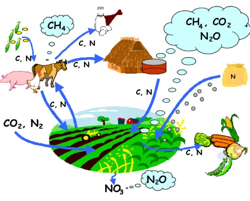
1.2 Greenhouse gas emissions
In agriculture the two major greenhouse gasses are methane (CH4) and nitrous oxide (N2O).
Enteric fermentation by ruminants and emissions from manure management are the two main sources of methane. The main sources of N2O are manure management and soil emissions.
Three sources of N2O soil emissions can be distinguished: 1) direct emissions from fertilizer and
manure application, crop residues and mineralisation of peat soils, 2) emissions from manure and urine during grazing, and 3) indirect emissions due to leaching and runoff of nitrogen. Changes in land use can be a major source of CO2, but also a sink. Figure 1 shows a schematic
overview of the main greenhouse gas emissions sources from agriculture.
Changes in land use have an influence on carbon stocks in the biomass as well as in the soil. Other sources of CO2 are liming of agricultural soils to decrease the acidity and decomposition
of organic soils that are used for agriculture. The total emission of greenhouse gases from agriculture is the sum of CO2, CH4 and N2O, expressed in CO2 equivalents. These are
calculated based on the global warming potentials, which are 1 for CO2, 25 for CH4 and 298 for
Page 12 of 32 WAB 500102 026
CH
4 C, N C, N - -C, N C, NCO
2, N
2 C, N C, N NCH
4, CO
2,
N
2O
NO
3N
2O
CH
4 C, N C, N - -- -- -- ---- ---C, N C, NCO
2, N
2 C, N C, N NCH
4, CO
2,
N
2O
NO
3N
2O
Figure 1. Schematic overview of the main greenhouse gas emissions in agriculture and the relation with the different flows of C and N
1.3 Objective
The objective of this study is to assess the impact of the four Eururalis base scenarios and the CAP options on the emission of greenhouse gasses from agriculture. The results give insight in the emissions of greenhouse gasses in 2030 for the different scenarios and the differences with the current level of GHG emissions at member state and EU level. The results will give an indication of the range of GHG emissions between the four diverging base scenarios and the impact of the policy options regarding the CAP reform.
2 Methodology
2.1 Eururalis
Eururalis is an integrated impact assessment tool which uses four base scenarios to explore future developments of rural areas in Europe within the (dynamic) global context. Results are generated at different aggregation levels, from regions to the whole of Europe and the intermediate aggregation levels. The results facilitate a clear illustration of the trade-offs of policies and world visions as expressed by numerous indicators for European regions and trade-offs over time.
Eururalis is based on a conceptual multi-model framework and has a powerful toolbox with data and scientific models to support interactive use. Models incorporated in the framework are: LEITAP (Van Meijl et al., 2006), IMAGE (Eickhout et al., 2006) and CLUE-s (Verburg et al., 2006). Eururalis is based on four scenarios that are derived from the IPCC SRES scenarios. The time frame used in Eururalis simulations ranges from 2000 to 2030. Data used in the model originate from CPB, UN and FAO. Results and interpretations are presented in maps, graphs, facts, and figures. Eururalis 2.0 results are presented in Rienks (2008) and a detailed description of the Eururalis modelling framework and the presentation tool are provided in Eickhout and Prins (2008).
The approach of using multiple divergent scenarios, distinguishes the Eururalis project from other scenario studies. Four baseline scenarios were elaborated in Eururalis. Within each scenario a different, but consistent, evolution towards 2030 was elaborated. It is possible in each scenario to review similar strategic policy variants. The scenarios represent uncertainties as to how the world might develop, i.e. scenarios are used to indicate what could happen. Such scenarios help to delineate the margins of the possible and conceivable, and are a means to explore and map uncertainties in the development and the impacts of policy options. Eururalis especially focuses on land-use and related issues.
2.2 IMAGE and LEITAP
The combination of LEITAP and IMAGE provides a global context for further European analyses on both economic and ecological aspects at the geographical level of world regions and European member states. LEITAP is a general equilibrium model, based on expected economic growth (GDP), demographic developments and policy changes. LEITAP calculates commodity trade, commodity price and commodity production (actual yield) for each region in the world. Trade barriers, agricultural policies and technological development are taken into account. LEITAP is based on the standard GTAP model
(https://www.gtap.agecon.purdue.edu/models/current.asp). Changes in LEITAP compared to GTAP are documented in Van Meijl et al. (2006). Recent improvements on the land supply curve, biofuels and the consumption function are documented in Eickhout et al. (2007), Banse et al. (2008) and Eickhout et al. (2009) respectively.
IMAGE is an integrated assessment model that simulates greenhouse gas emissions out of the energy system and the land-use system. The land-use system is simulated at a global grid level (0.5 by 0.5 degrees), leading to land-specific CO2 emissions and sequestration and other land
related emissions like CH4 from animals and N2O from fertilizer use (MNP, 2006). IMAGE is
strong in feedbacks by simulating the impacts of CO2 concentrations and climate change on the
agricultural sector and natural biomes (Leemans et al., 2002). Due to these feedbacks impacts of climate change can be assessed (Leemans and Eickhout, 2004). By combining LEITAP and IMAGE (Eickhout et al., 2006) the ecological consequences of changes in agricultural consumption, production and trade can be visualized
The combination of LEITAP and IMAGE captures the effect of global changes on European land use. This global level assessment also allows for evaluating the effects of changes in Europe on
Page 14 of 32 WAB 500102 026
other parts of the world. For instance, trade-offs to environment in developing countries when Europe decides to import biofuels instead of growing them in Europe. LEITAP calculates the economic consequences for the agricultural sector by describing features of the global food market and the dynamics that arise from exogenous scenario assumptions. Regional food production and impacts on productivity (through intensification or extensification) as calculated by LEITAP are used as input of IMAGE. The latter model is used to calculate the effects of land use change and climate change on yield level and simulates feed efficiency rates and a number of environmental indicators (Eickhout et al., 2006). Together, these global models result in an assessment of the agricultural land use changes at the level of individual countries inside Europe and for larger regions outside Europe (Van Meijl et al. 2006). At the same time these models also calculate changes in other sectors of the economy which are indirectly related to land use.
2.3 MITERRA-Europe
MITERRA-Europe is a deterministic and static N cycling model which calculates N emissions on an annual basis, using N emission factors and N leaching fractions. The MITERRA-Europe model was developed to assess the effects and interactions of policies and measures in agriculture on N losses on a regional level in EU-27 (Velthof et al., 2009). MITERRA-Europe is partly based on the existing models CAPRI (Common Agricultural Policy Regionalised Impact; http://www.capri-model.org), and RAINS/GAINS (Greenhouse Gas and Air Pollution Interactions and Synergies; http://gains.iiasa.ac.at/gains/), and was supplemented with an N leaching module, a soil carbon module and a measures module. The input data consists of activity data (from e.g. FAO, Eurostat and JRC) and emission factors. The model includes measures to mitigate NH3 emission and NO3 leaching, and for this study additional measures aimed at the
mitigation of greenhouse gas emissions were added.
The RAINS/GAINS model estimates current and future gaseous N and C emissions from agriculture (and other sectors) in Europe. It incorporates databases on economic activities, e.g. forecast of agricultural activities and number of livestock. Emission factors and removal efficiencies used in RAINS/GAINS are derived from various studies. CAPRI is an agricultural sector model on a regional level in EU-27, with a global market model for agricultural products. Agricultural supply is derived from 38 crops and 19 animal activities covering most agricultural activities. Feed and further input demand are modelled in detail. Major results of the system include yields, cropped areas, number of animals, output quantities, and emissions to the environment and the economic consequences of environmental and economic policies.
The carbon module of MITERRA-Europe (Lesschen et al., 2008) assesses changes in soil organic carbon according to the default IPCC Tier1 approach. Volume 4 of the 2006 IPCC Guidelines for National Greenhouse Gas Inventories (http://www.ipcc-nggip.iges.or.jp/public/2006gl/vol4.html) provides the guidance on the estimation of emissions and removals of CO2 and non-CO2
greenhouse gasses (GHG). In MITERRA-Europe the Tier 1 approach was implemented, since data availability excludes a Tier 2 or 3 approach at EU-27 level.
2.3.1 CH4 emission
The two main sources of methane from agriculture are enteric fermentation by ruminants and emissions from manure management. Methane emissions were calculated with emission factors, which were derived from the IPCC 2006 guidelines. For enteric fermentation an emission factor based on livestock type was used and a distinction was made between Western and Eastern Europe (Table 1). For manure management the emission factors depended on animal type, temperature and manure system and a distinction was made between Western and Eastern Europe (Table 2). Within the model more specific emission factors were used for each country, based on the average annual temperature. These emission factors were in between the values of Table 2. Besides these two main sources of methane, also methane produced during grazing and methane from rice cultivation were taken into account.
Table 1. Emission factors for enteric fermentation (kg CH4 per animal per year)
Livestock type Western Europe Eastern Europe
Dairy cows 109 89
Beef cows 57 58
Pigs 1.5 1
Poultry 0 0
Sheep and goats 7 5
Horses 18 18
Fur animals 0 0
Table 2. Emission factors for manure management (kg CH4 per animal per year)
Livestock type Manure system Western Europe Eastern Europe
Cold Warm Cold Warm Dairy cows Liquid 50.9 86.8 44.9 76.6
Dairy cows Solid 6.0 12.0 5.3 10.6 Beef cows Liquid 19.5 33.2 19.1 32.6 Beef cows Solid 2.3 4.6 2.2 4.5
Pigs Liquid 7.1 12.1 4.4 7.0 Pigs Solid 0.8 1.7 0.9 1.8 Sheep 0.19 0.28 0.10 0.15 Goats 0.13 0.20 0.11 0.17 Horses 1.56 2.34 1.09 1.64 Poultry 0.03 0.03 0.02 0.02 2.3.2 N2O emission
N2O is formed in the soil during the microbiological processes of nitrification and denitrification.
Nitrification concerns the process whereby ammonia under aerobic conditions is converted into nitrate by bacteria. Denitrification is the process whereby, under anaerobic conditions, bacteria convert nitrate into the gaseous nitrogen compounds N2 and N2O. The main sources of N2O are
manure management and emissions from agricultural soils, which can be subdivided in i) direct soil emissions from the application of fertilizers and animal manure, crop residues and the cultivation of Histosols, ii) animal manure produced in the meadow during grazing, and iii) indirect emissions from N leaching and runoff, and from N deposition.
The N2O emission were calculated with N2O emission factors, which were derived from the
IPCC 2006 guidelines (Table 3). For leaching MITERRA-Europe has its own approach and does not use the default IPCC leaching fraction of 30%. The leaching fractions were determined based on texture, land use, precipitation surplus, organic carbon content, temperature and rooting depth. Besides N losses due to leaching also surface runoff was taken into account. These surface runoff fractions were calculated based on slope, land use, precipitation surplus, soil texture and soil depth.
Table 3. N2O emission factors according to IPCC 2006 guidelines
Source Emission factor (%)
Mineral fertilizer 1.0
Applied manure 1.0
Crop residues 1.0
N deposition 1.0
Excretion during grazing for cattle, pigs and poultry 2.0 Excretion during grazing for sheep and other animals 1.0 Indirect emission from leaching and runoff 0.75
Agriculture on organic soils (kg N2O-N ha-1) 8.0 Liquid manure systems (cattle and pigs) 0.1
Solid manure systems (cattle and pigs) 2.0 Manure management (other animals) 0.37 - 0.73
Page 16 of 32 WAB 500102 026
2.3.3 CO2 emission
The IPCC protocol distinguishes six types of land use: forest land, cropland, grassland, wetlands, settlements and other land. In Eururalis the land uses wetland and other land are fixed and do not change over time. For this study we extended these land use types with perennial crops and abandoned land. The protocol distinguishes between two categories: i) no land use change and ii) land use change. Furthermore changes in carbon are calculated for i) a change of carbon in biomass and ii) a change of carbon in soil. In this study we only consider the changes in soil organic carbon and not in biomass, since changes biomass carbon are mainly related to the forest land, while this study focuses on agricultural land. The annual change in soil organic carbon (SOC) stocks is calculated for each land use type as the change in SOC from mineral soils, minus the emissions from organic soils and the emissions due to liming. The amount of soil organic carbon in mineral soils is calculated by multiplying a default reference value, which is a function of soil type and climate, with a coefficient for land use, a coefficient for management and a coefficient for input crop production. Different mitigation options can be modelled with MITERRA-Europe by changing these land use and management factors to assess their effects on soil organic carbon stocks (Lesschen et al. 2008).
The amount of organic carbon of mineral soils (SOC) is calculated as:
SOC = SOCREF * FLU * FMG * FI (1)
with
SOCREF = reference carbon content of the soil (ton C per ha)
FLU = coefficient for land use
FMG = coefficient for management
FI = coefficient for input crop production
SOCREF is the reference carbon stock to a depth of 30 cm, which is a function of soil type and
climate region (Table 4). Thisdata was combined with the data at HSMU-level (soil type and climate region) to calculate an average SOCREF per NUTS2 region. The resulting SOCREF
ranges from 36 to 113 t C ha-1 in the topsoil (0-30 cm). Table 5 shows the assignment of FLU,
FMG and FI to the land use and management types as used in MITERRA-Europe.
Table 4. SOCREF per climate and soil type (ton C ha-1)
Region HAC soils
LAC soils Sandy soils Spodic soils Volcanic soils Wetland soils Boreal 68 NA 10 117 20 146
Cold temperate, dry 50 33 34 115* 20 87 Cold temperate, moist 95 85 71 115 130 87 Warm temperate, dry 38 24 19 80* 70 88 Warm temperate, moist 88 63 34 80* 80 88 * Estimated
Besides changes in SOC due to changes in land use or agricultural management, also CO2
emissions from agriculture on organic soils and liming were taken into account. Agriculture on organic soils leads to loss of carbon due to drainage and tillage, which enhances oxidation of peat. The carbon emissions of organic soils that are used as cropland or managed grassland were related to climate (Table 6). For liming the emission factor is 12% for limestone (CaCO3)
and 13% for dolomite (CaMg(CO3)2), all carbon from liming is thus assumed to be emitted. Data
on liming rates were derived from the national inventories of several EU-15 countries. For Mediterranean countries zero liming was assumed because of their soils with in general high carbonate contents. For the EU-12 countries the average of the EU-15 countries was used.
Table 5. Relative stock change factors for cropland and grassland in MITERRA-Europe Land use and management
types Land use (FLU) Management (FMG) Input (FI)
Intensively managed grassland 1.00 1.14 1.11 Extensively managed grassland 1.00 1.14 1.00 Rough grazing grassland 1.00 1.00 1.00 Long term cultivated 0.80 (dry)
0.69 (wet) Long term perennials 1.00
Paddy Rice 1.10 1.00 1.00
Abandoned land 0.93 (dry) 0.82 (wet)
Full tillage 1.00
Reduced tillage 1.02 (dry) 1.08 (wet)
No tillage 1.10 (dry)
1.15 (wet)
Low input 0.95 (dry)
0.92 (wet)
Medium Input 1.00
High input / no manure 1.04 (dry) 1.11 (wet) High input / with manure 1.37 (dry) 1.44 (wet)
Table 6. Emission factor for organic soils (ton C ha-1 year-1)
Climate Grassland Cropland
Cold 0.25 5
Warm 2.5 10
2.3.4 Mitigation measures
For this study the effect of greenhouse gas mitigation measures was assessed as well. Four types of measures were defined, which increase soil organic carbon (reduced and zero tillage and increased carbon input), decrease N2O emissions (efficient fertilizer use) and decrease CH4
emission (methane reduction). These four measures are described in more detail below. Their implementation within the scenarios is described in Section 2.4.2.
Reduced and zero tillage
Advances in weed control methods and farm machinery allow many crops to be grown without or with reduced tillage. In general, tillage promotes decomposition, reduces soil organic carbon (SOC) stocks and increases emissions of greenhouse gasses through increased aeration, crop residue incorporation into soil, and disruption of aggregates protecting soil organic matter. Therefore reduced or zero tillage often increases SOC. According to the IPCC approach reduced tillage increases SOC with about 5% and zero tillage with about 15% over a period of 20 years. In MITERRA-Europe this measure was implemented by changing the FMG stock
change factor from Full to Reduced or to No.
Increased carbon input
This measure comprises several measures which all provide additional carbon to the soil. One is the inclusion of different crop types in crop rotations, which can increase carbon sequestration. Adding legumes (N-fixing crops such as beans, peas, soya or clover) to rotations of cereals reduces N fertilizer requirements and related emissions, and can increase soil organic carbon as well. Another option is cover or catch crops, which provide a temporary vegetative cover between agricultural crops, which is then ploughed into the soil. These cover crops add carbon to soils and may also extract plant-available N unused by the preceding crop. A final option is crop residue incorporation, where stubble, straw or other crop residues are left
Page 18 of 32 WAB 500102 026
on the field and incorporated into the soil when the field is tilled. However, most of these measures increase the N input, which might lead to increased N2O emissions from crop
residues. In MITERRA-Europe this measure was implemented by changing the FI stock change
factor from Low to Medium or Medium to High.
Efficient fertilizer use
This measure comprises several measures related to fertilizer application and fertilizer type, which increase the fertilizer use efficiency and reduce N2O emissions. Optimising fertilizer
application (e.g. changing fertilizer rates and precision farming) can lead to lower fertilizer application rates and a correct timing of fertilizer application and split applications of N will lower the emission of N2O. The use of other fertilizer types (e.g. nitrification inhibitors or slow release
fertilizers) can also decrease N2O emission. In MITERRA-Europe this measure was
implemented by reducing the fertilizer application by 10%, a reduction of the N2O emission
factor by 15%, and a reduction of the leaching fraction by 10%.
Methane reduction
For reduction of methane emissions several measures exists for the livestock sector. Two types of measures can be distinguished, i) reduction of CH4 from enteric fermentation, e.g. changes in
feed intake or feed additives, and ii) reduction of CH4 emission from manure management, e.g.
manure digestion and adapted stable designs. In MITERRA-Europe these measures were implemented by assuming a 5% reduction of the CH4 emissions from enteric fermentation for
the feeding strategies, and a 50% reduction for the CH4 emission from manure management.
2.4 Scenarios
2.4.1 Scenario descriptions
In Eururalis four base scenarios have been developed, based on the IPCC SRES scenarios, with contrasting narratives of global developments: A1 global economy, A2 continental markets, B1 global co-operation and B2 regional communities (Westhoek et al., 2006). For this study we assessed the GHG emissions for the four base scenarios and for the minimum and maximum CAP variants of the A1 and B2 scenarios (no full liberalisation in A1 and two variations of B2 in which agricultural support is further increased and decreased compared to the baseline in which agricultural support is maintained).
The four contrasting baselines relate to different plausible developments defined by two axes (Nakicenovic, 2000). The two axes relate the way policy approaches problems and long term strategies. The vertical axis represents a global approach as opposed to a more regional approach, whereas the horizontal axis represents market-orientation versus a higher level of governmental intervention. The most important differences between the four scenarios are defined by political developments, macro economic growth, demographic developments and technological assumptions.
The A1 scenario depicts a world with fewer borders and less government intervention compared with today. Trade barriers are removed and there is an open flow of capital, people and goods, leading to a rapid economic growth, of which many (but not all) individuals and countries benefit. There is a strong technological development. The role of the government is very limited. Nature and environmental problems are not seen as a priority of the government. Consequently, border support and income support is phased out in this scenario. Support in Less Favoured Areas (LFA), which compensates farmers in areas with less favoured farming conditions, is also abolished in A1, as it is seen as market distortion
The A2 scenario depicts a world of divided regional blocks. The EU, USA and other OECD countries together form one block. Other blocks are for example Latin America, the former Soviet Union and the Arab world. Each block is striving for self sufficiency, in order to be less reliant on other blocks. Agricultural trade barriers and support mechanisms continue to exist. A
minimum of government intervention is preferred, resulting in loosely interpreted directives and regulations. In A2, the income and border support is maintained, as is LFA policies.
The B1 scenario depicts a world of successful international cooperation, aimed at reducing poverty and reducing environmental problems. Trade barriers will be removed. Many aspects will be regulated by the government, e.g. carbon dioxide emissions, food safety and biodiversity. The maintenance of cultural and natural heritage is mainly publicly funded. Therefore, income support is reduced to 33% and is shifted to maintain environmental services. Border support is phased out as well, as this is seen as unfair to developing countries. In B1 LFA is maintained, except for arable agriculture in locations with high erosion risk.
The B2 scenario depicts a world of regions. People have a strong focus on their local and regional community and prefer locally produced food. Agricultural policy is aiming at self sufficiency. Ecological stewardship is very important. This world is strongly regulated by government interventions, resulting in restrictive rules in spatial policy and incentives to keep small scale agriculture. Economic growth in this scenario is the lowest of all four. In B2, agri-environmental payments are raised with 10% and LFA is maintained, although arable areas prone to high erosion risk are excluded. Border support is maintained to stimulate self-sufficiency of the EU, although export subsidies are abolished.
The CAP variant of the A1 scenario is not abolishing income support but is only decreasing it. Consequently, the budget for income support will be reduced by 50% in 2030. This variation is limited, but further de-liberalisation is regarded very unlikely in a world that is as market oriented as the A1 scenario. The variations on B2 work in two directions: one variant provides more liberalisation by reducing market price support after 2020 by 50% and one variant is even increasing income support by increasing the budget for income support with 50% in 2030. We calculated GHG emissions for 2000, 2010, 2020 and 2030, which were also the periods for which IMAGE-LEITAP makes its simulations. In MITERRA-Europe the following variables changed for the different scenarios and the different simulation years:
• Crop areas (relative changes derived from CLUE-s results) • Number of animals (relative changes derived from IMAGE results) • Crop yield (relative changes derived from IMAGE results)
• Fertilizer application (relative changes derived from IMAGE results) • NH3 emission control strategies (derived from RAINS-GAINS scenarios)
• Implementation of measures (see section 2.4.2)
Land use change, which is the main driver for changes in soil organic carbon, is calculated from the CLUE-s results, as the average change during the previous 10 years, e.g. for 2010 the change is calculated for the period 2000-2010. However, for the year 2000 no land use change is taken into account, since no consistent data for the period 1990-2000 was available. Therefore the CO2 emissions from land use change in mineral soils were not calculated for
2000.
2.4.2 Measures within the scenarios
Table 7 presents a summary of the most important characteristics of the four base scenarios, in relation to GHG mitigation measures.
Table 7. Summary of the most important characteristics of the four Eururalis scenarios for the definition of greenhouse gas mitigation measures (based on Eickhout and Prins (2008))
Environmental policy Agro-technology Erosion policy Bioenergy N-use efficiency
A1 No High No No target 10%
A2 No Low No No target 10%
B1 Yes High Yes Target 25%
Page 20 of 32 WAB 500102 026
The degree of implementation of the mitigation measures varies for the different Eururalis scenarios and has been qualitatively defined in Table 8. In scenario A1 (global economy) there is no environmental policy, but agro-technology is high, which stimulates the measures efficient fertilizer use and methane reduction. Scenario A2 (continental markets) assumes no implementation of mitigation measures at all, due to lack of environmental policy and low agro-technology. For scenario B1 (global co-operation) successful climate mitigation strategies are assumed, by putting a price on carbon. This will lead to large-scale implementation of GHG mitigation measures. However, the stimulation of bioenergy will result in increased use of crop residues, which will lower the input of carbon to the soil. Therefore the positive effect cover crops and crop rotations, as stimulated by the environmental and erosion policies, are partly counterbalanced by the increased demand for bioenergy. Finally, in the B2 scenario (regional communities) mitigation measures are stimulated, but methane reduction is less achieved compared to B1, since this measure requires a high level of agro-technology.
Table 8. Implementation of mitigation measures for the four Eururalis scenarios
Reduced tillage Increased C input Efficient fertilizer use CH4 reduction
A1 + 0 + +
A2 0 0 0 0
B1 ++ + ++ ++
B2 ++ + + +
Based on Table 7 the degree of implementation of the four measures was estimated for each scenario and for the years 2000, 2010, 2020 and 2030 (Table 9). A further distinction was made between the EU15 and EU12 countries, to account for their recent joining to the European Union, which allows them more time to reach EU targets and to comply with EU policies. The degree of implementation for the base year was partly based on Velthof et al. (2007) and Lesschen et al. (2008).
Table 9. Degree of implementation of the four measures, for the EU15 and EU12 and for the four scenarios and different years
2000 2010 2020 2030 EU15 EU12 EU15 EU12 EU15 EU12 EU15 EU12 Reduced tillage A1 15 10 20 15 30 25 35 35 A2 15 10 15 10 15 10 15 10 B1 15 10 30 25 50 50 50 50 B2 15 10 30 25 50 50 50 50 Increased C input A1 30 25 30 25 30 30 30 30 A2 30 25 30 25 30 30 30 30 B1 30 25 45 40 60 55 60 60 B2 30 25 45 40 60 55 60 60 Efficient fertilizer use A1 50 25 55 30 60 40 70 50 A2 50 25 45 25 40 20 40 20 B1 50 25 70 50 90 70 90 70 B2 50 25 55 35 60 50 70 60 Methane reduction A1 0 0 10 5 30 20 30 20 A2 0 0 0 0 0 0 0 0 B1 0 0 10 5 30 25 70 60 B2 0 0 5 0 15 10 30 25
3
Results and discussion
3.1 European results
3.1.1 Total GHG emissions
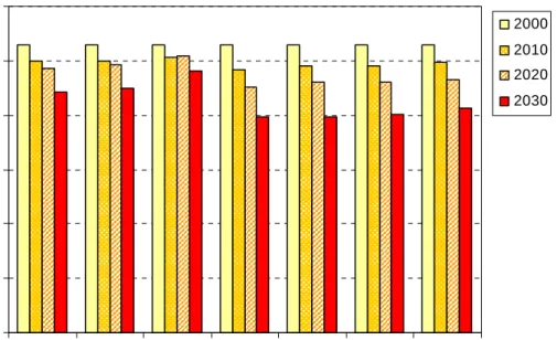
Figure 2 shows the GHG emissions from agriculture for the different scenarios and different years. For 2000 the GHG emission from agriculture was 529 Mton CO2-equivalent, whereas in
2030 the lowest projected emissions were 397 Mton CO2-equivalent for the B1 scenario. In all
scenarios emissions decreased with time, however the rate of decrease varied between the scenarios. In the B1 and B2 scenario the reduction of GHG emission was stronger than in the A1 and A2 scenario. The effect of the CAP options was only minor compared to the emissions over time and for the different scenarios. The CAP options showed that GHG emissions are higher with less liberalisation and more income support.
0 100 200 300 400 500 600 A1 A1 less lib. A2 B1 B2 more lib. B2 B2 more support G H G e m is s ion ( M ton C O 2 -e q /y e a r) 2000 2010 2020 2030
Figure 2. Development of total GHG emissions from agriculture for the different scenarios in the EU-27
To explain the differences between the scenarios it is necessary to have insight into the main drivers for the GHG emissions. Although there are many factors changing between the scenarios and over time, the main drivers are crop areas (land use) and livestock numbers. Figure 3 shows the development of the agricultural area for the EU-27 for the different scenarios. For 2000 the agricultural area is derived from the crop areas from CAPRI, and for the other years the area is multiplied with the relative changes in agricultural land as obtained from the CLUE results. In all scenarios the agricultural area is decreasing in Europe, only in the A2 scenario it stabilises after 2010. This pattern is also found in the emissions, since less agricultural land means lower N2O soil emissions and increased soil carbon sequestration. One
remark should be made for the decrease between 2000 and 2010. The CORINE land cover map, which is the starting point for 2000, does not consider abandoned land, whereas this is later introduced in the CLUE results, therefore the large decrease in agricultural area between 2000 and 2010 is partly artificial.
WAB 500102 026 Page 22 of 32 0 20 40 60 80 100 120 140 160 180 200 A1 A1 less lib. A2 B1 B2 more lib. B2 B2 more support A g ri c u lt u ra l a re a ( m illio n h a ) 2000 2010 2020 2030
Figure 3. Change in agricultural area for the different scenarios
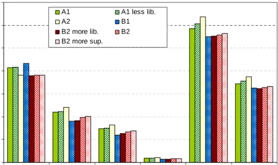
Figure 4 shows the number of livestock for the EU-27 for the different scenarios and livestock categories. In the A2 scenario the number of beef cows, pigs and poultry (meat production) is higher, whereas dairy farming is more important in the A1 and B1 scenario. The number of livestock increases for the CAP options with less liberalisation and more income support. This also explains the increase in GHG emission for these scenarios.
0 10 20 30 40 50 60 70
Dairy cows Beef cows Sheep Goats Pigs Poultry
L ivest o c k u n it s ( m illio n L U ) A1 A1 less lib. A2 B1 B2 more lib. B2 B2 more sup.
Figure 4. Number of livestock units for the different scenarios in 2030 (based on IMAGE data)
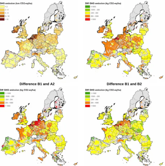
The spatial distribution of GHG emissions over Europe in 2030 is shown in Figure 5 for the B1 scenario. Additionally, the difference in GHG emissions between the B1 scenario the other scenarios is shown. This presentation was chosen since the patterns of the GHG emissions of the four scenarios are rather similar, since differences are relatively small compared to the total
emissions. High emissions occur in regions with high livestock densities, e.g. The Netherlands, Flanders, southern Ireland, but also Estonia has a rather high emission, due to the use of peat soils for agriculture.
B1 Difference B1 and A1
Difference B1 and A2 Difference B1 and B2
Figure 5. Spatial distribution of GHG emissions from agriculture in 2030 (the results were calculated at NUTS2 level, but an overlay was made with the agricultural areas from the CORINE land cover map of 2000)
The comparison with the other scenarios was done for the B1 scenario, since this scenario is generally considered to be closest to the present day reality. Although the B1 scenario has the lowest total emissions (Figure 2), there are still regions that have lower emissions in the other scenarios, e.g. in Portugal and Spain. The A2 scenario, which has the highest emissions, shows that these are mainly caused by higher GHG emissions in Germany, Finland, Belgium and The Netherlands. The B2 scenario, with similar total emissions, has higher GHG emissions in the EU15 countries, i.e. agriculture remains more intensive, and lower emissions in Eastern Europe, i.e. agriculture is more extensive compared to the B1 scenario.
WAB 500102 026 Page 24 of 32
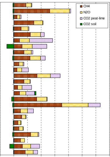
3.1.2 GHG emissions per source
Figure 6 shows the per hectare GHG emissions for each country differentiated for the emission sources. Distinction is made between CH4 (mainly from enteric fermentation by ruminants and
emissions from manure management), N2O (mainly from manure management and direct and
indirect soil emissions), CO2 from the use of peat soils for agriculture and liming, and CO2 from
changes in soil carbon stocks. The figure shows that the emission profiles differ greatly between countries. The highest emissions occur in countries with intensive agriculture on a small area, e.g. The Netherlands and Belgium.
-2 0 2 4 6 8 10 12 14 United Kingdom Sweden Spain Slovenia Slovakia Romania Portugal Poland Netherlands Luxembourg Lithuania Latvia Italy Ireland Hungary Greece Germany France Finland Estonia Denmark Czech Republic Cyprus Bulgaria Belgium Austria
GHG emission (ton CO2-eq/ha)
CH4 N2O
CO2 peat-lime CO2 soil
Figure 6. Sources of GHG emissions per country for the 2010 B1 scenario
CH4 and N2O are for most countries the main GHG sources. The emissions are, on a per
hectare base, high for countries with high livestock densities, e.g. The Netherlands, Belgium and Ireland. CO2 from peat soils and liming is a particularly large source of GHG emissions for
northern European countries, e.g. Finland, Sweden, Estonia and The Netherlands. In addition to the occurrence of peat soils, most soils are acid and liming is therefore a common practice as well in these countries. CO2 from changes in soil carbon stocks is for most countries a sink,
especially Finland and Sweden have large sinks due to agricultural land abandonment. For some countries, e.g. Lithuania, CO2 from changes in carbon soil stocks is a source, due to
conversion to arable land.
Table 10 shows the emissions for the different scenarios and periods for the EU-27, but differentiated to GHG sources. CH4 emissions gradually decreased over time, but for N2O the
main reduction occurred in the period 2020-2030. The emissions from CO2 from SOC stock
changes are mainly negative, which means that carbon is sequestered in the soil. Soil carbon sequestration is higher in the B1 and B2 scenario as a result of higher implementation of mitigation measures. The changes in SOC stocks are also time-dependent, sequestration is higher for 2010 and 2020, since most land use changes occurred during these periods and also the mitigation measures ‘reduced and zero tillage’ and ‘increased C input’ are implemented mainly during these periods.
Table 10. GHG emissions from agriculture in the EU-27 for 2010 (in Mton CO2-eq)
CH4 N2O CO2 emission SOC stocks Total GHG
2000 269 178 82 0.0 529 2010 A1 250 185 77 -11.2 500 A1 less lib. 252 185 75 -11.4 500 A2 254 178 78 -3.2 507 B1 247 174 79 -16.4 484 B2 more lib. 250 176 79 -14.2 491 B2 250 176 78 -13.9 490 B2 more support 254 178 80 -14.6 497 2020 A1 234 186 75 -7.8 486 A1 less lib. 236 186 74 -3.7 493 A2 247 183 79 0.3 510 B1 223 171 75 -18.2 451 B2 more lib. 227 173 76 -15.7 460 B2 227 173 75 -15.0 460 B2 more support 229 175 77 -15.1 466 2030 A1 221 154 72 -5.3 442 A1 less lib. 224 154 72 -2.1 449 A2 238 159 80 4.1 481 B1 191 138 71 -3.1 397 B2 more lib. 195 137 72 -5.6 398 B2 202 139 71 -8.8 403 B2 more support 204 142 74 -7.8 412
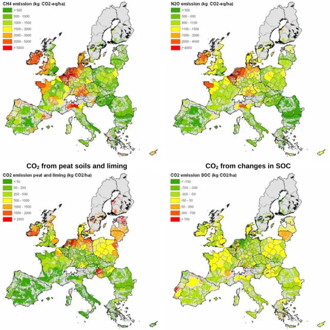
Figure 7 shows the spatial distribution of the GHG emissions from the different sources. For CH4 and N2O the pattern is more or less similar, with high emissions in the livestock intensive
regions, i.e. The Netherlands, Belgium, NW and southern Germany, Ireland, Bretagne and the Po region. CO2 emissions from peat soils and liming are high for regions in northern Europe
with peat soils and a region in Hungary. The CO2 emission from SOC stock changes is more
diverse. In most areas stocks remain equal or slightly increase due to implementation of the mitigation measures and agricultural land abandonment over the period 2000-2010. However, in some regions carbon is lost from the soil due to land conversion for agricultural expansion, e.g. Lithuania and Portugal.
WAB 500102 026 Page 26 of 32
CH4 N2O
CO2 from peat soils and liming CO2 from changes in SOC
Figure 7. Spatial distribution of the different greenhouse gas emissions over Europe. The results of the B1 scenario for 2010 are depicted.
3.1.3 Effect of measures
The previous results for the scenarios are all based on many changing factors, i.e. livestock numbers, crop areas, yield, fertilizer input and mitigation measures. Therefore, we did another analysis to assess the effect of mitigation measures separately. For the A1 and B2 scenario other simulations for 2030 were done with the same settings, except different implementation degrees of the mitigation measures. We used the settings of the A2 (lowest implementation degree) and B1 (highest implementation degree). In addition, two simulations were done for the A1 scenario with zero and full implementation of measures. Table 11 shows that the range in total GHG emission between the measures settings from the A2 and B1 scenario is about 30 (for A1) to 37 (for B2) Mton CO2 equivalents. These differences were much larger compared to
the effect of the different CAP options (Table 10). The results for the simulation with zero and full implementation showed an even larger difference (127 Mton CO2 equivalents). This is about
a quarter of the current GHG emissions from agriculture. For CH4 a reduction of 37 Mton CO2
67 Mton CO2-eq could be possible compared to the situation without measures. However, for
the last category should be noted that this reduction is only possible for 20 years (we assumed no implementation in 2020 and full in 2030), whereas the emission reduction for CH4 and N2O
can be obtained every year.
Table 11. Influence of measures versus CAP on the GHG emissions for the year 2030 (in Mton CO2-eq)
Scenario Measures CH4 N2O
CO2
peat+lime CO2 change SOC Total GHG A1 A1 220.5 154.3 72.0 -5.3 441.5 A2 231.2 160.8 72.0 0.0 460.6 B1 205.6 149.6 72.0 -3.2 424.0 No measures 231.2 168.8 72.0 -3.8 468.1 Full implementation 193.8 146.0 72.0 -71.1 340.7 B2 B2 201.6 138.6 71.3 -8.8 402.7 A2 211.8 143.0 71.3 -9.6 416.4 B1 187.9 136.6 71.3 -8.8 387.0
3.1.4 Differences between IPCC guidelines
For this study we used emission factors and calculation rules according to the most recent IPCC guidelines, i.e. from 2006. However, for the reporting to the UNFCCC member states still report their emissions according to the IPCC guidelines of 1996 or national methodologies. In the guidelines of 1996 the N2O emission factor for N input was higher (1.25 versus 1.00), the CH4
emission from enteric fermentation was lower, especially for cows, the CH4 emission factor for
manure storage was on average lower and the emission factor for cropland on peat soils was lower for cold areas (1.0 versus 5.0 ton C/ha). These changes explain the main differences in outcome between the two guidelines, i.e. lower CH4 emission, higher N2O emission and lower
CO2 emission from peat soils according to the IPCC 1996 guidelines (Table 12).
Table 12. GHG emissions from agriculture, calculated according to IPCC 2006 and 1996 guidelines for the A1 scenario in 2030 (in Mton CO2-eq)
Emissions IPCC 2006 guidelines IPCC 1996 guidelines
CH4 emission 221 202
N2O emission 154 176
CO2 from peat soils and liming 72 37 CO2 from change in SOC -5.3 -7.4 Total GHG emissions 442 408
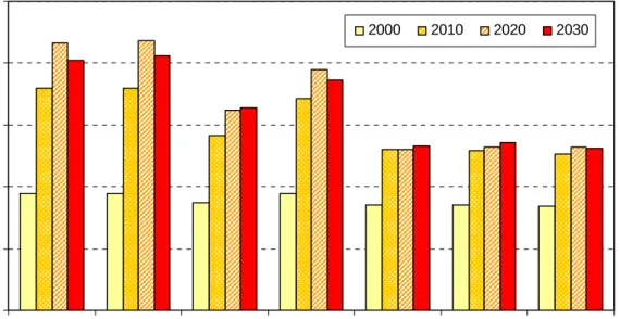
3.2 Global results
Globally, land use related GHG emissions are increasing in all scenarios until 2030. Figure 8 shows the absolute amount of land use related emissions. A major source of land use related GHG emissions is the conversion of nature to agricultural land. The amount of conversion depends on economic developments, population growth, technology, and policy measures. In an open world, i.e. Global economy (A1) and Global Cooperation (B1), economic growth and medium population dynamics cause the highest agricultural demand. Although technological development, and thus crop yields increase, the global agricultural area is expanding by more than 20%. Therefore change in land use related GHG emissions range from an increase of 56% (B2) to an increase of 114% (A1) between the four scenarios.
WAB 500102 026 Page 28 of 32 0 5 10 15 20 25
A1 A1 less lib. A2 B1 B2 B2 more lib. B2 more support G H G em is s io n ( G to n C O 2-eq /year ) 2000 2010 2020 2030
Figure 8. Global greenhouse gas emissions (in Gton CO2-eq per year)
Another important driver, especially for land use related emissions, is the developments of agricultural (trade) policies. In which region is the production of agricultural commodities expected? And is expansion of agricultural area needed or can the commodities be produced at the current agricultural area. Table 13 gives an insight in the agricultural expansion for the different world regions. The A2 scenario depicts a world of divided regional blocks and therefore trade policies between North America and Europe on the one hand and Latin America on the other hand are not very liberal. This results in an expansion of agriculture in North America and a stabilisation in Europe. The area in Latin America is expanding by 8%, which is small compared to the 31% to 42% increase in the B1 and A1 scenarios respectively. Other regions expand less or even decrease their agricultural area in the A2 scenario. Beside the agricultural policies, lower economic growth (e.g. in Sub-Saharan Africa) also accounts for a smaller agricultural area. Global expansion of agricultural area in A2 is only 60% of the expansion in the A1 (the expansion in A2 is 14%, whereas the expansion in A1 is 24%). Cumulative land related GHG emissions from 2000 to 2030 on the other hand, are only 21% lower in the A2 scenario compared to the A1 scenario. So, with regard to emissions, the use of existing agricultural area instead of expansion is more efficient and does lower the GHG emissions per hectare expanded area.
Table 13. Developments in agricultural area in world regions
World region 2000 2000-2030 A1 A1 less lib. A2 B1 B2 B2 more lib. B2 more support million km2 % % % % % % % North America 5.8 6 11 20 0 2 2 5 Latin America 6.7 42 42 8 31 9 13 8 Middle East and North Africa 2.8 4 3 1 4 2 2 2 Sub-Saharan Africa 10.1 60 60 45 61 24 23 23 Former Soviet Union 5.5 13 12 -9 8 -17 -17 -17
Europe 2.2 -7 -3 1 -13 -13 -15 -12
Asia 10.6 11 11 7 4 6 6 6
Oceania 4.8 12 11 3 8 -3 -2 -3
The increase in emissions form industry and energy depends on the scenario and the implemented policies. Differences in management practices in land use are not taken into account in the IMAGE model. Land use related emissions count for one third in the B1 scenario, where the increase in other emissions is successfully tackled, whereas in the other scenarios land use emissions count for one fourth of total emissions. The land use related emissions do matter at the global scale. If other sectors do decrease their emissions or emission factors, it will be increasingly important to decrease the land use emissions too.
Changes in income subsidy in the Common Agricultural Policies hardly had an impact on land use in other regions. The reason for the increase in agricultural land use in the A1 less liberalisation scenario in North America was the increases in income subsidies. The B2 world depicts a world with regionalization (e.g. preference for regional products). Due to this trend, the
more liberalisation option did only have a small effect on land use change within this scenario.
In Brazil agricultural expansion was higher, whereas the agricultural area in Europe was decreasing more. Impacts of changes in European agricultural policies on land use related emissions were small (Figure 8).
WAB 500102 026 Page 30 of 32
4 Conclusions
GHG emissions incl. SOC stock changes from agriculture in the EU-27 were 529 Mton CO2
-equivalents in 2000, which is about 13% of the total GHG emission in Europe. The projected GHG emissions from agriculture are decreasing in all scenarios, ranging between 397 Mton CO2-equivalents for the B1 scenario to 482 Mton CO2-equivalents for the A2 scenario. The
effect of the CAP options is only minor and shows that GHG emissions are higher with less liberalisation and more income support.
At global scale, the CAP options hardly play a role in total GHG emissions from land use. Much more important are developments in population, economic growth, policies and technological developments as depicted by the different scenarios. Trade policies that favour liberalisation, and therefore shifts in agricultural land use to other regions, e.g. from Europe to Latin America, do cause higher GHG emission per hectare expanded area than less liberalized trade policies. CH4 and N2O are for most countries the main GHG emission sources. These emissions are, on
a per hectare base, particularly high for countries with high livestock densities. CO2 from peat
soils and liming is a particularly large source for northern European countries. CO2 from
changes in soil carbon stocks is for most countries a net sink, however, for some countries where agriculture is expanding the changes in SOC stocks are a net source of CO2.
The analysis of the measures shows that the effect of mitigation measures on GHG emissions is much larger than the effect of the CAP options. Full implementation of the simulated mitigation measures could lead to a reduction of GHG emissions from agriculture by 127 Mton CO2
equivalents, which is about a quarter of the current GHG emissions from agriculture. Promoting mitigation measures is therefore more effective than changes in income and price subsidies within the CAP to reduce GHG emissions from agriculture.
References
Banse, M., Van Meijl, H., Tabeau, A., Woltjer, G., 2008. Will EU biofuel policies affect global agricultural markets? European Review of Agricultural Economics, 35(2): 117-141.
EEA, 2009. Annual European Community greenhouse gas inventory 1990–2007 and inventory report 2009. European Environmental Agency. Technical Report 4/2009.
Eickhout, B., Van Meijl, H., Tabeau, A., 2006. Modelling agricultural trade and food production under different trade policies. In: MNP (2006) (Edited by A.F. Bouwman, T. Kram and K. Klein Goldewijk), Integrated modeling of global environmental change. An overview of IMAGE 2.4. Netherlands Environmental Assessment Agency (MNP), Bilthoven, The Netherlands.
Eickhout, B., Van Meijl, H., Tabeau, A., Van Rheenen, T., 2007. Economic and ecological consequences of four European land-use scenarios. Land Use Policy, 24: 562-575. Eickhout, B., Prins, A.G. (Eds.), 2008. Eururalis 2.0 Technical background and indicator
documentation. Wageningen UR and Netherlands Environmental Assessment Agency (MNP), Wageningen and Bilthoven, The Netherlands.
Eickhout, B., Van Meijl, H., Tabeau, A., Stehfest, E., 2009. The impact of environmental and climate constraints on global food supply. In: “Economic Analysis of Land Use in Global Climate Change Policy”, edited by T. Hertel, S. Rose and R. Tol, Routledge, USA.
Leemans, R., Eickhout, B., 2004. Another reason for concern: regional and global impacts on ecosystems for different levels of climate change. Global Environmental Change, 14: 219-228.
Leemans, R., Eickhout, B., Strengers, B., Bouwman, L., Schaeffer, M., 2002. The consequences of uncertainties in land use, climate and vegetation responses on the terrestrial carbon. Science in China, 45: 126-141.
Lesschen, J.P., Schils, R., Kuikman, P., Oudendag, D., 2008. PICCMAT: implementation of measures to mitigate CO2 and N2O from agricultural systems across EU-27. PICCMAT
Deliverable D7.
MNP, 2006. Integrated modeling of global environmental change. An overview of IMAGE 2.4. Edited by A.F. Bouwman, T. Kram and K. Klein Goldewijk. Netherlands Environmental Assessment Agency (MNP), Bilthoven, The Netherlands.
Nakicenovic (ed.), 2000. Special Report on Emission Scenarios. Intergovernmental Panel on Climate Change (IPCC), Geneva, Switzerland.
Rienks, W.A. (ed.), 2008. The future of rural Europe. An anthology based on the results of the Eururalis 2.0 scenario study. Wageningen UR and Netherlands Environmental Assessment Agency (MNP). Wageningen and Bilthoven, The Netherlands.
Van Meijl, H., van Rheenen, T., Tabeau, A., Eickhout, B., 2006. The impact of different policy environments on land use in Europe. Agriculture, Ecosystems and Environment, 114: 21-38.
Velthof, G.L., Oudendag, D.A., Oenema, O., 2007. Development and application of the integrated nitrogen model MITERRA-Europe. Alterra, Wageningen, The Netherlands. Velthof, G.L., Oudendag, D., Witzke, H.P., Asman, W.A.H., Klimont, Z., Oenema, O. 2009.
Integrated assessment of nitrogen emissions from agriculture in EU-27 using MITERRA-Europe. Journal of Environmental Quality, 38: 402-417.
Verburg, P.H., Schulp, C.J.E., Witte, N., Veldkamp, A., 2006. Downscaling of land use change scenarios to assess the dynamics of European landscapes. Agriculture, Ecosystems & Environment, 114: 39-56.
Westhoek, H.J., van den Berg, M., Bakkes, J.A., 2006. Scenario development to explore the future of Europe's rural areas. Agriculture, Ecosystems & Environment 114, 7-20.