3D packing for optimizing shipping of goods with release and due dates

(1)

3D PACKING FOR OPTIMIZING

SHIPPING OF GOODS WITH RELEASE

AND DUE DATES

Aantal woorden / Word count: 8,090

Taike Ackaert

Stamnummer / student number : 01502965

Promotor / supervisor: Prof. Dr. Veronique Limère

Co-promotor / co-supervisor: Nico Schmid

Masterproef voorgedragen tot het bekomen van de graad van:

Master’s Dissertation submitted to obtain the degree of:

Master in Business Engineering: Operations Management

(2)

(3)

Confidentially agreement

Permission

I declare that the content of this Master’s Dissertation may be consulted and/or reproduced, provided that the source is referenced.

Name student : Taike Ackaert

Signature: Taike Ackaert - August 11, 2020 ii

(4)

(5)

Preface

Under the credo ‘Dare to Think’ of Ghent University, I decided to challenge myself when selecting the subject of my master dissertation. Although the topic of this dissertation inter-ested me immediately, I doubted whether I had the right capabilities to properly complete the research. The making of this dissertation was a great learning process and I am very proud of the obtained result.

The realization of this work would not have been possible without the support of certain people. First, I would like to thank Prof. Dr. V. Lim`ere for giving me the opportunity to dive into this topic as a master dissertation. Also, I would like to thank N. Schmid who has guided me intensively over the past year in order to achieve a good end result. Furthermore, I would like to thank my family and friends for their support, patience, and understanding not only during this intensive period, but during all years of my journey at Ghent University.

(6)

(7)

Abstract

In this dissertation, a multi-container loading problem is presented with a focus on the timing aspect related to the items that need to be loaded into the containers. Both the release time of the items to the shelter space and their due date to obtain on-time delivery are taken into account. Furthermore, special attention was paid to the positioning of the items in the container. In the introduced mathematical model, the positioning of the items is included by means of linear constraints. The complete container loading problem is approached by the construction of an integer linear programming (ILP) model.

The model was tested on two datasets. More specifically, seven scenarios per dataset were analyzed. For each scenario, one parameter value was changed to observe its impact on the solution of the model. Since an optimal solution could not be found after three hours of computation time, additional datasets were analyzed to identify which aspects increase the complexity of solving the model.

(8)

(9)

List of Abbreviations

3D three-dimensional.

CN container number.

DD due date.

DVs decision variables.

ILP integer linear programming. IN item number.

MIKP multiple identical knapsack problem. MILP mixed integer linear programming.

ON order number. OT order time. PN position number. RT release time. VC volume capacity. WC weight capacity. vii

(12)

(13)

List of Figures

3.1 Process description . . . 10

4.1 2x2x2 model representation . . . 16

4.2 2x2x2 representation of rows, columns, and layers . . . 16

4.3 Example of the definition of binary variable cpqk . . . 20

4.4 Example of the definition of binary variable rpqk . . . 21

4.5 Example of the definition of binary variable lpqk . . . 21

5.1 Time lapse of computation scenario 1 dataset 1 . . . 30

5.2 Time lapse of computation scenario 1 dataset 2 . . . 31

5.3 Objective function value per scenario for dataset 1 . . . 32

5.4 Objective function value per scenario for dataset 2 . . . 32

5.5 Timing of items shipped for dataset 1 . . . 34

5.6 Timing of items shipped for dataset 2 . . . 34

5.7 Positioning of items of scenario 1 for dataset 1 . . . 36

5.8 Positioning of items of scenario 1 for dataset 2 . . . 36

(14)

(15)

List of Tables

2.1 Categorization of practical constraints according to Bortfeldt & W¨ascher (2013) 3

4.1 Overview of the sets, parameters, and decision variables . . . 13

4.2 Overview of the binary variables cpqk, rpqk, and lpqk created for the 2x2x2 model 19 5.1 Overview of the content of the datasets . . . 28

5.2 Overview of the different scenarios tested . . . 29

5.3 Solution gap per scenario for dataset 1 and dataset 2 . . . 30

5.4 Overview of the solution gap per scenario for each dataset . . . 37

1 Container data of dataset 1 . . . 45

2 Position data of dataset 1 . . . 45

3 Order data of dataset 1 . . . 46

4 Item data of dataset 1 . . . 47

7 Order data of dataset 2 . . . 49

8 Item data of dataset 2 . . . 50

9 Overview decision variables dataset 1 scenario 1 . . . 51

15 Overview decision variables dataset 1 scenario 7 . . . 57 ix

(16)

List of Tables x

16 Items not loaded per scenario for dataset 1 . . . 57

24 Items not loaded per scenario for dataset 2 . . . 64

25 Objective function values per scenario for dataset 1 . . . 65

26 Objective function values per scenario for dataset 2 . . . 65

27 Overview of early, on-time, late, and non-deliveries for dataset 1 . . . 66

28 Overview of early, on-time, late, and non-deliveries for dataset 2 . . . 66

29 Container data of dataset 3 and dataset 5 . . . 67

31 Position data of dataset 3 and dataset 5 . . . 67

33 Order data of dataset 3 and dataset 4 . . . 69

34 Order data for dataset 5 . . . 70

(17)

(18)

Chapter 1

Introduction

As explained by Bortfeldt & W¨ascher (2013), container loading problems consist of loading cargo, three-dimensional (3D) small items, into 3D, cubic, large containers while satisfying a number of constraints such that a given objective function is optimized. In recent years, container loading problems are widely studied because of their contribution to a more effi-cient operation of companies. Bad container loading might lead to an increase in costs or to a decrease in customer service. However, the complexity of the problem restricts researchers to only consider a limited number of practical constraints in their models in order to achieve optimal solutions.

The studied problem can be categorized as a multiple identical knapsack problem (MIKP), which is an output maximization problem. The MIKP consists in loading a set of identical containers with a selection from heterogeneous items so that the value of the items that are loaded is maximized. The categorization of the proposed model as a MIKP might be some-what confusing given that the objective function of the proposed model minimizes the total cost. However, the number of containers available for loading at each time period is restricted to the number of gates available at the loading place.

In this study, the MIKP is solved by means of an integer linear programming (ILP) model. These models are flexible in adding and removing constraints to meet the conditions in spe-cific problem cases. Moreover, ILP models are relatively easy to implement and the currently available solvers have a good computational performance. For single container loading prob-lems, ILP models have been commonly used (Junqueira et al. (2012), Huang et al. (2016))

(19)

Chapter 1. Introduction 2

while results for multi-container problems are still rather limited.

The container loading literature already includes a wide variety of practical constraints re-lated to the weight of containers (Davies & Bischoff (1999)), the weight distribution of items inside a container (Ramos et al. (2018)), the arrangement of boxes in a container (Junqueira et al. (2012), Alonso et al. (2019)), etc. However, for the construction of the container loading problems, it is commonly assumed that the boxes to be loaded in the container(s) are always available for loading.

The focus of this master dissertation is on loading items in a container so that they are deliv-ered to the customer on time. To be useful in practice, the release times of the items to the shelter space and the time needed to load items in a container must be taken into account. The assumption is made that sufficient containers of identical size are available to fulfill all the orders. However, not all containers can be loaded at the same time since companies are limited in the number of gates available to load the containers. Furthermore, the positioning of the ordered items into the containers are included as linear constraints in the mathemat-ical model. While there are many heuristic approaches to packing boxes into the container (Pisinger (2002)), much less exact algorithms have been proposed (Martello et al. (2000)).

The structure of this paper is as follows. First, a short literature review on container loading problems is presented, more specifically with a focus on practical constraints that are added to basic models. In the next chapter, the overall process of the research topic is briefly explained. Thereafter, the mathematical model is presented, followed by the chapter that embodies the datasets on which the model has been tested and their obtained results. This chapter also addresses the limitations of this study. Finally, the conclusions are drawn.

(20)

Chapter 2

Literature study

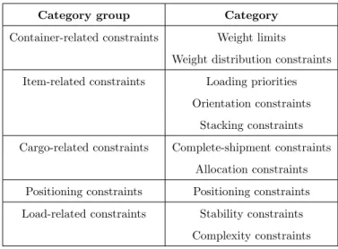
In recent years, practical constraints have received increasing attention in the research domain of container loading problems. Bischoff & Ratcliff (1995) summed up twelve considerations to be taken into account for the construction of feasible container loading plans. Later, Bortfeldt & W¨ascher (2013) published a complete review of the container loading problem and its practical constraints. These constraints were categorized as represented in table 2.1.

Category group Category

Container-related constraints Weight limits

Weight distribution constraints

Item-related constraints Loading priorities

Orientation constraints Stacking constraints

Cargo-related constraints Complete-shipment constraints

Allocation constraints

Positioning constraints Positioning constraints

Load-related constraints Stability constraints

Complexity constraints

Table 2.1: Categorization of practical constraints according to Bortfeldt & W¨ascher (2013)

(21)

Chapter 2. Literature study 4

The terminology as proposed by Bortfeldt & W¨ascher (2013) is often used as a reference framework in literature. According to this framework, two types of container loading prob-lems can be distinguished. Input value minimization probprob-lems assume sufficient containers to be available to accommodate all small items while output value maximization problems assume a limited availability of containers such that only a subset of the cargo can be loaded. While the review of Bortfeldt & W¨ascher (2013) focuses on constraints, the review of Zhao et al. (2016) instead emphasizes the description of algorithms available to solve container loading problems.

Widely discussed are the practical constraints related to weight. Weight capacity constraints ensure that the maximum permitted container weight cannot be exceeded (Liu & Chen (1981)). Furthermore, there are constraints limiting the weight that each axle of a truck can bear (Alonso et al. (2017)). Moreover, constraints concerning the weight distribution of the cargo are considered (Bortfeldt & Gehring (2001)). Additionally, stacking constraints, also referred to as load-bearing constraints, help in preventing boxes being damaged by other items being loaded above them that are of heavy weight (Ratcliff & Bischoff (1998)).

Another set of widely discussed practical constraints is related to the stability of the loaded cargo. For a container loading model to be useful in practice, the items must be both statically (or vertically) and dynamically (or horizontally) stable. A vertically stable load is obtained when the items in the container do not fall when the container is not moving (Ramos et al. (2016)). Furthermore, the load should also be stable when the container is being transported. In other words, dynamic stability should also be maintained (Ramos et al. (2015), Alonso et al. (2019)).

For container loading problems, a wide range of approaches exists to position the items in the containers. However, it is noticeable that heuristic procedures are considered more frequently than mathematical approaches (Mart´ınez et al. (2015)). The paper of Zhao et al. (2016) discusses multiple heuristic methods. Wall- and layer building approaches are most common when the mix of rectangular items to be loaded is weakly heterogeneous. In this case, items of a similar type will be arranged in rows or columns to fill one side or the floor of the empty

(22)

space. Compared to the number of heuristic placement methods, the number of exact algo-rithms for 3D container loading problems is still rather limited. Nonetheless, progress has been made along this line of research. Mohanty et al. (1994) propose an algorithm for the 3D bin packing problem where the goal is to pack items of different types into a set of heteroge-neous containers. Although the overall solution approach is heuristic in nature, elements of exact solution methods (i.e., mathematical formulations) are integrated within the approach. Chen et al. (1995) present a model in the form of a mixed integer linear programming (MILP) formulation for the general 3D container loading problem with an objective to minimize the unused space of the containers used.

A section of practical constraints that is less considered in literature concerns information about the timing of the items that have to be loaded into the container. Since there is only limited container space available to accommodate all small items for output maximization problems, loading priorities should exist for the items. Bischoff & Ratcliff (1995) make the distinction between absolute and relative priorities. Absolute priorities reflect a condition in which no items of a lower priority should be shipped if it requires an item of a higher priority to be left behind. For relative priorities, one considers the value of placing an item in the container instead of loading another one. Not only priority constraints have been discussed solely to a limited extent in literature. Also only few papers address delivery and/or due dates as practical constraints in their models (Bennell et al. (2013), Koblasa & Vavrousek (2018), Alonso et al. (2019)) since it results in models that are harder to solve.

However, this section of practical constraints should not be ignored in an environment where cross-docking is gaining popularity as a sales model since it permits faster and cheaper ship-ping. Cross-docks are facilities that only have a limited storage space and which operate by synchronizing the inbound and outbound flow of trucks (Mavi et al. (2020)). In order to enable cross-docking, the release times of items to the storage space and their due dates should be taken into consideration.

This dissertation proposes an integer container loading model that includes multiple practical constraints. The focus is on loading ordered items while taking their release time and due date into account. This means that items cannot be loaded when they have not yet been released.

(23)

Furthermore, items should be loaded before or at their due date in order to arrive on time at the customer. As defined by Bischoff & Ratcliff (1995), relative priorities are assigned to the items, meaning that items do not have to be loaded in the order of their due dates. In this way, a better use of the available container space might be obtained. A linear programming formulation was used to solve the model.

(24)

Chapter 3

Problem description

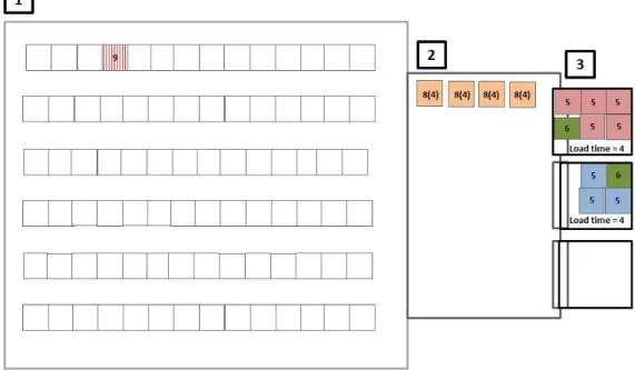
The process on which this research was built, can be explained with the help of figure 3.1. The figure shows the different steps that are taken when one (or more) item(s) is (are) ordered by the customer.

The process begins when a customer places an order. This order consists of at least one item. In figure 3.1a, three orders of different sizes have been placed. The colored items in the warehouse (location 1) represent the different items that have been ordered and, more in detail, the different orders that have been received are distinguished based on the different colors represented in the figure.

After an order has been placed, a due date (DD) is assigned to all the items of the specific order. This due date is expressed in the figure by the number inside the ordered item. The due date of an item is the latest time period an item should be shipped in order to arrive on time at its destination. Thus, an item should be loaded in a container and shipped before or at its due date in order to have an on-time delivery.

When the ordered items are available in the warehouse, an order picker can transport the items from the warehouse to the shelter space (location 2). As shown in figure 3.1b, all or-dered items have been moved to the shelter space. When the item is released to the shelter space, a release time (RT) is attached to the item corresponding to the time period the item arrives at the shelter space. In the figure, this is represented by the time period between brackets inside the ordered item.

Once the items have arrived at the shelter space, they can be selected to get loaded in a 7

(25)

Chapter 3. Problem description 8

container (figure 3.1c). The number of containers that can be loaded concurrently depends on the number of loading gates (location 3) that are present at the company’s warehousing infrastructure. These loading gates are areas where goods are loaded (or unloaded) into (out of) the containers.

The constructed mathematical model minimizes the total cost. This consists of a container loading cost, a backorder cost, and a lost sales cost. The container loading cost is a fixed cost that is included each time a container is shipped. When items are loaded in a container after their due date, a backorder cost is added. This penalty cost increases per time period the item is loaded too late. Even more drastically, when an ordered item is not loaded in a container during the total time horizon over which the model is evaluated, a lost sales cost is added for that item.

In figure 3.1b for example, an item, marked in red, has been ordered that is not available at the warehouse. Therefore, it might be possible that the item will not be available on time to get picked and loaded into a container before the due period of the item. In this case, a backorder cost will be added per time period the item is shipped too late. Another option is that the client will be informed that the product cannot be delivered. In this case, a lost sales cost will be added.

Several constraints must be taken into account in order to obtain a process model that can be used in practice. These constraints are expressed in the next chapter where the mathematical model is explained.

(26)

(a) Ordered items are located in the warehouse

(27)

(c) Picked items are loaded into a container

(28)

Chapter 4

Solution methodology

In this chapter, the details of the mathematical model will be elaborated. Although this mathematical model was constructed as a complete model, its discussion will be split up into three subsections. The first part concerns the basic feasibility constraints. It also includes decisions on the number of containers that will be loaded, and the selection of items that will be shipped. The second part deals with the exact positioning of the items in a container. Finally, the third part of this chapter concerns the order of loading the items in certain posi-tions of the container and the timing of loading them.

The notation of the used sets, parameters, and decision variables (DVs) in the model is de-scribed in table 4.1.

Sets

notation description

I the set of items

K the set of identical containers P the set of positions in a container

T the set of time periods

Parameters

li, wi, hi the length, width, and height of item i (cm)

vi the volume of item i (cm3)

qi the weight of item i (kg)

(29)

Chapter 4. Solution methodology 12

di the due time period of item i (period)

ri the release time period of item i (period)

(Lk, Wk, Hk) the length, width, and height of container k (cm)

Vk the volume capacity of container k (cm3)

Qk the weight capacity of container k (kg)

si the lost sales cost (e/item)

bi the backorder cost (e/period late)

ck the container loading cost (e/container used)

ti the time needed to load one item in a container (min)

E the number of employees

G the number of loading gates

rp the row number of position p

cp the column number of position p

lp the layer number of position p

DVs notation description ykst     

1, if container k with start time s and end time t is used 0, otherwise xikpt     

1, if item i is loaded at position p of container k at time period t 0, otherwise xi     

1, if item i is not loaded within the total time horizon considered 0, otherwise

˜

xi the number of time periods item i is shipped after its due time period (integer)

xs_pk the start of position p in x-direction in container k (integer) y_pks the start of position p in y-direction in container k (integer) z_pks the start of position p in z-direction in container k (integer) xe

pk the end of position p in x-direction in container k (integer)

y_pke the end of position p in y-direction in container k (integer) ze

(30)

Chapter 4. Solution methodology 13 notation description cpqk      1, if (y_pke - ys_qk)(y_qke - ys_pk)(z_pke - z_qks ) is positive 0, otherwise rpqk      1, if (xe_pk - xs_qk)(xe_qk - xs_pk)(z_pke - z_qks ) is positive 0, otherwise lpqk     

1, if (xe_pk - xs_qk)(xe_qk - xs_pk)(ye_pk - y_qks )(ye_qk - ys_pk) is positive 0, otherwise s1 pqk      1, if y_pke − ys qk is positive 0, otherwise s2_pqk      1, if y_qke − ys pk is positive 0, otherwise s3_pqk      1, if ze_pk− zs qk is positive 0, otherwise s4_pqk      1, if xe_pk− xs qk is positive 0, otherwise s5_pqk      1, if xe_qk− xs pk is positive 0, otherwise

Table 4.1: Overview of the sets, parameters, and decision variables

4.1 Feasibility constraints

M inimize ck X k∈K X s∈T X t∈T :t≥s ykst+ bi X i∈I ˜ xi+ si X i∈I xi (4.1)

The objective function of the model minimizes the total cost. A fixed cost, ck, is charged

(31)

shipped after their due period. This backorder cost increases linearly with the number of time periods the item is loaded too late. Furthermore, a lost sales cost per item, si, is added

for those items that are not loaded at the end of the examined time horizon. X k∈K X p∈P X t,ri∈T :t≥ri xikpt = 1 − xi ∀i ∈ I (4.2) X i∈I X p∈P xikpt ≤ M X s∈T :s≤t X t0_{∈T :t}0_≥t ykst0 ∀k ∈ K, ∀t, r_i ∈ T : t ≥ r_i (4.3) X s∈T X t∈T :t≥s tykst− di ≤ ˜xi+ M (1 − X p∈P X t,ri∈T :t≥ri xikpt) ∀k ∈ K, ∀i ∈ I (4.4) X s∈T X t∈T :t≥s ykst ≤ 1 ∀k ∈ K (4.5) X i∈I X t,ri∈T :t≥ri xikpt ≤ 1 ∀k ∈ K, ∀p ∈ P (4.6) X s∈T :s≤t X t0_{∈T :t}0_≥t X k∈K ykst0 ≤ G ∀t ∈ T (4.7) X i∈I X p∈P X t,ri∈T :t≥ri vixikpt ≤ Vk X s∈T X t∈T :t≥s ykst ∀k ∈ K (4.8) X i∈I X p∈P X t,ri∈T :t≥ri qixikpt ≤ Qk X s∈T X t∈T :t≥s ykst ∀k ∈ K (4.9) X s∈T X t∈T :t≥s ykst ≥ X s∈T X t∈T :t≥s y(k+1)st ∀k ∈ K (4.10) 1 − X t∈T :t≥s ykst ≥ X s0_{∈T :s}0_≤s X t∈T :t≥s0 y(k+1)s0_t ∀k ∈ K, ∀s ∈ T (4.11) ti X i∈I X p∈P X t∈T :t0_≥s,t0_≤t xikpt0 ≤ y_kst(t − s)E ∀k ∈ K, ∀s ∈ T , ∀t ∈ T : t ≥ s (4.12) ykst ∈ {0, 1} ∀k ∈ K, ∀s ∈ T , ∀t ∈ T : t ≥ s (4.13) xikpt ∈ {0, 1} ∀i ∈ I, ∀k ∈ K, ∀p ∈ P, ∀t, ri∈ T : t ≥ ri (4.14) xi ∈ {0, 1} ∀i ∈ I (4.15) ˜ xi ≥ 0 ∀i ∈ I (4.16)

Constraints 4.2 and 4.3 are linking constraints. The first constraint, constraint 4.2, makes it impossible for the decision variables xikpt and xi to both have the same value (0 or 1) for

a given item. If one of these decision variables equals 1, then the other one must equal 0 and vice versa. With the second linking constraint, constraint 4.3, a linkage is made between

(32)

the decision variables xikpt and ykst. An item can only be loaded into a specific container at

a certain time period if this container is open during that time period. Further, constraint 4.4 defines the integer variable ˜xi. When the item is shipped after its due time period, the

integer variable is assigned a value larger than zero. More specifically, it will be equivalent to the number of time periods the item has been shipped too late because of the minimization condition of the objective function. With constraint 4.5, it is stated that a container cannot be reopened. Constraint 4.6 defines that only one item can be loaded at every position in a container. The number of containers that can be loaded simultaneously depends on the number of gates available at the loading place. Therefore, constraint 4.7 restricts the number of containers to be opened at a time period to the number of gates. Further, constraints 4.8 and 4.9 limit the total volume and weight of all the items loaded into a container to the maximum volume capacity (VC) and weight capacity (WC) of the container. Constraint 4.10 is included for the ordering of the containers. The next container (k + 1) can only be used when container k has also been opened. Similarly, constraint 4.11 guarantees that the start time for loading container k + 1 cannot be smaller than the start time for loading container k. This is not a strict requirement, but breaks the symmetry of the model w.r.t. the selection of the container. Loading items in the container consumes time. The total time required to load the items depends on how long it takes (on average) to load an item in the container, and on the number of employees that load the container. The total time needed to load all the items in the container must be smaller than or equal to the planned time to load that container, as stated in constraint 4.12. Constraints 4.13 – 4.16 are domain constraints.

4.2 Positioning constraints

The positioning of items in a container will be explained with the help of a 2x2x2 represen-tation. Figure 4.1 displays the 2x2x2 model. The figure shows that eight positions can be filled in the container. Two columns, two rows, and two layers are identified in x-, y-, and z-direction respectively. A more detailed view on the structure is represented in figure 4.2.

The number of positions in each container is limited. The use of these defined positions in the containers is a rather theoretical construct, which allows to include the positioning of items as constraints in the mathematical model. However, the positions do not represent actual

(33)

positions of the items since their actual orientation in the container can vary. The position’s dimensions and orientation depend on the item that is placed at the specific position and on the other items that are loaded in the container.

Figure 4.1: 2x2x2 model representation

(34)

Chapter 4. Solution methodology 17 xe_pk≤ Lk ∀p ∈ P, ∀k ∈ K (4.17) ye_pk≤ Wk ∀p ∈ P, ∀k ∈ K (4.18) ze_pk≤ Hk ∀p ∈ P, ∀k ∈ K (4.19) xe_pk= xs_pk+X i∈I X t,ri∈T :t≥ri lixikpt ∀p ∈ P, ∀k ∈ K (4.20) ye_pk= y_pks +X i∈I X t,ri∈T :t≥ri wixikpt ∀p ∈ P, ∀k ∈ K (4.21) ze_pk= z_pks +X i∈I X t,ri∈T :t≥ri hixikpt ∀p ∈ P, ∀k ∈ K (4.22)

All the items must fit into the container. Therefore, the end of each zone in x-, y-, and z-direction must be smaller than or equal to the container size in the same direction. This is achieved using constraints 4.17 - 4.19. As previously stated, the position’s size depends on the specific item that is loaded in that position. The end of each zone in x-, y-, or z-direction corresponds to the start of that position in this dimension plus the length, width, or height of the item respectively. This is implemented using constraints 4.20 - 4.22.

xs_pk≥ xe_(p−1)k ∀p ∈ P : cp 6= 1, ∀k ∈ K (4.23) M s1_pqk≥ ye_pk− ys_qk ∀p, q ∈ P : (q > p ∧ lp 6= lq) ∨ (q > p ∧ lp= lq∧ rp6= rq), ∀k ∈ K (4.24) M s2_pqk≥ ye_qk− y_pks ∀p, q ∈ P : (q > p ∧ lp 6= lq) ∨ (q > p ∧ lp= lq∧ rp6= rq), ∀k ∈ K (4.25) M s3_pqk≥ z_pke − z_qks ∀p, q ∈ P : q > p, ∀k ∈ K (4.26) M s4_pqk≥ xe_pk− xs_qk ∀p, q ∈ P : q > p, ∀k ∈ K (4.27) M s5_pqk≥ xe_qk− xs_pk ∀p, q ∈ P : q > p, ∀k ∈ K (4.28)

(35)

Chapter 4. Solution methodology 18 cpqk ≥ s1pqk+ s2pqk+ s3pqk− 2 ∀p, q ∈ P : (q > p ∧ lp 6= lq) ∨ (q > p ∧ lp = lq∧ rp6= rq), ∀k ∈ K (4.29) rpqk ≥ s3pqk+ s4pqk+ s5pqk− 2 ∀p, q ∈ P : q > p ∧ rp 6= rq, ∀k ∈ K (4.30) lpqk ≥ s1pqk+ s2pqk+ s4pqk+ s5pqk− 3 ∀p, q ∈ P : q > p ∧ lp6= lq, ∀k ∈ K (4.31) xs_pk≥ xe_qk− (1 − cpqk)M ∀p, q ∈ P : (q > p ∧ c_p > cq∧ lp 6= lq)∨ (q > p ∧ cp > cq∧ lp = lq∧ rp 6= rq), ∀k ∈ K (4.32) xs_qk≥ xe pk− (1 − cpqk)M ∀p, q ∈ P : (q > p ∧ c_p ≤ c_q∧ l_p 6= l_q)∨ (q > p ∧ cp ≤ cq∧ lp = lq∧ rp 6= rq), ∀k ∈ K (4.33) ys_qk≥ ye pk− (1 − rpqk)M ∀p, q ∈ P : q > p ∧ r_p 6= r_q, ∀k ∈ K (4.34) z_qks ≥ z_pke − (1 − l_pqk)M ∀p, q ∈ P : q > p ∧ l_q6= l_q, ∀k ∈ K (4.35)

An important aspect that must be considered is that positions cannot overlap in the con-tainer. For positions that are not in the first column of the container, the start in x-direction will always be larger than or equal to the end of the previous position in this direction. This is represented by constraint 4.23. In the case of the 2x2x2 model, the start of position 2 cannot precede the end of position 1 in x-direction. The same reasoning holds for position 4 with respect to position 3, for position 6 with respect to position 5, and for position 8 with respect to position 7. This idea does not automatically hold for the y-, and z-direction, which will become clear later in this section.

Depending on the size of the items, it might become impossible in some cases to position the items relative to each other without either overlapping them or exceeding the container dimensions. To prevent this issue, the binary variables cpqk, rpqk, and lpqk have been

in-troduced. Binary variable cpqk will prevent overlap between items in x-direction. Similarly,

(36)

Because the different dimensions of the items must be taken into account to determine the potential overlap between items, the definition of these binary variables would result in the use of nonlinear constraints. This can also be observed in the notation table (table 4.1). To prevent this, five binary slack variables were introduced which make it possible to convert the nonlinear constraints into the desired linear shape. The definition of the slack variables is represented by constraints 4.24 - 4.28. Parameter M is a very large integer value. When the right-hand side of the constraint is positive, value 1 will be assigned to the slack variable. The definition of cpqk, rpqk, and lpqk follows in constraints 4.29 - 4.31. It is not required to

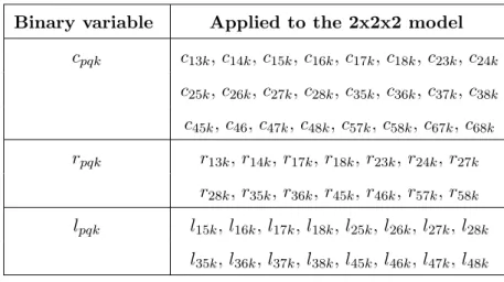
define these binary variables for each combination of the positions. For the 2x2x2 example, table 4.2 lists the generated combinations of cpqk, rpqk, and lpqk.

Binary variable Applied to the 2x2x2 model cpqk c13k, c14k, c15k, c16k, c17k, c18k, c23k, c24k c25k, c26k, c27k, c28k, c35k, c36k, c37k, c38k c45k, c46, c47k, c48k, c57k, c58k, c67k, c68k rpqk r13k, r14k, r17k, r18k, r23k, r24k, r27k r28k, r35k, r36k, r45k, r46k, r57k, r58k lpqk l15k, l16k, l17k, l18k, l25k, l26k, l27k, l28k l35k, l36k, l37k, l38k, l45k, l46k, l47k, l48k

Table 4.2: Overview of the binary variables cpqk, rpqk, and lpqk created for the 2x2x2 model

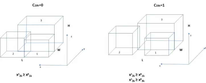
Constraints 4.32 and 4.33 define the start of a position in x-direction by making use of binary variable cpqk. In the case of a conflict between the two positions p and q in y-direction, the

items should be placed after each other in x-direction. Here, the loading order of the items must be respected. When the column number of position p is larger than the column number of position q, position p starts after position q in x-direction. Conversely, if the column number of position p is smaller than or equal to the column number of position q, position q starts after position p in x-direction. This can be clarified with the 2x2x2 example, which is further visualized in figure 4.3 . If binary variable c23k equals 1 and the column number of

(37)

at or after the end of position 3. When the binary variable is 0, the start of position 2 in x-direction only has to come after the end of position 1, as defined in constraint 4.23.

Figure 4.3: Example of the definition of binary variable cpqk

To determine the start of a position in y-direction, binary variable rpqk is used. When the

positions of different rows overlap in x-direction, rpqkis assigned a value of 1. In this case, the

start of position q must be larger than or equal to the end of position p in y-direction. This is obtained using constraint 4.34. This constraint is illustrated by figure 4.4 for positions 1 and 3 of the 2x2x2 model. When r13k is 1, the start of position 3 comes at or after the end

of position 1 in y-direction. Otherwise, if r13k is 0 (for example if c13k is 1, and thus the start

of position 3 comes after the end of position 1 in x-direction), the start of position 3 is not restricted by the end of position 1 in y-direction.

For defining the start of a position in z-direction, binary variable lpqk is needed. When two

positions of different layers overlap in x- and y-direction, meaning that they are stacked on top of each other, then the start of zone q must be larger than or equal to the end of zone p in z-direction. This is represented by constraint 4.35. In the case of the 2x2x2 example, position 1 and position 7 can be used to explain this constraint. Figure 4.5 shows that when

(38)

Figure 4.4: Example of the definition of binary variable rpqk

(39)

position 7 does not overlap with position 1 in both x- and y-direction, the start of position 7 is not influenced by the end of position 1 in z-direction. Nonetheless, it is influenced by the end height of position 3 since binary variable l37k equals 1. When there also is overlap with

position 1, then the start of position 7 must take into account the end of both position 1 and position 3 in z-direction.

4.3 Order of loading and timing constraints

The order in which the items are loaded into the container is important to take into account. Looking at the 2x2x2 model, it would be irrational to load an item at position 2 before loading an item at position 1 because this would result in not being able to use the container space of position 1. Thus, ordering constraints (constraints 4.36 - 4.40) have been added to the model.

X i∈I X t,ri∈T :t≥ri xikpt ≥ X i∈I X t,ri∈T :t≥ri xikqt ∀p, q ∈ P : (q > p ∧ lp= lq∧ rp = rq)∨ (q > p ∧ lp= lq∧ rp 6= rq∧ cp= cq), ∀k ∈ K (4.36) X i∈I X t,ri∈T :t≥ri xikqt+ (1 − cpqk)M ≥ X i∈I X t,ri∈T :t≥ri xikpt ∀p, q ∈ P : q > p ∧ lp = lq∧ rp6= rq∧ cp > cq, ∀k ∈ K (4.37) X i∈I X t,ri∈T :t≥ri xikpt+ (1 − cpqk)M ≥ X i∈I X t,ri∈T :t≥ri xikqt ∀p, q ∈ P : q > p ∧ lp = lq∧ rp6= rq∧ cp < cq, ∀k ∈ K (4.38) X i∈I X t,ri∈T :t≥ri xikpt ≥ X i∈I X t,ri∈T :t≥ri xikqt ∀p, q ∈ P : q > p ∧ lp 6= lq∧ rp= rq∧ cp = cq, ∀k ∈ K (4.39) X i∈I X t,ri∈T :t≥ri xikpt+ (1 − lpqk)M ≥ X i∈I X t,ri∈T :t≥ri xikqt ∀p, q ∈ P : q > p ∧ lp 6= lq∧ rp= rq∧ cp > cq, ∀k ∈ K (4.40)

(40)

At layer 1 of the 2x2x2 model, position 2 is always loaded after position 1 and position 4 after position 3. Also, position 3 is loaded only when an item is loaded at position 1. The same holds for position 4 with respect to position 2. This approach holds when the positions are in the same layer and in the same row, or when they are of different rows, but in the same column. This reasoning is represented by constraint 4.36. When the positions are of different rows and of different columns, the order in which the items are loaded depends on the binary variable cpqk. In constraint 4.37 and 4.38, it is defined what the order of loading

is, depending on how the positions of different rows and columns are situated relative to each other. For example, if binary variable c23k is 0, there is no rule of first loading an item in

position 2 or in position 3. If c23k is 1, then the start in x-direction of position 2 comes

after or at the end of position 3 according to constraint 4.32. In this case, an item should be loaded at position 3 first according to constraint 4.37. Constraint 4.39 and 4.40 are defined for positions having a different layer number. When the positions are not in the same layer and they are in the same row and in the same column, an item should be loaded first at the position of the lowest layer. In the 2x2x2 example, an item should be placed at position 1 before being able to load an item at position 5. For items of different layers positioned in the same row, the item in the lowest layer should be loaded first when binary variable lpqk is 1.

Not only the loading order must be considered. The load times of the items at these positions must also be taken into account. An item can only be loaded when it has been released to the shelter space. Additionally, we need to take the ordering of the positions into account. As previously stated, loading an item at position 2 at load time 4 would make it difficult to load an item at position 1 at load time 7. Constraint 4.41 has been added to facilitate the introduction of the load time per position to the model. The order of the load times at the positions of the container is represented in the model by constraints 4.42 - 4.45.

xs_qk≥ xs_pk

(41)

Chapter 4. Solution methodology 24 1 −X i∈I xikpt≥ X i∈I X t0_,r i∈T :t0≥ri,t0<t xikqt0 ∀k ∈ K, ∀p, q ∈ P : (q > p ∧ l_p = lq∧ rp = rq)∨ (q > p ∧ lp = lq∧ rp6= rq∧ cp = cq) ∨ (q > p ∧ lp6= lq∧ rp 6= rq∧ cp< cq)∨ (q > p ∧ lp 6= lq∧ rp= rq∧ cp < cq) ∨ (q > p ∧ lp6= lq∧ rp = rq∧ cp= cq), ∀t, ri∈ T : t ≥ ri (4.42) 1 −X i∈I xikqt+ (1 − cpqk)M ≥ X i∈I X t,ri∈T :t0≥ri,t0<t xikpt0 ∀k ∈ K, ∀p, q ∈ P : (q > p ∧ l_p = lq∧ rp 6= rq∧ cp > cq)∨ (q > p ∧ lp 6= lq∧ rp6= rq∧ cp > cq) ∨ (q > p ∧ lp6= lq∧ rp = rq∧ cp> cq), ∀t, r_i∈ T : t ≥ r_i (4.43) 1 −X i∈I xikpt+ (1 − cpqk)M ≥ X i∈I X t,ri∈T :t0≥ri,t0<t xikqt0 ∀k ∈ K, ∀p, q ∈ P : (q > p ∧ l_p= lq∧ rp6= rq∧ cp < cq)∨ (q > p ∧ lp6= lq∧ rp 6= rq∧ cp = cq), ∀t, ri ∈ T : t ≥ ri (4.44) 1 −X i∈I xikpt+ (1 − lpqk)M ≥ X i∈I X t0_,r i∈T :t0≥ri,t0<t xikqt0 ∀k ∈ K, ∀p, q ∈ P : (q > p ∧ lp6= lq∧ rp= rq∧ cp > cq)∨ (q > p ∧ lp6= lq∧ rp 6= rq∧ cp > cq) ∨ (q > p ∧ lp 6= lq∧ rp 6= rq∧ cp= cq), ∀t, ri∈ T : t ≥ ri (4.45)

Constraint 4.42 states that the position with position number (PN) p will be loaded before or at the same time as the position with PN q. This constraint holds for many cases, and will be explained with the 2x2x2 example. For positions of the same layer and the same row, such as position 1 and position 2 in the example, the load time of position 2 has to be larger than or equal to the load time of position 1. This also holds for positions of the same layer with different rows that are of the same column, such as position 1 and position 3. For positions of different layers that are in the same row and column, the load time of the position in the lowest layer must always be smaller than or equal to the load time of the position with the larger layer number. This is the case, for example, for position 1 and position 5 in the 2x2x2 example. Constraint 4.42 also holds for positions of different layers, with different rows and

(42)

the column number of the lowest layer position being smaller than the one of the higher layer position. This is the case for positions 1 and 8 in the 2x2x2 example. Finally, constraint 4.42 is also valid for positions of different layers with the same row number where the column number of the lowest layer position is smaller than the one of the higher layer position. For example, this holds for positions 1 and 6. In constraint 4.43 and 4.44, the binary variable cpqk will

determine the loading times of the positions relative to each other. For example in the 2x2x2 case, positions that are of the same layer, of different rows, and of different columns, such as position 2 and position 3, are considered with these constraints. When c23k is 0, the load

times of both positions can be the same, but an item can also be loaded at position 3 earlier or later than at position 2. When c23k is 1, the load time of position 2 should be larger than

or equal to the load time of position 3. Furthermore, for positions of different layers, binary variable lpqkwill be used in some cases to determine the loading times of the positions relative

to each other. This is defined by constraint 4.45. When lpqk is 1, the load time of the item in

the position of the lowest layer must be smaller than or equal to the load time of the item at the higher layer. This is for example the case for position 2 and position 5. If l25k equals 1,

then the load time of position 2 should be smaller than or equal to the load time of position 5.

To conclude this chapter, constraints 4.46 - 4.59 are the domain constraints of the variables linked to the positioning of the items in a container and their timing.

cpqk∈ {0, 1} ∀p, q ∈ P : (q > p ∧ l_p 6= l_q) ∨ (q > p ∧ lp= lq∧ rp 6= rq), ∀k ∈ K (4.46) rpqk∈ {0, 1} ∀p, q ∈ P : q > p ∧ r_p 6= r_q, ∀k ∈ K (4.47) lpqk∈ {0, 1} ∀p, q ∈ P : q > p ∧ l_p6= l_q, ∀k ∈ K (4.48) s1_pqk∈ {0, 1} ∀p, q ∈ P :(q > p ∧ l_p 6= l_q) ∨ (q > p ∧ lp = lq∧ rp 6= rq), ∀k ∈ K (4.49) s2_pqk∈ {0, 1} ∀p, q ∈ P : (q > p ∧ l_p 6= l_q) ∨ (q > p ∧ lp= lq∧ rp 6= rq), ∀k ∈ K (4.50)

(43)

Chapter 4. Solution methodology 26 s3_pqk ∈ {0, 1} ∀p, q ∈ P : q > p, ∀k ∈ K (4.51) s4_pqk ∈ {0, 1} ∀p, q ∈ P : q > p, ∀k ∈ K (4.52) s5_pqk ∈ {0, 1} ∀p, q ∈ P : q > p, ∀k ∈ K (4.53) xs_pk ≥ 0 ∀p ∈ P, ∀k ∈ K (4.54) y_pks ≥ 0 ∀p ∈ P, ∀k ∈ K (4.55) z_pks ≥ 0 ∀p ∈ P, ∀k ∈ K (4.56) xe_pk ≥ 0 ∀p ∈ P, ∀k ∈ K (4.57) y_pke ≥ 0 ∀p ∈ P, ∀k ∈ K (4.58) z_pke ≥ 0 ∀p ∈ P, ∀k ∈ K (4.59)

(44)

Chapter 5

Results and discussion

5.1 Datasets

Two datasets have been constructed to test the performance of the model. The datasets each consist of a set of 5 homogeneous containers, 24 positions per container, and 10 orders requesting for 20 items in total. The model was tested over 30 time periods with one time period being equal to 30 minutes. Thus, the model was tested over a total time horizon of 900 minutes.

The required data for the containers are the container number (CN), the dimensions of the container, the volume capacity (VC), and the weight capacity (WC). The used container dimensions are those from intermodal containers of a 20FT high cube container1. The weight capacity, however, is set much lower than the weight that a 20FT high cube container can bear in reality. This modification is applied to ensure that the weight capacity constraint (constraint 4.9) is considered.

A set of 20 heterogeneous items has been created for each dataset. The required data per item consists of the item number (IN), the item’s dimensions, the item’s weight, and the order number (ON) to which it belongs. The length, width, and height of the items were randomly chosen in the interval of 75–150 cm. The volume of each item is equivalent to the multiplication of its three dimensions. The weight is calculated by multiplying the volume of the item by 0,3 g/cm3.

1_{https://www.mainfreight.com/global/en/basics/freight-basics-shipping-container-specifications.aspx}

(45)

Chapter 5. Results and discussion 28

The due date of an item is determined by its corresponding order. Between one to five items can be requested per order. The order time (OT) was randomly generated on the complete time horizon. The due date (DD), representing the latest time period the items of an order need to be shipped in order to arrive on time at the customer, corresponds to the order time plus 10 time periods (i.e. 300 minutes). The release time (RT) of the items is equivalent to the order time plus 120 minutes.

As previously explained, the position data depends on the specific dimensions of the items in the dataset. For the position data, the position number (PN) is required. The number of positions in a container, further subdivided in the number of rows, columns, and layers is a rather theoretical construct aimed at facilitating the implementation of positioning the items as constraints in the mathematical model. The number of positions in the container has been determined based on the cumulative sum of the smallest item lengths, widths, and heights in both datasets. The largest number of rows, columns, and layers needed per container equals the sum of the smallest items that fit into the respective container dimension without exceeding it.

The complete content of the data can be found in appendix A for dataset 1 and in appendix B for dataset 2. A short summary of the content is represented in table 5.1.

Container data

# Containers Length (cm) Width (cm) Height (cm) VC (cm3₎ _{WC (kg)}

5 589 235 269 37,233,635 5000

Item data

# Items Length (cm) Width (cm) Height (cm) Volume (cm3) WC (kg)

20 [115-150] [75-120] [85-120] li* wi* hi 0.0003 kg / cm3

Order data

# Orders OT (min) DD (min) RT (min) Items ordered (items)

10 [0-900] Order time + 300 Order time + 120 [0-5]

Position data per container

# Positions # Columns # Rows # Layers

24 4 3 and 2 2 and 3 Time horizon Total time (min) Total time (periods) Possible start periods (periods) Possible end periods (periods) Possible load

time periods (periods)

900 30 30 30 30

(46)

5.2 Results

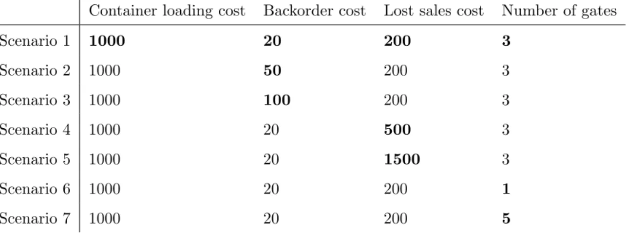
The aim of this report was to construct an ILP container loading model taking the release times and due dates of the ordered items into account. In order to evaluate the impact of certain parameters in the model, the model was tested for seven different scenarios where one parameter changed in value per scenario. Table 5.2 provides an overview of the different scenarios that have been tested. Scenario 1 is the base scenario to which all other scenarios will be compared. All scenarios have been solved using Gurobi 8.1.1 and the computation time was limited to three hours per scenario.

For the parameter testing of this mathematical model, the time needed to load an item into the container (ti) and the number of employees (E) were not taken into account. These

parameters were previously mentioned in constraint 4.12. Parameter testing would be useful for tiand E when all timing was set in the same unit of measurement. However, this model is

evaluated based on time periods of 30 minutes with the result that this constraint will become redundant when it only takes 1-3 minutes to load an item in a container.

Container loading cost Backorder cost Lost sales cost Number of gates

Scenario 1 1000 20 200 3 Scenario 2 1000 50 200 3 Scenario 3 1000 100 200 3 Scenario 4 1000 20 500 3 Scenario 5 1000 20 1500 3 Scenario 6 1000 20 200 1 Scenario 7 1000 20 200 5

Table 5.2: Overview of the different scenarios tested

First, it should be stressed that the results presented in this section should be interpreted with great caution. After a computation time of three hours, no optimal solution was found for any of these scenarios. Furthermore, the solution gap was not constant for the different scenarios. This gap represents the relative difference between the objective bound and the incumbent solution objective. An optimal solution is only found if the gap is equivalent to

(47)

0%. The solution gap of each scenario per dataset is represented in table 5.3.

Dataset 1 Dataset 2 Scenario 1 28.6 % 25.9 % Scenario 2 33.3 % 33.3 % Scenario 3 39.4 % 33.3 % Scenario 4 33.3 % 33.3 % Scenario 5 33.3 % 46.5 % Scenario 6 41.2 % 27.0 % Scenario 7 23.7 % 33.3 %

Table 5.3: Solution gap per scenario for dataset 1 and dataset 2

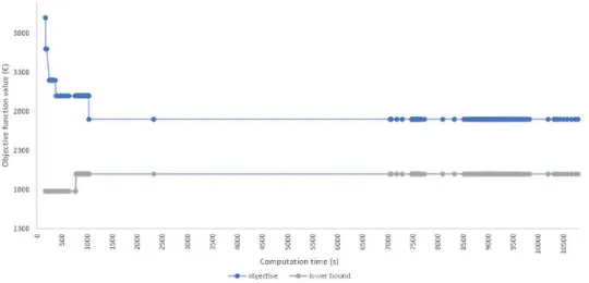
An increased computation time, however, does not lead to an optimal result. For most results, the gap remained constant after one hour of computing. This behavior can be observed in figures 5.1 and figure 5.2, which show the progression of scenario 1 for dataset 1 and dataset 2. For both datasets, the gap remained constant after one hour of computing for the first scenario. Nonetheless, some scenarios did show a shift in the solution gap after one hour of computing. This is why each scenario was executed for three hours instead of one hour.

(48)

Figure 5.2: Time lapse of computation scenario 1 dataset 2

The obtained values of the variables per scenario are represented in appendix C for dataset 1 and in appendix D for dataset 2. These are further discussed in the following paragraphs.

Objective function value

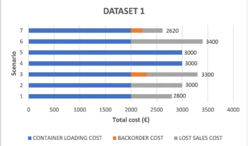
The objective function of the mathematical model minimizes the sum of the container load-ing cost, the backorder cost, and the lost sales cost. In appendix E, tables are included that compare the data of the different scenarios for each dataset. Tables 25 and 26 represent the objective function values per scenario per dataset. These tables are visualized by figures 5.3 and 5.4. For dataset 1, the lowest objective function value was obtained in scenario 7, while the lowest value for dataset 2 was obtained in scenario 1.

In scenario 2 and 3, the backorder cost (bi) was increased. For both datasets, this resulted in

an increase in the objective function value and an increase in the lost sales cost. For scenarios 4 and 5, the lost sales cost (si) was increased with the intention to obtain as few non-shipped

items as possible. For both datasets, all items were loaded into a container for both scenarios 4 and 5. This resulted in opening an extra container and therefore an increased container loading cost was observed. For scenario 6, the number of gates was reduced from three gates to one gate. For dataset 1, this resulted in an increase in lost sales resulting in a remarkably larger objective function value. For dataset 2, this led to an increase in backorder costs, and the increase in objective function value was less substantial. For scenario 7, the number

(49)

of gates was increased from three to five gates. For dataset 1, this resulted in the lowest objective function value of all scenarios, with a decrease in lost sales cost and an increase in backorder cost compared to scenario 1. For dataset 2, the objective function value increased with an increase in the lost sales cost compared to scenario 1.

For each scenario of both datasets, with the exception of scenario 7 for dataset 1, the solution gap was larger than the gap of the base scenario (scenario 1) indicating a larger complexity for solving the model.

Figure 5.3: Objective function value per scenario for dataset 1

(50)

Timing

In the literature review chapter, it was discussed that relative priorities give the possibility of a better use of the available container space. However, not each item can always be shipped earlier than needed. The focus of the model was on taking the release time and due date of each ordered item into account. Thus, an item can only be sent when the item has already been released to the shelter space.

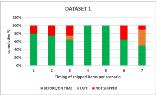
Tables 27 and 28 in appendix E show the percentage of units that were loaded before, at, or after their due date for dataset 1 and dataset 2. Also, the percentage of the items that were not loaded at all are represented in these tables. These tables are further visualized in figures 5.5 and 5.6 for dataset 1 and dataset 2 respectively. In these figures, early and on-time deliveries were combined since both lead to an on-time delivery to the customer.

Increasing the backorder cost (scenarios 2 and 3) led to an increase in items which are not shipped for both datasets. When the backorder cost is increased, it seems to be more beneficial to not send the items rather than to send them late. Of course, this must be interpreted with caution because the solution gaps are larger for scenario 2 and 3 than the one of the base scenario for both datasets. Increasing the lost sales cost (scenarios 4 and 5) resulted in all items to be shipped. For dataset 1, this leads to an increase in early deliveries compared to the base scenario. For dataset 2, the small increase in lost sales cost (scenario 4) led to an increase in early and on-time deliveries, with the result that all items were shipped on time. For the larger lost sales cost (scenario 5), more items were shipped late in order to make sure that all items were shipped. Decreasing the number of gates to a single gate (scenario 6) led to different results for both datasets. For dataset 1, it resulted in an increase in non-shipped items while all items were shipped for dataset 2, but more items were shipped late compared to the base scenario. When the number of available gates was increased to five gates (scenario 7), again, different results were obtained for both datasets. Dataset 1 had less non-shipped items compared to the base scenario, with more items being shipped late. For dataset 2, there is an increase in non-shipped items, but all items that were shipped had an on-time delivery to the customer.

(51)

Figure 5.5: Timing of items shipped for dataset 1

(52)

Positioning

The positioning of the items in the container was included as linear constraints in the model. For scenario 1 of both dataset 1 and dataset 2, figures 5.7 and 5.8 show the loaded items in container 1 and container 2 respectively. These figures were constructed based on the information of tables 9 and 17 of appendix C and D.

At first sight, it can be noted that none of these containers are completely filled. Quite some empty spaces can be observed. As explained before, this is related to the release times and due dates of the items. In the model, a trade-off is made between the container loading cost, the backorder cost, and the lost sales cost. As a result, if the release time and the due dates of the ordered items are close to each other, the chances are higher to have more items to be loaded into the same container. When the difference in timing becomes larger, the backorder cost might become too large and the decision could be made to open another container or to let items be not-shipped.

Another aspect that can be noted, is that some items are floating in the container. This can be explained by how the constraints were formulated in the model. In constraints 4.35 and 4.56, it was only imposed that the start in z-direction had to be larger than or equal to the end of the underlying item, meaning that there is a possibility to have a floating item in the container. In practice, however, it is possible to store the items on top of each other without having to change to coordinates in x- and y-direction.

Complexity

At the beginning of this chapter, it was stressed that no optimal solution was found for any of the computed scenarios. In this section, it is investigated what makes this model so complex such that no optimal solution can be found after three hours of computing. More specifically, it is investigated what the impact is on the complexity of the model of the number of positions in a container and of the spread of timing between orders.

For this purpose, three extra datasets have been constructed. One dataset (dataset 3) limits both the number of positions in a container and the spread of timing between the orders. The next dataset (dataset 4) has a larger number of positions while the spread of timing remains

(53)

Figure 5.7: Positioning of items of scenario 1 for dataset 1

(54)

small. Further, the last dataset (dataset 5) consist of little positions in a container while the spread of timing between orders is larger. The details of these datasets can be found in tables 29 - 35 of appendix F. All the different scenarios (table 5.2) have been tested for these datasets and the computation time was each time set to three hours.

Dataset 1 Dataset 2 Dataset 3 Dataset 4 Dataset 5

Scenario 1 28.6 % 25.9 % 0.0 % 8.0 % 3.9 % Scenario 2 33.3 % 33.3 % 0.0 % 13.6 % 16.7 % Scenario 3 39.4 % 33.3 % 0.0 % 0.0 % 1.3 % Scenario 4 33.3 % 33.3 % 0.0 % 0.0 % 1.3 % Scenario 5 33.3 % 46.5 % 0.0 % 0.0 % 1.3 % Scenario 6 41.2 % 27.0 % 0.0 % 0.0 % 2.0 % Scenario 7 23.7 % 33.3 % 0.0 % 0.0 % 1.2 %

Table 5.4: Overview of the solution gap per scenario for each dataset

In table 5.4, the solution gaps per scenario for each dataset are represented. It can be noticed immediately that the solution gaps of dataset 1 and dataset 2 are remarkably larger than the ones of the other three datasets. Thus, the datasets with both a larger number of positions per container and a wider spread in the timing of orders are harder to solve for the model. For dataset 3, with little positions and little spread in timing, optimal solutions have been found for all the scenarios. Furthermore, these optimal solutions were obtained in less than 30 minutes of computation time per scenario. For dataset 4, with many positions and little spread in timing, optimal solutions have been found in five cases, and smaller solution gaps are obtained for the other two scenarios compared to dataset 1 and dataset 2. Additionally, a computation time of approximately one hour was needed for each scenario to construct the obtained results. For dataset 5, consisting of a small number of positions per container and a large spread in timing between orders, no optimal solutions were found. Nonetheless, the solution gaps are smaller compared to those of dataset 1 and dataset 2.

Thus, it can be concluded that the timing of the orders has a remarkable impact on the complexity of solving the model meaning that the model will perform better in case orders are made frequently. Additionally, the number of positions in a container adds to the complexity

(55)

of the model. As a result, the model is hardest to solve when there are many positions per container and there is a large spread in timing of orders occurring.

5.3 Discussion

Six possible orientations exist according to which a rectangular item can be positioned in a container. For this study, only a single orientation was permitted for each item in both the horizontal and vertical direction. Thus, the items cannot be rotated to be loaded in the container. Depending on the type of items to be loaded, orientation constraints could result in a more efficient use of the available volume of the container. For fragile items, often only a single vertical orientation is permitted with no restriction on the horizontal direction. This allows for 90◦ rotations of the items on the horizontal plane as described in the heuristic procedure of Haessler & Talbot (1990) and in the overview of Iori & Martello (2010). For non-fragile items, it could be beneficial to have no restrictions on the orientation of the items in the container. When all items can be freely rotated, the largest solution freedom exists (Parre˜no et al. (2008)). Recently, the paper of Kurpel et al. (2020) proposed a mathematical formulation that considers the six possible orientations of an item. This is described for both input minimization problems as for output maximization problems.

In this study, weight distribution constraints have not been included in the model. Weight distribution constraints require that the weight of the cargo is spread as evenly as possible across the container floor. By balancing the load, the risk is reduced that the cargo shifts while the container is moved. To achieve an even weight distribution, the center of gravity of the load should be as close as possible to the geometrical mid-point of the container floor or should not exceed a certain distance as studied by Gehring & Bortfeldt (1997), Bortfeldt & Gehring (2001), and Liu et al. (2011).

The stability of the items is not explicitly considered in this study. Stability of the cargo should be guaranteed in order to prevent damage of the loaded items during transportation. Vertical stability (also called static stability) prevents items from falling down onto the con-tainer floor. This deals with the situation when the concon-tainer is not being moved and describes the capacity of the load to withstand the gravitational force as discussed by Junqueira et al.

(56)

(2012). Horizontal stability (also called dynamic stability) assures that items cannot shift while the container is being moved as explained in Bischoff & Ratcliff (1995). It refers to the capacity of the items to withstand the inertia of their bodies (Junqueira et al. (2012)).

Project scheduling is concerned with single-item or small batch production where there is a scarcity of resources available when scheduling dependent activities over time. As explained by Brucker et al. (1999), project scheduling problems in general are really challenging from a computational point of view. Project networks might have varying processing times depending on a time-cost trade-off. A link between project scheduling and container loading is possible with this model because it takes the release time of the items into account. Items can only be loaded when they are released to the shelter space. When items are ordered, but are not in storage, they cannot be released to the shelter space.

(57)

Chapter 6

Conclusions

The aim of this thesis was to make an integer linear programming (ILP) container loading model taking the timing aspect into account that is related to the loaded items. In this multi-container loading problem, both the time period when items are released to the shelter space and the due time period of the items were considered in the construction of the mathe-matical model. Furthermore, the positioning of the items in the containers was implemented by means of linear constraints.

Representing a multi-container loading problem completely as an ILP model does not occur frequently in the existing literature. Similarly, heuristic procedures are often used for the posi-tioning of the cargo inside the containers in favor of a mathematical formulation in the model.

To test the performance of the model, two datasets have been constructed for which each time seven scenarios were executed. In each scenario, one parameter value was changed to see its impact on the results of the model. From this, it was observed that the model was too complex to find an optimal solution in a time limit of three hours of computation time. Moreover, the solution gap varied depending on the changing parameter values in the different scenarios. Further, three additional datasets were created to trace the origin of the complexity in the model. From the results, it was concluded that the main cause of the complexity lies in the spread of timing between orders. Also, an increase in the number of positions per container adds to the difficulty of getting an optimal solution within a computation time of three hours.

(58)

References

M. Alonso, R. Alvarez-Valdes, M. Iori & F. Parre˜no (2019). Mathematical models for multi container loading problems with practical constraints. Computers & Industrial Engineering, 127:722–733.

M. Alonso, R. Alvarez-Valdes, M. Iori, F. Parre˜no & J. Tamarit (2017). Mathematical models for multicontainer loading problems. Omega, 66:106–117.

J. A. Bennell, L. S. Lee & C. N. Potts (2013). A genetic algorithm for two-dimensional bin packing with due dates. International Journal of Production Economics, 145(2):547–560. E. E. Bischoff & M. Ratcliff (1995). Issues in the development of approaches to container

loading. Omega, 23(4):377–390.

A. Bortfeldt & H. Gehring (2001). A hybrid genetic algorithm for the container loading problem. European Journal of Operational Research, 131(1):143–161.

A. Bortfeldt & G. W¨ascher (2013). Constraints in container loading–a state-of-the-art review. European Journal of Operational Research, 229(1):1–20.

P. Brucker, A. Drexl, R. M¨ohring, K. Neumann & E. Pesch (1999). Resource-constrained project scheduling: Notation, classification, models, and methods. European journal of operational research, 112(1):3–41.

C. Chen, S.-M. Lee & Q. Shen (1995). An analytical model for the container loading problem. European Journal of Operational Research, 80(1):68–76.

A. P. Davies & E. E. Bischoff (1999). Weight distribution considerations in container loading. European Journal of Operational Research, 114(3):509–527.

(59)

References 42

H. Gehring & A. Bortfeldt (1997). A genetic algorithm for solving the container loading problem. International transactions in operational research, 4(5-6):401–418.

R. W. Haessler & F. B. Talbot (1990). Load planning for shipments of low density products. European Journal of Operational Research, 44(2):289–299.

Y.-H. Huang, F. Hwang & H.-C. Lu (2016). An effective placement method for the single container loading problem. Computers & Industrial Engineering, 97:212–221.

M. Iori & S. Martello (2010). Routing problems with loading constraints. Top, 18(1):4–27. L. Junqueira, R. Morabito & D. S. Yamashita (2012). Three-dimensional container

load-ing models with cargo stability and load bearload-ing constraints. Computers & Operations Research, 39(1):74–85.

F. Koblasa & M. Vavrousek (2018). Bin packing and scheduling with due dates.

D. V. Kurpel, C. T. Scarpin, J. E. P. Junior, C. M. Schenekemberg & L. C. Coelho (2020). The exact solutions of several types of container loading problems. European Journal of Operational Research, 284(1):87–107.

J. Liu, Y. Yue, Z. Dong, C. Maple & M. Keech (2011). A novel hybrid tabu search approach to container loading. Computers & Operations Research, 38(4):797–807.

N.-C. Liu & L. Chen (1981). A new algorithm for container loading. In Compsac 81-5th International Computer Software and Applications Conference Proceedings, pp. 292–299. IEEE Press Chicago,(IL).

S. Martello, D. Pisinger & D. Vigo (2000). The three-dimensional bin packing problem. Oper. Res., 48:256–267.

D. A. Mart´ınez, R. Alvarez-Valdes & F. Parre˜no (2015). A grasp algorithm for the container loading problem with multi-drop constraints. Pesquisa Operacional, 35(1):1–24.

R. K. Mavi, M. Goh, N. K. Mavi, J. Ferry, K. Brown, S. Biermann & A. A. Khanfar (2020). Cross-docking: A systematic literature review. Sustainability, 12(11):4789.