applications
Academic year 2019-2020
Master of Science in Information Engineering Technology
Master's dissertation submitted in order to obtain the academic degree of
Counsellors: Dwight Kerkhove, Tom Goethals
Supervisors: Prof. dr. Bruno Volckaert, Prof. dr. ir. Filip De Turck
Student number: 01502396During this semester I have been working on this dissertation that ends my Master of Science in Information Engineering Technology at the Ghent University. This would not have been possible without the help of the following people.
First of all I would like to thank my counsellors Dwight Kerkhove and Tom Goethals for guiding me, answering all my questions and giving me helpful tips and tricks.
I want to thank Prof. dr. Bruno Volckaert and Prof. dr. ir. Filip De Turck for allowing me to choose this interesting subject for my dissertation.
Finally I want to thank my parents, Peter Surmont and Ann Verschelde, for giving me the opportunity to obtain this degree and my girlfriend, Justine Opsomer, for the support.
Cédric Surmont
De auteur geeft de toelating deze masterproef voor consultatie beschikbaar te stellen en delen van de masterproef te kopiëren voor persoonlijk gebruik. Elk ander gebruik valt onder de bepalingen van het auteursrecht, in het bijzonder met betrekking tot de verplichting de bron uitdrukkelijk te vermelden bij het aanhalen van resultaten uit deze masterproef.
The author gives permission to make this master dissertation available for consultation and to copy parts of this master dissertation for personal use. In all cases of other use, the copyright terms have to be respected, in particular with regard to the obligation to state explicitly the source when quoting results from this master dissertation.
Analyse van video streaming in industriële IoT applicaties (NL)
door Cédric Surmont Academiejaar 2019-2020
Universiteit Gent
Faculteit Ingenieurswetenschappen en Architectuur
Promotoren: Prof. dr. Bruno Volckaert, Prof. dr. ir. Filip De Turck Begeleiders: Dwight Kerkhove, Tom Goethals
Abstract - NL
Het Internet of Things groeit zeer snel en steeds meer apparaten zijn verbonden met het Internet. Ook in de industrie wordt dit concept gebruikt, bijvoorbeeld in het City of Things1 project van
imec. In dat project worden zeer veel sensoren geïnstalleerd in Antwerpen en met die data kunnen allerlei experimenten en voorspellingen gedaan worden. Het grootste deel van deze sensoren produceren numerieke data die gemakkelijk verwerkt en opgeslagen worden. Een andere soort data, die ook moet verwerkt worden, bestaat uit video beelden, die geproduceerd worden door de vele security camera’s in de stad.
De beelden van deze camera’s, en ook andere zoals inspectiecamera’s in de industrie, ondergaan meestal een transcoding proces vooraleer de data kan gebruikt worden. Dit (live) proces verwerkt de inkomende videobeelden van verschillende bronnen en zet dit om naar de gewenste output. Deze output kan dan live getoond worden, soms in verschillende kwaliteiten, of wordt opgeslagen om later opgevraagd te worden. Dergelijke processen vormen een zware last op de architectuur en de verschillende aspecten ervan zullen in deze scriptie geanalyseerd worden.
Trefwoorden: Video streamen, transcoden, live, compressie, automatisatie, bash, codec
Analysis of video streaming in industrial IoT applications (EN)
by Cédric Surmont Academic Year 2019-2020
University Ghent
Faculty of Engineering and Architecture
Supervisors: Prof. dr. Bruno Volckaert, Prof. dr. ir. Filip De Turck Counsellors: Dwight Kerkhove, Tom Goethals
Abstract - EN
The Internet of Things is a rapidly growing space. More and more devices get smarter and are connected to the Internet. In an industrial context IoT is widely used to obtain huge amounts of sensor data from machines, which is analyzed and distilled into useful metrics such as maintenance prediction, anomaly detection and performance. Imec’s City of Things project2
is the perfect example of an industrial IoT environment.
One example of these machines in the City of Things project that transfer data for processing are the CCTV cameras. These cameras produce video files 24/7 that have to be available for live monitoring and Video On Demand (VOD) services. Processing video streams require a different kind of architecture than other sensor data. Therefore, in this dissertation, the effects of video streaming in an industrial IoT context will be analyzed. Specifically, the live transcoding process that takes place at the main framework will be tested and experimented on. This process accepts its input video from multiple sources and transforms each input to an output format with certain well defined properties. The different aspects of this operation will be thoroughly inspected and tested for multiple scenarios.
Keywords: Video streaming, transcoding, live, compression, automation, bash, codec
Analyse van video streaming in industriële IoT
applicaties
Cédric Surmont
Promotoren: Bruno Volckaert, Filip De Turck Begeleiders: Dwight Kerkhove, Tom Goethals
Abstract— Dit artikel analyseert het live transcoding proces dat gebruikt wordt om live video aan te bieden. Dit proces zal worden opgezet om de videobeelden van het City of Things project van imec te verwerken. De huidige opstelling zorgt voor een te grote last op de CPU’s van de architectuur en dit zorgt ervoor dat buffers vollopen waardoor het proces stil kan vallen. De invloed van verschillende pa-rameters, opties en codecs op de performantie zal onderzocht worden. Kernwoorden— Video streamen, transcoden, live, compressie, au-tomatisatie, bash, codec
I. Introductie
H
ET Internet of Things groeit zeer snel en steeds meerapparaten zijn verbonden met het Internet. Ook in de industrie wordt dit concept gebruikt, bijvoorbeeld in het City of Things project van imec. In dat project wor-den zeer veel sensoren geïnstalleerd in Antwerpen en met die data kunnen allerlei experimenten en voorspellingen ge-daan worden. Het grootste deel van deze sensoren produ-ceren numerieke data die gemakkelijk verwerkt en opgesla-gen worden. Een andere soort data, die ook moet verwerkt worden, bestaat uit video beelden, die geproduceerd wor-den door de vele security camera’s in de stad.De beelden van deze camera’s, en ook andere zoals inspec-tiecamera’s in de industrie, ondergaan meestal een trans-coding proces vooraleer de data kan gebruikt worden. Dit (live) proces verwerkt de inkomende videobeelden van ver-schillende bronnen en zet dit om naar de gewenste output. Deze output kan dan live getoond worden, soms in verschil-lende kwaliteiten, of wordt opgeslagen om later opgevraagd te worden. Dergelijke processen vormen een zware last op de architectuur en zullen in dit artikel geanalyseerd wor-den.
II. Probleemstelling
Het transcoding proces bestaat uit twee fases: De bin-nenkomende beelden worden eerst gedecodeerd naar een raw video formaat zoals YUV. Vanuit dit formaat kan de video terug geëncodeerd worden tot de gewenste output. De technologieën die dit enCOderen en DECoderen uitvoe-ren worden codecs genoemd. Deze codecs zijn implementa-ties van gestandaardiseerde formaten, de meest gebruikte is de H.264 standaardisatie. Dergelijke formaten leggen de methodes vast waarmee de video’s gecomprimeerd kunnen worden. Veel gebruikte methodes zijn wiskundige transfor-maties zoals de Discrete Cosine Transform (DCT), gebruikt in de H.264 en H.265 specificaties. Deze transformatie kan
een reeks data uitdrukken in een som van cosinus functies met verschillende frequenties. Deze som heeft specifieke ei-genschappen die veel gemakkelijker gecomprimeerd kunnen worden met bijvoorbeeld Huffman coding. De implemen-taties van de H.264 specificatie en haar opvolger H.265 die in deze scriptie gebruikt worden zijn respectievelijk libx264 en libx265.
Dit geheel kan zeer snel worden uitgevoerd door een computer, maar veel verschillende aspecten beïnvloeden dit proces. De verschillende eigenschappen van de input zoals de resolutie van de beelden, de frame rate, maar ook de in-houd spelen een rol in de snelheid waarmee een CPU deze transcoding kan uitvoeren.
III. Testomgeving
Met de hulp van tools zoals Docker, FFmpeg en de Virtual wall van imec kan dit proces grondig onderzocht worden door middel van verschillende experimenten. Het transcoding proces wordt telkens uitgevoerd in een custom Docker container. Deze container heeft als basis de Ubuntu 18.04 image en is uitgebreid met de FFmpeg en youtube-dl packages. Door middel van een entrypoint script, ge-schreven in bash, wordt bij de start van deze container een meegegeven video file doorgepipet, zoals een livestream, naar het live transcoding script. Dit transcoding script be-staat voornamelijk uit een groot FFmpeg commando dat een DASH1 output genereert. DASH splits een video
be-stand in korte fragmenten die afzonderlijk over het internet kunnen verstuurd worden om video streaming mogelijk te maken zonder eerst de volledige video te moeten downloa-den. Dit FFmpeg commando voert de transcoding uit met de verschillende meegegeven parameters en opties. Om het effect van deze opties te testen wordt in elk experiment telkens één optie gewijzigd en worden de resultaten verge-leken met de originele. Niet enkel de opties van het proces worden onderzocht maar ook de invloed die verschillende soorten input hebben.
Deze resultaten bestaan uit onder andere de peak signal-to-noise ratio (PSNR) en de structural similarity index (SSIM) om de kwaliteit van de output te kunnen meten. Deze waardes worden per frame berekend en geven een idee van de visuele kwaliteit van de geproduceerde bestanden zonder ze effectief aan mensen te moeten tonen. Een an-dere metriek die gemeten wordt is het CPU-gebruik dat het proces inneemt. Dit is belangrijk om te kunnen
Deze resultaten worden ook gemeten en berekend door middel van bash scripts. De status informatie van de FFmpeg processen kan uit het /proc filesystem van Ubuntu gehaald worden en de kwaliteitsmetrieken kunnen met een ander geautomatiseerd FFmpeg proces berekend worden.
Ieder experiment onderzoekt één specifiek aspect van het proces en bestaat uit verschillende testen, die elk een be-paalde waarde van dat aspect invullen. Om meer gemid-delde resultaten te behalen wordt elke test 5 keer uitge-voerd onder identieke omstandigheden, zo wordt de invloed van uitschieters beperkt.
IV. Resultaten A. Eerste experiment
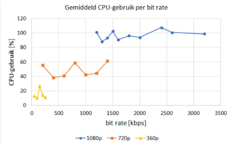
De eerste soort beelden die getest worden zijn gemaakt door een verkeerscamera boven de oprit van een snelweg. Dit zorgt voor video materiaal met zeer veel beweging door-dat er op elk moment verschillende voertuigen in beeld zijn. Na een eerste experiment, dat de invloed van verschil-lende output bit rates onderzocht per resolutie, is het dui-delijk dat de bit rate niet echt een lineair verband heeft met het CPU-gebruik. Zoals te zien is op Figuur 1 is er wel een hoger CPU-gebruik naarmate de resolutie van de video stijgt.
Fig. 1. CPU-gebruik per output bit rate.
Resultaten voor 3 resoluties: 1080p, 720p en 360p
Dit experiment resulteerde in uitvoeringstijden van ge-middeld 126 seconden voor video’s van slechts 120 secon-den. Dit wijst er op dat de snelheid van het transcoden te laag ligt om dit voor een lange tijd vol te houden zonder de buffer te laten vollopen. Dit wordt opgelost door de ’-re’ optie, die ervoor zorgt dat de input in real-time wordt verwerkt, weg te laten in het transcoding script, wat ook voordelig blijkt te zijn voor de performantie. Deze optie wordt al gebruikt in het script dat de video’s doorgeeft aan het transcoding script, dus de real-time simulatie wordt daar al verzorgd.
De libx264 codec heeft nog zeer veel andere opties en encoding settings die het proces kunnen aanpassen. Om de gebruikers het gemakkelijker te maken bestaan er preset opties die deze settings bundelen. Een snellere preset zorgt ervoor dat de encoding sneller kan gebeuren, maar zorgt voor een mindere graad van compressie.
Deze presets werden getest in verschillende experimenten en hadden ook een significante invloed op zowel de kwaliteit als het CPU-gebruik. Tragere presets zorgden niet voor een tragere uitvoering maar wel voor meer CPU-gebruik dan de snellere presets. Elke output had dezelfde bit rate, maar tragere presets creëerden minder grote bestanden, wat wijst op een betere compressiegraad, waarvoor dus ook meer re-kenkracht nodig is. Deze bestanden hadden ook betere PSNR en SSIM index waarden dan de snellere presets wat wijst op een betere kwaliteit.
De vorige experimenten hadden telkens een vast output bit rate ingesteld, maar er is ook een andere mogelijkheid om de output te specificeren: CRF waarden. Deze Con-stant Rate Factor is een geheel getal tussen 0 en 51 dat de algemene kwaliteit van een video voorstelt. Hoe lager deze waarde, hoe beter de kwaliteit van de video zal zijn. De libx264 en libx265 codecs voorzien ook een optie om deze waarde in te stellen voor de output. In deze experimenten worden de waarden 23 (de standaard waarde), 25, 27 en 30 getest.
Zoals verwacht zijn de PSNR en SSIM index hoger voor lagere CRF waarden. Om deze hogere kwaliteit te kunnen produceren is er ook meer CPU kracht nodig. Doordat deze CRF optie een bepaalde kwaliteit garandeert kan ze gebruikt worden als er voldoende rekenkracht aanwezig is in de opstelling en de inhoud van de video bestanden op voorhand onbekend is, maar er wel een zekere output kwa-liteit moet zijn.
Tenslotte werd ook de libx265 codec getest. Omdat deze codec betere compressie kan voorzien wordt er geen vaste output bit rate gebruikt, maar wordt het vorige experiment herhaald. Dit experiment duidde aan dat deze nieuwere codec de output tussen de 35 en 40 % kleiner kan ma-ken terwijl dezelfde kwaliteit behouden wordt. Het grote nadeel hieraan is wel dat het CPU-gebruik hier meer dan verdrievoudigd. Dit is een afweging tussen opslagplaats en rekenkracht die de gebruiker zal moeten maken wanneer een live transcoding proces wordt opgezet.
C. Andere soorten input
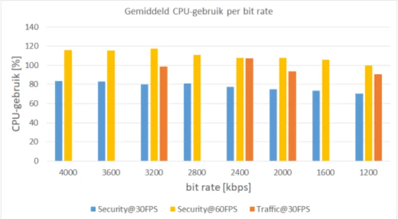
Naast de verschillende opties worden ook verschillende soorten video’s getest die als live stream kunnen binnenko-men. De eerder gebruikte verkeersbeelden worden in deze experimenten vervangen door iets rustigere beelden zoals een securitycamera aan een huis die kan filmen aan 30 of 60 frames per second, of een natuurcamera in een bos. Deze laatste heeft nog als extra eigenschap dat deze ’s nachts in-frarood beelden opneemt in plaats van in kleur te filmen. Elk experiment produceert een output van 30 frames per second.
door de CPU dan de verkeersbeelden. Dit geldt enkel als dezelfde frame rate behouden wordt: Beelden van 60 fps transcoden naar 30 fps heeft gemiddeld meer rekenkracht nodig. Dit resultaat is te zien op Figuur 2.
Fig. 2. CPU-gebruik per output bit rate.
Resultaten voor 3 verschillende video’s: de originele verkeersbeel-den en de security beelverkeersbeel-den met een frate rate van 30 en 60 frames per second.
Ook de beelden van de natuurcamera bevatten niet veel beweging en waren een lichtere last op de CPU. De nacht-beelden zijn gefilmd in grijswaarden en moeten dus geen data opslaan over de kleur van een pixel. Dit verlaagt de bit rate aanzienlijk, maar ook hier wordt weer vastgesteld dat een lagere bit rate niet betekent dat er minder CPU kracht voor nodig is. Het transcoden van de nachtbeelden produceert dezelfde resultaten als de beelden met daglicht. Ook wanneer de overgang van dag naar nacht wordt uit-getest is er geen verschil merkbaar in CPU-gebruik. Dit komt omdat het transcoding proces een vaste output bit rate instelt dat gehaald moet worden, dit overheerst het CPU-gebruik.
V. Conclusie
Deze analyse heeft verschillende manieren aangetoond waarop het CPU-gebruik van een live transcoding proces kan geoptimaliseerd worden. De opties en instellingen han-gen natuurlijk af van de context waarin het proces nodig is. Ten eerste zorgen hogere resoluties voor een hogere nood aan rekenkracht. De juiste preset of CRF waarde kiezen, die door de codec gebruikt wordt, is een afweging tussen kwaliteit van de output en de hoeveelheid CPU-gebruik. Ten slotte zijn videobeelden met minder beweging, zo-als huiselijke securitycamera’s, gemakkelijker te verwerken voor de CPU dan beelden van bijvoorbeeld een snelweg.
List of Figures 4 List of Tables 6 List of Listings 7 1 Intro 8 2 Problem Definition 10 2.1 The basics . . . 11 2.1.1 Resolution . . . 12 2.1.2 Compression . . . 13 2.1.3 Codecs . . . 16 2.1.4 Containers . . . 20 2.1.5 Video Streaming . . . 21
2.2 Live video transcoding . . . 22
2.3 Tools . . . 22
2.3.1 FFmpeg . . . 23
2.3.2 Youtube-dl . . . 23
2.3.3 MediaInfo . . . 23 1
2.3.4 Bitrate Viewer . . . 23 2.3.5 Docker . . . 24 2.3.6 Virtual Wall 2 . . . 24 3 Testing Environment 25 3.1 Original Situation . . . 25 3.1.1 Input . . . 29 3.1.2 Testing Files . . . 31 4 Experiments 35 4.1 Different Aspects . . . 35 4.1.1 CPU usage . . . 36 4.1.2 Output quality . . . 36 4.2 Experiment hierarchy . . . 39 4.3 Automation scripts . . . 41 4.3.1 Execution . . . 41
4.3.2 Compute CPU usage . . . 45
4.3.3 Compute PSNR and SSIM . . . 48
5 Results 50 5.1 Initial Experiment . . . 50
5.2 Optimizing the execution time . . . 52
5.3 Adjusting libx264 encoding options . . . 54
5.3.1 Preset values . . . 54
5.3.3 CRF values . . . 57
5.4 Multi-bitrate Output . . . 59
5.5 Other types of input . . . 60
5.5.1 Security camera . . . 60
5.5.2 Wildlife camera . . . 61
5.6 H.265 . . . 63
5.7 Overview . . . 64
6 Conclusion and future perspectives 66
Bibliography 68
A Created Scripts 70
2.1 Example of a live video transcoding process used in an objection detection
appli-cation. . . 11
2.2 I-, B-, and P-frames . . . 17
2.3 Playback artifacts when using an non-optimal IDR setting . . . 18
2.4 MediaInfo showing an mp4 container containing three different streams . . . 21
3.1 Screenshot of a traffic video . . . 32
3.2 Screenshot of a security video . . . 32
3.3 Screenshot of the cabin at daytime . . . 33
3.4 Screenshot of the cabin at nighttime . . . 34
4.1 Testing hierarchy . . . 40
4.2 Graph of the average CPU usage over time . . . 47
5.1 Objective quality results of the first experiment . . . 51
5.2 CPU results of the first experiment . . . 53
5.3 Influence of the -re option on the CPU . . . 54
5.4 Results of using the different preset options of the libx264 codec . . . 56
5.5 Results of using the ”-tune zerolatency” option of the libx264 codec . . . 57
5.6 Results of using different CRF values of the libx264 codec . . . 58 4
5.7 Results of the experiment with security video . . . 61 5.8 Influence of different wildlife videos on the CPU . . . 62 5.9 Average CPU results per second of one test for both the daytime and concatenated
videos . . . 63 5.10 CPU and bit rate comparison between the libx264 and libx265 codecs . . . 64
2.1 Raw video file sizes with an aspect ratio of 16:9, 3 bytes per pixel color depth and
24 frames per second . . . 13
2.2 H.264 Levels . . . 20
3.1 Video Files . . . 31
4.1 Example CSV file content (sizes omitted) . . . 46
4.2 Example of a CSV file with the average CPU usage per second for one test . . . 46
4.3 Example of a CSV file with the average and maximum CPU usage after 80 seconds 47 4.4 Example of the average PSNR values of a single test . . . 49
4.5 Example of the average SSIM values of a single test . . . 49
2.1 FFmpeg command for transmuxing . . . 21
3.1 Bash script that performs the transcoding process - Part 1 . . . 27
3.2 Bash script that performs the transcoding process - Part 2 . . . 28
3.3 Bash script to feed live data to the transcoding script . . . 29
4.1 Bash script that is used as entrypoint of the Docker container . . . 42
4.2 Bash script that starts the five executions for a test . . . 44 4.3 Bash script to calculate PSNR and SSIM values for each output of an experiment 48
1
Intro
The Internet of Things is a rapidly growing space. More and more devices get smarter and are connected to the Internet. In an industrial context IoT is widely used to obtain huge amounts of sensor data from machines, which is analyzed and distilled into useful metrics such as maintenance prediction, anomaly detection and performance. Imec’s City of Things project1isthe perfect example of an industrial IoT environment. The City of Things architecture consists out of huge variety of sensors, gateways and actuators, installed around the city. All these machines send their data to a main framework for processing.
One example of these machines that transfer data for processing are the CCTV cameras. These cameras produce video files 24/7 that have to be available for live monitoring and Video On Demand (VOD) services. Processing video streams require a different kind of architecture than other sensor data. Therefore, in this dissertation, the effects of video streaming in an industrial IoT context will be analyzed. Specifically, the live transcoding process that takes place at the main framework will be tested and experimented on. This process accepts its input video from multiple sources and transforms each input to an output format with certain well defined properties. The different aspects of this operation will be thoroughly inspected and tested for multiple scenarios.
As an introduction, the basics of video and video transcoding will be explained, together with 1https://www.imec-int.com/cityofthings/city-of-things-for-researchers
the tools used during the testing phase. Next the testing environment and the used video files are covered, followed by a description of the different aspects of these experiments and the automation process. In the last chapter the results of all the experiments will be discussed. This analysis will not only focus on the CCTV cameras in Antwerp, therefore the results will be applicable to most live video transcoding processes in an industrial context.
2
Problem Definition
With the current available technologies a large variety of sensor data can be obtained. The majority of these data types are still small numerical values that can be easily stored in a queue (such as Kafka1) and a time series database after being processed (such as InfluxDB2).Other data, such as video feeds from CCTV security cameras or cameras doing quality inspection in a production line, is very different and comes with a completely different set of challenges:
1. The video feeds can have wildly different encodings (AVC, HVEC, MPEG, …), resolutions (1080p, 720p, ...), bit rates and can be offered in different container formats (avi, mp4, mkv, …).
2. The throughput must be a lot higher to process video than tiny sensor values. Message based queues such as Kafka would add too much overhead.
3. Video feeds can not be easily stored in a time series database and are instead transcoded to a common format to store on disk directly. This data should be accessible in real time as live feeds and as video on demand.
As such, video feeds are not often analyzed even though they could provide useful additional 1https://kafka.apache.org/
2https://www.influxdata.com/
metrics once processed. A YOLOv33 object detector could extract objects from the feeds and
distill the video to a series of tags that is much easier to query (e.g. ‘was a person detected between 02:00 and 04:00 on the entrance camera?’). Some cloud providers, such as Amazon, have added these capabilities in their portfolio4 but not every industrial partner is keen on
uploading their sensitive data to the public cloud.
The current setup will accept video streams from CCTV cameras through an API. This API will send the received files to the buffer that feeds the transcoding process. This buffer helps when the CPU of the transcoder cannot keep up with the incoming streams. After transcoding, the DASH chunks are saved to the storage. These chunks can be used by multiple applications. One option, shown in Figure 2.1, is to use them for objection detection, together with other incoming sensor data. Another possibility is for them to be exposed through a web site for live monitoring.
Figure 2.1: Example of a live video transcoding process used in an objection detection applica-tion.
2.1 The basics
This master thesis will mainly focus on the first challenge: the wide variety of encoding and decoding options with the associated video files and their influence on the performance. To understand the process that handles the incoming live data we must first take a quick look at the basics. Video files and streams contain a lot more data than other digital files such as documents or emails. A video file consists of many still frames that should be played one after
3https://pjreddie.com/darknet/yolo/ 4https://aws.amazon.com/rekognition/
the other.
2.1.1 Resolution
Every frame, like all digital data, is made out of discrete little elements. The elements that make digital pictures appear on a screen are called pixel elements, or pixels. The number of pixels it takes to create such an image is called the resolution of a picture. To create a picture so that humans can not distinguish the individual pixels, a large resolution is needed. However, studies have shown that the amount of pixels needed to recognize objects is much lower than expected[1]. When showing people different images of with different amounts of pixels, a res-olution of only 289 pixels, or 17 by 17 size, is enough to distinguish a photo of a human face. Recognizing an outdoor scene requires a minimal resolution of 32 by 32 pixels while an indoor scene needs at least 1600 pixels in the frame, or a resolution of 40 by 40.
Because of the huge amount of pixels in these frames, resolutions are mostly expressed in height and width values. A modern TV can easily have 921.600 pixels, but the ”1280x720” represen-tation is a more comprehensible way of expressing the resolution. The higher the resolution goes, the shorter, and less accurate, the abbreviation becomes: ”3840x2160” pixels are more commonly known as a 4K resolution and ”7680×4320” as 8K. These names represent an ap-proximation of the width of the resolution.
If less than 2000 pixels can be enough to distinguish most objects, why are modern resolutions made up of millions of pixels? And why the continuous growth of resolutions on modern screens? The answer is simple: quality. The more pixels representing the object, the clearer and smoother the object looks. Before digital pictures were a thing, quality was already improving in the do-main of film. Films were recorded on film stock, a plastic strip containing light-sensitive silver halide crystals[2]. These crystals, when shortly exposed to light, can produce chemical changes in the crystals that can be developed into photographs. The size of the crystals determine the characteristics of the film, including its resolution. For a while, the Standard Definition, 720 by 480, of TV’s at home could not compete with the quality of cinema, but with the arrival of High Definition, the race for higher resolutions began.
The increase of pixels to create a picture comes with the increase of digital data to represent them. For example: a modern standard HD picture has a height of 720 lines of pixels, with an aspect ratio of 16:9 this results in a total amount of 921.600 pixels per frame. Each pixel can represent multiple colors. The most widely used color depth is True Color which uses 24 bits
or 3 bytes per pixel to represent the color of one pixel. If every pixel is represented by 3 bytes and the video file has 24 frames per second, then one second of raw video would have a size of 66.355.200 bytes or 66,36 MB. Extending this to a 30 minute video increases the file size to an excessive 119,44GB.
With the increase of screen resolutions this number will only grow bigger. If we take the same example but with a 4K resolution, 2560x1440 pixels, the size of a 30 minute video would be 477,76 GB as can be seen in Table 2.1. It is clear that streaming files of this size is impossible with the internet bandwidth of the average user. To make video streaming and many other video applications possible, compression is used.
width ∗ height ∗ bit depth ∗ f ramerate ∗ duration = f ilesize
2.1.2 Compression
Let’s say a person at home wants to watch a 30 minute video on YouTube and his bandwidth is good enough that YouTube’s Adaptive Bit Rate (ABR) algorithm selects the 1280x720 version of the video during the whole 30 minute duration[3]. The video used in this example is the 2012 Tesla Motors Documentary by National Geographic5. Using youtube-dl6 and FFmpeg7 (see
Section 2.3) to download the first 30 minutes of this documentary, the size of the downloaded file is ’only’ 149 MB. This is merely 0,12% of the raw value calculated in Table 2.1. To explain this great decrease in file size, some background information about video compression is needed.
Width Height 1 Frame[B] 1 sec [B] 30 min [GB]
426 240 306720 7361280 13,25 640 360 691200 16588800 29,86 854 480 1229760 29514240 53,13 1280 720 2764800 66355200 119,44 1920 1080 6220800 149299200 268,74 2560 1440 11059200 265420800 477,76
Table 2.1: Raw video file sizes with an aspect ratio of 16:9, 3 bytes per pixel color depth and 24 frames per second
The goal of video compression is to shrink the audio and video streams down to a smaller, more 5https://www.youtube.com/watch?v=rD9PGi8hHvY
6https://youtube-dl.org/ 7https://www.ffmpeg.org/
user-friendly size that can for example be delivered over the Internet. Reducing the size of a video file and compression in general naturally comes with a cost: loss of (sometimes unneces-sary) data. The basic idea of compression is to store the information in a file using fewer bits than the original. With this new representation the original data has to be rebuilt.
Video compression has multiple aspects. First, image compression has to be considered. Since a video consists out of many frames it seems only logical to look into how a single frame can be compressed. The compression of a digital image tries to reduce the amount of data needed to represent that image. Digital images have 3 basic data redundancies [4]:
1. Spatial redundancy or correlation between neighboring pixels.
2. Due to the correlation between different color planes or spectral bands, a spectral redun-dancy exists.
3. Due to properties of the human visual system, the psycho-visual redundancy exists. The first two redundancies occur when certain patterns form between the pixels and/or the color representations of each pixel. Similarities in the amplitudes or brightness levels of nearby pixels can form a spatial redundancy. The spectral redundancy or color redundancy is formed by correlations of the red, green and blue (RGB or YUV8) components of a pixel[5]. The
third redundancy is caused by the incapability of the human eye to recognize certain spatial frequencies. Compression can now be achieved by removing one or more of these redundancies.
Implementations
There are multiple different technologies that can be used to implement this video compression, called codecs. A codec consists of 2 main components: the enCOder, which compresses the video file and the DECoder that reconstructs the original file [6]. Most codecs follow a video coding format. These formats contain a recommendation on how to compress and decompress the video, such as the compression algorithm. One example of such format was already used in the examples above: H.264. Some of these formats, like H.264, are approved by standardization organizations such as ISO or the ITU-T9, these are called video coding standards.
Some other, less popular, video coding formats today are H.265, 4, VP8, VP9, MPEG-2 and MPEG-1[6? ]. These are not to be confused with codecs, which are specific imple-mentations of these formats. Examples of such codecs include libx264(H.264), libx265(H.265),
8https://www.pcmag.com/encyclopedia/term/55165/yuv 9https://www.itu.int/rec/T-REC-H.264
OpenH264(H.264), libvpx(VP8, VP9) and FFmpeg, which has implementations for many for-mats.
Most video files also have an associated audio file, which can also be encoded and decoded. Like video codecs, audio codecs follow audio coding formats. Examples of these formats include MP3, AAC and Opus. An audio codec is a specific software or hardware implementation that can perform the compression and decompression of the audio files according to the format. An example of an audio codec is LAME, which is one of the implementations for the MP3 standard. Many image compression techniques exists, and can be placed in two categories: Lossy or lossless compression[4].
Lossy vs Lossless
Lossless compression reduces the file size by removing data that is not needed to allow a perfect reconstruction of the original content. Lossy compression, as the name suggests, compresses the file by removing some of the information in the original representation, making this technology irreversible. Therefore lossy compression ensures a much higher compression rate than lossless, at the expense of a loss in quality. Lossless compression techniques can perform at a factor of 5 to 12, while lossy techniques can have a factor up to 100 if visible artifacts are acceptable[7].
Transform coding
The most commonly used compression techniques are based on mathematical transformations such as the Discrete Cosine Transform (DCT) or wavelet transform. DCT is considered to be the most efficient technique and is used in the JPEG format for image compression and MPEG and H.26X video codecs. In short, the DCT can describe data as a sum of cosine functions with different frequencies. In the case of JPEG compression, any block of data of 8 by 8 pixels can be represented by combining 64 different cosine functions each with their own coefficient. The 8 by 8 blocks are filled with integer values from 0 to 255 per RGB channel. These values are then transformed by the Discrete Cosine Transform function resulting in an 8 by 8 block of coefficients. The redundancy here is that the low frequency cosine waves will usually have a much bigger impact, and thus coefficient, than the high frequency ones. This means that if some high frequency waves, with low coefficients, would not be applied to reconstruct the image, the image would be very similar to the original. Using quantization tables and mathematical functions, the low coefficients can be filtered out and set to 0. This leaves only the coefficients of cosine waves that have a sufficient impact on the reconstruction. Depending on the quantization table
used, up to 90% of the 64 integers can be set to 0. After linearizing the data, a data stream that contains a lot of zeros is obtained, which is ideal to encode using Huffman coding. This entire process is mathematically reversible resulting in a very similar image, with some small artifacts.
2.1.3 Codecs
Each video codec will have its own design and implementation, but some aspects will be present in most codecs. These aspects will be covered in the following paragraphs.
I-, B-, and P-Frames
Video files are basically a lot of images placed sequentially in a file. Compressing every frame using JPEG would require a lot of CPU power and would not be very efficient. In addition, video compression has its own redundancy it can exploit: neighboring video frames usually have a lot of similarities since they will show the same object that is shifted a small amount each frame. The basic concept is that some frames are compressed using image compression, and the next frames can reference parts of this first frame that are equal, meaning they don’t have to be stored in that frame. A number of successive frames in a video stream is called a Group of Pictures or GOP. Frames in a GOP can use the other frames in that GOP for referencing. Encoders use different types of frames to establish this. Most modern codecs will use three different types[6]:
1. I-frames 2. B-frames 3. P-frames
Each one of these frames has their own function during the compression process. In the H.264 standard, the compression process uses both intra coding and predictive coding. This standard will be used in the following explanation. Later the H.265, VP8 and VP9 formats will briefly be described. An example of the different frames in a GOP is shown in Figure 2.210.
10 http://what-when-how.com/display-interfaces/the-impact-of-digital-television-and-hdtv-display-interfaces-part-2/
Figure 2.2: I-, B-, and P-frames
The consecutive frames of a video are not perfectly equal, only parts of a frame can be equal to parts of another frame. To be able to reference these parts, video frames are divided into multiple blocks called macroblocks. These macroblocks, consisting of 16x16 luma(brightness) samples instead of RGB samples, can be divided again into transform blocks and prediction blocks.
The I-frames, used for intra coding, are the first frames of every GOP, also called key frames. These frames are completely self-contained which means they have no references to other frames. The I-frames are compressed using still image compression techniques such as JPEG[4]. The key frames are also used as the starting and stopping point for a decoder. Between these points the decoding can begin and continue correctly[7]. As mentioned before, using only intra coding would result in a non optimal compression efficiency. The interval of I-frames can be specified when encoding a video file and can have an impact on the video quality as well as the resources needed.
The H.264 specification has two types of I-frames: normal I-frames and IDR-frames, or Instan-taneous Decode Refresh frames. If an IDR-frame is encountered during encoding, no P- or B-frame after the IDR-frame can reference any frame before it. This means that the decoder will clear its entire reference buffer. For video streaming, the standard is that every I-frame is an IDR-frame. This will make compression a bit less efficient but has a positive impact on the video playback, especially if the user can drag the playhead of the video back and forth[8]. If the amount of IDR-frames is too low, blockiness of the video can occur when dragging the video in
a video player, as seen in Figure 2.311. The amount of IDR-frames can, like I-frames, be easily
specified in the encoder, for example with FFmpeg using the different command line options.
Figure 2.3: Playback artifacts when using an non-optimal IDR setting
Inter coding can compress more efficiently than intra coding by predicting the values of the blocks of a frame based on the blocks of another frame. The decoder has to save these references in the reference buffer. The two options for inter coding are predictive and bi-predictive coding. P-frames, using predictive coding, can only look backwards for these redundancies. For example: if during compression the second frame, after an I-frame, is a P-frame the encoder will compare the blocks of the P-frame with those of the first key frame. If there are similarities the P-frame can reference this block, basically telling the decoder to display that block of the reference frame instead of encoding this data in the current frame.
B-frames are very similar but they can look both backward and forward to create references. This makes the B-frame the most efficient frame used in video encoding since it will find more redundancies. The downside of using B-frames is that they are harder to decode since all the referenced frames have to be buffered when playing the video. Choosing the correct size of a B-frame interval is another encoding decision that will have impact on the final bitrate, the encoders efficiency and the quality of the video file. In the H.264 specification B-frames can also be used as reference frames, like I-frames, since this can improve quality. This option is not available in other codecs such as MPEG-2.
11 https://streaminglearningcenter.com/articles/everything-you-ever-wanted-to-know-about-idr-frames-but-were-afraid-to-ask.html
Encoding Profiles
The H.264 codec comes with a lot of different configuration options, including options concerning the aforementioned frame types. The most important option to choose when encoding H.264 is the profile. Each profile defines a set of tools and functions available in H.264 that can be used by the encoder and decoder. Because not every playback device has the same CPU power, one H.264 standard for all devices would have to sacrifice a lot of quality. H.264 defines several different profiles for different applications. The 3 most popular profiles are:
1. Baseline profile - Profile with low computing cost and lower quality output.
2. Main profile - Initially the profile with average cost and quality, used for most applications. 3. High profile - Profile designed for High Definition storage and broadcast of video, now the
most widely used profile.
The effect on output quality however of these profiles are minimal: Jan Ozer calculated the peak signal-to-noise ratio (PSNR, more in Section 4.1.2) values, which is a metric for output quality, of the lowest quality frame of many different clips, each encoded with the 3 profiles. The average quality difference based on PSNR values between the baseline and high profile was only 2.73%[6]. However, these profiles should still be taken into account when encoding because not every playback device supports every profile.
In addition to these profiles, H.264 lets you also select levels. Levels place limitations on different parameters of the encoded video file, such as bit rates and resolutions. Levels are mainly used to encode video files for different mobile playback devices. Apple for example can limit the used bit rate and resolutions for video for any of their devices. They do this by setting a profile and maximum level. For example, the original iPad supports H.264 video playback for videos created with the Main profile and a level up to 3.1[9]. Table 2.2 shows some of the levels with their properties: the max bit rate of the video and an example resolution with the highest frame rate possible at that resolution.
For clarity, most of the examples with frame rates around 30 are shown, but keep in mind that most levels can encode for higher frame rates, with lower resolutions as well. As an example, the data for level 6 shows that H.264 is capable of encoding 8K video at around 30 fps but can also encode 4K resolution video at a much higher 128.9 fps without exceeding the 240.000 kbps constraint[7].
Level Max Bit Rate (kbps) resolution @ highest possible frame rate 1 64 128×96@30.9 2 2.000 352×288@30.0 3 10.000 720×480@30.0 3.1 14.000 1,280×720@30.0 4 20.000 2,048×1,024@30.0 5 135.000 2,560×1,920@30.7 6 240.000 8,192×4,320@30.2 6 240.000 3,840×2,160@128.9 Table 2.2: H.264 Levels H.265
H.265 is the successor of the H.264 codec format and will be analyzed in one of the experiments in section 5.6.
VP8/VP9
VP8 and VP9 are Google’s equivalents of the H.264 and H.265 formats. They are mostly used by YouTube and will not be further discussed in this dissertation.
2.1.4 Containers
It is now clear that most video and audio files standard PC users interact with are in some way encoded or decoded by a specific codec. It is however not common to see a H.264 or AAC file in the file explorer. The reason for this is that the files produced by the codecs are stored in containers. Containers do not specify how their data should be encoded or decoded, they only store the data and its metadata together in one file. This means that any container could wrap any kind of data, but most containers are specialized for a specific type of content. This also introduces the concept of transmuxing: because the container can hold different types of data it is easy to change the type of the container for that data. FFmpeg for example can easily convert a .mp4 file containing a H.264 encoded video file and an AAC encoded audio file to a .mov file without changing the data that is inside. This process, also called dynamic packaging, is much more CPU friendly than transcoding since the compressed data does not need to be changed. In the FFmpeg command of Listing 2.1 the input file is a mp4 container that contains a video file encoded with any possible codec. The ’-c’ option specifies the codec used for a specific
stream, here video(:v) and audio(:a). The value ’copy’ specifies that ffmpeg does not touch the compressed data and just copies it to the output file. The -f flag stands for force and forces the container of the output file. Since the extension of the output file is already specified this force flag is actually redundant but it is used in this example to emphasize the transmuxing process.
Listing 2.1: FFmpeg command for transmuxing
ffmpeg -i input_file.mp4 -c:v copy -c:a copy -f mov output_file.mov
Containers can wrap multiple encoded files such as video streams and audio streams together. This makes it possible to produce a movie in one file that contains the video stream, the audio stream and for example a subtitles stream. This can be seen using MediaInfo, as shown in Figure 2.4.
Figure 2.4: MediaInfo showing an mp4 container containing three different streams
2.1.5 Video Streaming
Jan Ozer’s definition of video streaming is ”video delivered as it’s needed” [6]. The definition of streaming in the Cambridge English Business Dictionary is more specific: ”the act of sending
sound or video to a computer, mobile phone, etc. directly from the internet so that it does not need to be downloaded and saved first”12. This is still somewhat ambiguous: what is meant by
the internet, and how is the data sent to the end users? What both definitions don’t mention is what the source of the video is and how this is stored (or produced, for live streaming). Streaming is an alternative to downloading. Like downloading, there is some kind of server that provides the video files, but when it arrives at the user it is not permanently saved to disk. Instead of waiting until the complete file is downloaded to the hard drive, the user’s machine can already play the video files while it is still being delivered. The streamed data is not very different from the data that would be downloaded, so streaming is nothing more than a delivery method.
There are many applications that are based around video streaming and each application may use a different kind of video streaming as well.
2.2 Live video transcoding
Live video transcoding is the process of changing the codec of incoming video at real time. Live transcoding is a technique that is gaining more and more attention because of new video streaming applications such as user-generated live videos. Examples are Facebook Live, YouTube Live, Twitch TV, etc. All these applications have one thing in common: Users create video content and livestream them directly to many other users via the Internet. The users that watch these video streams all have devices with different CPU power, screen resolutions and internet bandwidth. To make these kinds of services possible the generated video content has to be transcoded to multiple quality levels. The live transcoding process is expensive on both computational and networking level, requiring a well constructed architecture. Though there are some advancements that try to shift a part of the transcoding process to the receiver side[10].
2.3 Tools
In this section the tools and programs used in this dissertation will be described briefly. 12https://dictionary.cambridge.org/dictionary/english/streaming
2.3.1 FFmpeg
FFmpeg describes itself13 as a complete, cross-platform solution to record, convert and stream
audio and video. The FFmpeg framework consists of multiple technologies that can do pretty much anything that has to do with video, audio and more. The framework consists of 3 main tools: ffmpeg, ffplay and ffprobe where the first one is the command line tool used during this master thesis. The ffmpeg tool can be used for numerous applications but will be mainly used for its conversion and transcoding capabilities.
2.3.2 Youtube-dl
Another command line program that is used is youtube-dl14. This program can download videos
and live streams from many websites, including YouTube. The program is platform independent and only needs a Python interpreter to function. With youtube-dl the user can set a lot of different options regarding the video that needs to be downloaded. Examples are the codec, the container, the resolution, and many more properties of the video.
2.3.3 MediaInfo
This cross-platform program is especially useful for showing and exporting a wide array of information of a media file. It supports 29 different file formats including mp4, mov, aac, avi, etc. and every popular codec. MediaInfo15 is a handy tool to quickly look up the resolution, file
size, and bits per pixel, an important compression-related file property. The program also has an extension that shows a tooltip with some quick info about a media file while hovering over it in Windows Explorer.
2.3.4 Bitrate Viewer
Bitrate Viewer16 is a Windows-only Graphical User Interface that does exactly as the name
suggests: It shows the varying bit rate, or data rate, of a video file plotted against the timestamp. The program also calculates the average bit rate and shows this using a line, which makes it easy to locate data spikes that can cause problems in your video file.
13https://www.ffmpeg.org/ 14https://youtube-dl.org/
15https://mediaarea.net/en/MediaInfo
2.3.5 Docker
Docker containers are widely used in this project. A custom image17 is made, based from an
Ubuntu 18.04 image, to help automate the testing process, see section 4.3.1 for more info. In this image extra packages are installed: python, the latest versions of youtube-dl and FFmpeg. Using theentrypoint command in the Dockerfile of the image a script is executed every time a container is started. This script, along with the provided arguments per ’docker run’ command, starts the transmuxing and transcoding process for a specific video file.
2.3.6 Virtual Wall 2
The virtual wall18 is hosted and operated by imec’s IDLab and consists out of 2 testbeds that
can be used for research purposes. Virtual wall 2, the testbed used during this master thesis, contains 196 different nodes, categorized in 6 different categories. Each category has different hardware specifications such as CPU’s, amount of RAM and storage. Two categories with 10 nodes in total are GPU nodes with multiple nVidia graphics cards. The nodes of this virtual wall are mainly used as bare metal machines to run the docker containers that will perform the transcoding. Using the testbed, the performance will not depend on the CPU and condition of a 5-year-old laptop. In addition, all tests will have the same hardware available and multiple containers can run simultaneously.
17https://hub.docker.com/repository/docker/csurmont/converter 18https://doc.ilabt.imec.be/ilabt/virtualwall/index.html
3
Testing Environment
3.1 Original Situation
In the IoT platform developed by IDLab, the videos that are ingested are live transcoded to AVC (H.264) in the various desired qualities (1080p, 720p, 480p, …) and stored in DASH chunks using a BASH script. The DASH1 format makes it easy to live stream using Adaptive Bit Rate
(ABR), similarly to what Netflix and YouTube offer. Adaptive Bit Rate ensures that the viewer gets the best quality possible based on the available bandwidth. This quality expresses itself in the resolution of the video and its bit rate. These different qualities need to be produced beforehand and stored individually on the server. The DASH format splits the video stream into multiple segments of a certain duration that can each be sent over the Internet individually. The initial idea was to let the script run 24/7 to transcode the incoming live stream, mainly using FFmpeg for this. In the original test setup 4 AXIS camera’s[11] were used to produce the video streams. The script was deployed to the Obelisk Platform [12] created by IDLab but caused some problems due to the high CPU load. The architecture could not keep up and the buffer that was used for the ingested video was overflowing. This would reset or stop the live transcoding process. This master thesis will research the causes of this problem and analyze all
1https://www.encoding.com/mpeg-dash/
its different aspects. The different transcoding parameters, codecs and scenarios will be thor-oughly tested and evaluated.
The main use case of the project is ingesting security camera footage, more specifically IP cameras that are placed in the port of Antwerp for the City of Things project. An example of such a camera is the AXIS Q6035 PTZ Dome Network Camera2that was used during the initial
testing phase. The resolution of these cameras is in most cases 1080p or 720p with a frame rate between 24 and 30 frames per second. Different types of cameras will be used so multiple codecs have to be supported. The video stream will arrive through the Real-Time Messaging Protocol(RTMP). Because multiple codecs will arrive at the ingest point the first step is to transmux the video files to an mp4 format.
The original bash script was made by Dwight Kerkhove3 and consists of one large FFmpeg
command and some logic to convert the script arguments into FFmpeg options. The script takes multiple arguments, each argument starting with -q and followed by 3 comma-separated integers: the scale or resolution, output video bit rate and output audio bit rate. After converting these 3 arguments into their correct form they are added to the FFmpeg command as video and audio transcoding arguments. Before the actual FFmpeg command can do its job, a few variables have to be declared and filled in. On line 3 to 6 of Listing 3.1 some variables are declared that will be used to help create the DASH chunks. the duration of one DASH chunk is specified, after that a date prefix is declared that will be used in the names of all the DASH chunks. Next are two while loops that fill in the variables used as FFmpeg options in the actual command. The first while loop reads all the command line arguments that are given to the script. Every argument that starts with the option ’-q’ represents one video output stream with the specified properties. The output streams are numbered by the videoTranscodingIdx variable. When the script is executed using the parameters -q 240,400,64 -q 480,1000,64 -q 720,1500,64 for example the script will use the following ffmpeg options while transcoding:
-b:v:0 400k -filter:v:0 scale=-2:240 -b:v:1 1000k -filter:v:1 scale=-2:480 -b:v:2 1500k -filter:v:2 scale=-2:720
The second while loop does something similar with the audio streams: For every unique audio bitrate that is given as an argument it will create an audio bitrate option in FFmpeg syntax. For example: -ab:0 64k. Since there is only one bitrate is specified, ffmpeg will create one audio stream that can be combined with all video streams. In this dissertation no audio streams will
2https://www.axis.com/nl-be/products/axis-q6035 3dwight.kerkhove@ugent.be
be used, focussing entirely on the video aspect.
Listing 3.1: Bash script that performs the transcoding process - Part 1 1 #!/bin/bash
2 set -x
3 SEGMENT_DURATION=${SEGMENT_DURATION:-10} 4 # determine the current timestamp (utc) 5 dateprefix=$(date -u +%Y%m%d-%H%m%S)
6 dateprefix=${DASH_PREFIX:-${dateprefix}} 7 8 videoTranscodingArgs= 9 audioTranscodingArgs= 10 videoMapArgs= 11 audioMapArgs= 12 videoTranscodingIdx="0" 13 declare -A uniqueAudioBitrates 14 15 while [[ $# > 0 ]]; do 16 if [[ $1 == "-q" ]]; then 17 shift
18 IFS=',' read -ra qualityParts <<< "$1"
19 videoTranscodingArgs="${videoTranscodingArgs} -b:v:${videoTranscodingIdx} \ 20 ${qualityParts[1]}k -filter:v:${videoTranscodingIdx} \
21 scale=-2:${qualityParts[0]}" -ac 2 -ab ${qualityParts[2]}k" 22 videoMapArgs="${videoMapArgs} -map 0:v:0?"
23 uniqueAudioBitrates[${qualityParts[2]}]=1 24 ((videoTranscodingIdx++)) 25 shift 26 else 27 shift 28 fi 29 done 30 31 audioTranscodingIdx="0" 32 for k in ${!uniqueAudioBitrates[@]}; do
33 audioTranscodingArgs="${audioTranscodingArgs} -ab:${audioTranscodingIdx} ${k}k" 34 audioMapArgs="${audioMapArgs} -map 0:a:0?"
35 ((audioTranscodingIdx++))
After initializing the variables the ffmpeg command can be executed. Next is a brief explanation of the different ffmpeg options4 used in Listing 3.2:
• -i: input_url, can be a video file or a video stream that is piped to the script.
• -vf: alias for -filter:v, the yadif video filter selects what interlacing mode is used. Yadif stands for ’yet another deinterlacing filter’ and value 0 enables deinterlacing of the incoming video signal.
• -r: output frame rate is set to 25 frames per second. • -vcodec: sets the video codec of the output video to H.264.
• -crf: CRF is the default quality setting for x264 and x265 encoders. The default value is 23, higher values mean lower quality due to more compression. [13]
• -acodec: sets the audio codec of the output audio to AAC. • -ac: sets the number of audio channels, 2 is stereo.
• -ab: sets the audio bitrate, 64kbps is the standard for general use AAC audio. • -keyint_min: sets the minimum interval between IDR-frames, see subsection 2.1.3. • -force_key_frames: forces the I-frames(keyframes) to follow a specific interval, also see
subsection 2.1.3.
• -async and -vsync: sets the audio and video sync modes. Value ”1” enables constant frame rate by adding or dropping frames of the video stream and enables only audio correction at the start of the audio stream, and not anymore after that.
• -f: forces the output file format to be DASH chunks in this case.
• -adaptation_sets: assigns the video and audio streams to the corresponding DASH adap-tation sets.
• -seg_duration: Defines the average duration of one DASH chunk if the -use_template is enabled and -use_timeline is disabled.
• -init_seg_name: sets the name of the initialization segment per stream. • -media_seg_name: sets the naming template of a DASH chunk.
Listing 3.2: Bash script that performs the transcoding process - Part 2 4https://ffmpeg.org/documentation.html
1 ffmpeg \ 2 -i pipe:0 \ 3 -vf yadif=0 \ 4 -r 25 \ 5 -vcodec libx264 \ 6 -crf 27 -preset veryfast \ 7 -acodec aac \ 8 -ac 2 -ab 64k \ 9 -g 50 \ 10 -keyint_min 50 \
11 -force_key_frames "expr:gte(t,n_forced*${SEGMENT_DURATION})" \
12 ${audioMapArgs} \ 13 ${videoMapArgs} \ 14 ${audioTranscodingArgs} \ 15 ${videoTranscodingArgs} \ 16 -async 1 -vsync 1 \ 17 -f dash \
18 -adaptation_sets "id=0,streams=v id=1,streams=a" \
19 -seg_duration ${SEGMENT_DURATION} \
20 -use_template 1 \
21 -use_timeline 0 \
22 -init_seg_name init-\$RepresentationID\$.mp4 \
23 -media_seg_name ${dateprefix}-\$RepresentationID\$-\$Number\$.mp4 \
24 ${DASH_FOLDER}/live.mpd 3.1.1 Input
This FFmpeg command gets its input from pipe:0, which means another process has to pipe its output into this process for it to work. The way this is done is by executing another bash script that selects input video streams, from either local or online storage and pipes it to the transcoding script. To imitate the incoming data from security cameras, youtube-dl can be used to ingest a live stream of, for example, a security camera in Banff national park, Canada5. This
is an example of a YouTube live stream that is always online. An example script can be seen in Listing 3.3.
Listing 3.3: Bash script to feed live data to the transcoding script 1 #!/bin/bash
2 set -x
3 (( $# == 4)) || { echo "Not enough arguments: link, q1, q2, q3" >&2 ; exit 1 ; } 4 link=$1 5 q1=$2 6 q2=$3 7 q3=$4 8
9 export DASH_FOLDER=LiveData 10 mkdir $DASH_FOLDER
11
12 ffmpeg \
13 -hide_banner \
14 -nostdin \
15 -i $(youtube-dl -f 'bestvideo[ext=mp4]/mp4' -g $link | head -n 1) \
16 -c:v copy -c:a copy -strict -2 \
17 -f mp4 \
18 -movflags frag_keyframe+empty_moov+default_base_moof pipe:1 2> /dev/null | \
19 ./chunk_generator.sh -q $q1,$q2,$q3
This script uses both FFmpeg and youtube-dl to convert the input data to the right format for the transcoding process. The youtube-dl command provides the location of the live data on Google’s servers. FFmpeg can retrieve this data and transmux it to an mp4 format. The ’-c:v’ and ’-c:a’ options specify the codecs used for video and audio. Since this FFmpeg command is only used to provide the input for the transcoding process, these are set to copy. This makes this process very light on the CPU and should not have a big influence on the performance. The impact will however still be tested later in Chapter 5. The output of this FFmpeg command is piped in mp4 format to the transcoding script: here it is called chunk_generator.sh. Since the mp4 format is normally a single file, the video has to be split up in fragments. That is why the ’-movflags’ option is used. It cuts the incoming mp4 files into fragments that start with every keyframe(I-frame). More information about these options can be found in the FFmpeg Formats Documentation6.
For the main part of the experiments, local storage video files will be used for testing. This is to exclude some aspects of the process that are hard to control such as the availability of the live video, or the content itself. To ingest these files a very similar script can be used that only requires FFmpeg. Instead of inserting a youtube-dl command after the ’-i’ option, a local file can be specified. This file will be piped to the transcoding script in exactly the same way.
3.1.2 Testing Files
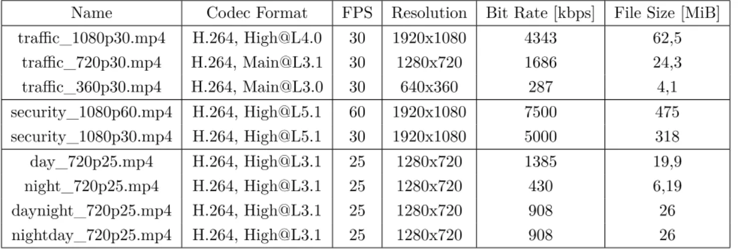
On the virtual wall there is a base folder, mounted as an NFS share, containing all the test videos. This network storage had no influence on the testing process, the same results were found when the files were copied to the hard disks of the nodes. All videos used during the experiments have a length of two minutes, except for the last pair of videos. A duration of two minutes is enough to complete the startup of the transcoding process, and is not too long, keeping the storage overhead at a minimum. In the following table all of the used video files will be covered, together with some of their properties:
Name Codec Format FPS Resolution Bit Rate [kbps] File Size [MiB] traffic_1080p30.mp4 H.264, High@L4.0 30 1920x1080 4343 62,5 traffic_720p30.mp4 H.264, Main@L3.1 30 1280x720 1686 24,3 traffic_360p30.mp4 H.264, Main@L3.0 30 640x360 287 4,1 security_1080p60.mp4 H.264, High@L5.1 60 1920x1080 7500 475 security_1080p30.mp4 H.264, High@L5.1 30 1920x1080 5000 318 day_720p25.mp4 H.264, High@L3.1 25 1280x720 1385 19,9 night_720p25.mp4 H.264, High@L3.1 25 1280x720 430 6,19 daynight_720p25.mp4 H.264, High@L3.1 25 1280x720 908 26 nightday_720p25.mp4 H.264, High@L3.1 25 1280x720 908 26
Table 3.1: Video Files
The first three files are video footage from a traffic camera that records bypassing traffic on a highway ramp. This type of video has a lot of movement and will typically be harder to encode. The camera is immobile so the trees and the grass around the road are still relatively stationary. A screenshot of the video can be seen in Figure 3.1.
Figure 3.1: Screenshot of a traffic video
Since these files contain a lot of movement, another type of video was needed to simulate a more stationary environment, such as a security camera on a driveway, or a container port dock. The next type of files simulates a security camera that is attached to a house. The camera points to the driveway and the street. The house is located in a calm neighborhood so hardly any cars pass in comparison with the traffic video. A screenshot of this type of video is shown in Figure 3.2.
Figure 3.2: Screenshot of a security video
Now the tests can be executed using video with either lots of movement or barely any movement. Another type of video that will be tested is infrared footage. Some security cameras will switch to infrared mode when it is too dark outside. This makes it easier to distinguish objects and
persons at night. Infrared footage has different properties than daylight footage. To test this, four different video files of a wildlife cam from Maryland, USA7 are used. The camera is
posi-tioned at a cabin in the forest that provides wildlife in the area with some food bowls. At night, an IR illuminator shines infrared light at the environment that bounces back to the camera. The same camera that captures the daylight video can now capture the 850nm light rays8. The
footage is also mainly stationary, with the occasional deer or squirrel entering the frame. The advantage of this camera is that it switches to infrared vision at night. Therefore the day and night clips have approximately the same content. An example can be seen in Figures 3.3 and 3.4. The last two clips in the table are a concatenation of the day and night clips, to test the effect of the transition from daylight video to infrared and vice-versa. These clips are thus the only ones with a duration of four minutes.
Figure 3.3: Screenshot of the cabin at daytime
7https://www.youtube.com/channel/UCjdVnr1eXgAV-8NKE0Yl7kQ
4
Experiments
With all these video files, their respective properties and the different encoding possibilities a well defined roadmap is needed to analyze the different aspects of the transcoding process. Every experiment should follow this roadmap so that its results can be easily compared to those of the other experiments. It is also crucial that in each experiment only one parameter of the process is changed in comparison with the other experiments. In this chapter the different aspects of the experiments will be explained, followed by a lineup of all the automation scripts that facilitate the execution of the experiments.4.1 Different Aspects
Every experiment consists of the same aspects, but some experiments will focus more on a specific aspect. In the first few experiments for example the focus will be mainly on the output quality, so the CPU usage or file size will not be relevant. This does not mean these aspects will not be calculated or saved. They can be useful in a later stage to compare to the other experiments.
4.1.1 CPU usage
The amount of CPU power that is used during the transcoding process is one of the key as-pects of this analysis. The architecture that handles the transcoding process will receive video feeds from multiple cameras. All this data will have to be transcoded at real-time to be able to create the DASH chunks quick enough to offer a multi-bitrate livestream on a web server. If the CPU cannot keep up, the incoming data will be temporarily stored in a buffer. This is useful for situations where there is a sudden change of scenery and the frames become much harder to transcode. These frames will be stored in the buffer and when the footage changes to a normal scene again the CPU can catch up, processing the incoming frames and those in the buffer quicker than real time.
If however the normal CPU usage is too high, this buffer will fill up and incoming frames will be dropped, or the transcoding process will reset, depending on the implementation. This is why it is important to monitor the CPU during all experiments.
4.1.2 Output quality
Another important aspect of the process is the visual quality of the produced output. If the main goal was to only minimize the effect on the CPU then the quality of the produced video files or DASH chunks would be unacceptable. The video would show all kinds of artifacts such as blockiness and choppiness. Blockiness is when groups of pixels, mostly in rectangular forms, are displaying the same color. Choppiness on the other hand is caused by frames being dropped, which results in stuttering or out of sync video. These effects can be caused by the transcoding process, but can also be present in the source video. When this is the case, the transcoding process can not be blamed for these artifacts.
Blockiness and choppiness are two examples of visual artifacts, that can be seen by the hu-man eye. There are multiple ways to measure the visual quality of a video. The most accurate would be to show the video to an audience in optimal circumstances. Afterwards the partici-pants would have to rate the video files. With this data the Mean Opinion Score (MOS) could be calculated[14].
Since there will be many experiments, each with multiple output files it is not practical to check every file visually. This is why another method is used to measure the video quality: objective quality metrics. These metrics can be calculated by a computer and don’t need human interac-tion. These metrics are proven to have similar results compared to the MOS[15]. This justifies their use for this purpose.