Disjunctive arcs and resource flows in project networks

(1)

DISJUNCTIVE ARCS AND RESOURCE

FLOWS IN PROJECT NETWORKS

Aantal woorden / Word count: 22.335

Sophie Laseure

Stamnummer / student number: 01505803

Promotor / supervisor: Prof. Dr. Mario Vanhoucke

Masterproef voorgedragen tot het bekomen van de graad van:

Master’s Dissertation submitted to obtain the degree of:

Master in Business Engineering: Operations Management

(2)

(3)

Confidentiality Agreement

PERMISSION

I declare that the content of this Master’s Dissertation may be consulted and/or reproduced, provided that the source is referenced.

(4)

Foreword

I would like to thank Rob Van Eynde who provided me with the necessary literature, feedback, and insightful remarks throughout the creation of this master dissertation. He set out great guidelines for this research and was very eager to provide help where needed.

Furthermore, I would like to express my gratitude to my friends and family for their moral support during the writing of this master dissertation. In particular, I want to thank Karlien Claus for her continued support and encouragement throughout this research. Also, I would like to thank Timothy De Moor for providing a different perspective on this master dissertation, and for the moral support during the entirety of my academic career at Ghent University.

(5)

List of Abbreviations

D

DG Disjunctive Graph. G

GA Genetic Algorithm.

GRPW Greatest Rank Positional Weight. J

JSSP Job Shop Scheduling Problem. L

LFT Latest Finishing Time. M

MSLK Minimum Slack. MTS Most Total Successors. N

NP-hard Non-Deterministic Polynomial-Time Hard. P

PSGS Parallel Scheduling Generation Scheme. R

RCPS Resource Constrainted Project SCheduling.

RCPSP Resource Constrainted Project Scheduling Problem. S

SA Simulated Annealing.

SSGS Serial Scheduling Generation Scheme. T

(9)

List of Symbols

A

A set of precedence constraints.

abf bf.

Ai activity i.

B

b arc index: b ∈ [1, B].

B number of edges that become arcs. C

c clique index: c ∈ [1, x]. Cn complete set.

CLc clique c.

CPp critical path activity p.

D

di duration of activity i.

d0_i0 duration of node i0.

Dn decision set.

E

E set of operations in conflict with each other. eqg edge qg.

EA eligible activities.

EF Ti earliest finishing time of activity i.

F

f arc position index: f ∈ [1, 2]. F initialization parameter. F Ti finishing time of activity i.

G

g edge position index: g ∈ [1, 2]. G directed graph.

H

H number of activities on the critical path. I

i activity index i: i ∈ [1,I]. I number of activities in a project. i0 node index i0: i0 ∈ [1, I0_].

I0 number of nodes in a project. J

j job index: j ∈ [1,n].

J maximum stage number SSGS.

Jj job j.

K

k resource index: k ∈ [1,K]. K number of resource types. L

LF Ti latest finishing time of activity i.

lj number of operations in job j.

M

m machine index: m ∈ [1,x].

Mm machine m.

M N maximum node.

M S makespan of the project. M S∗ duration of the critical path. M V maximum value.

(10)

N

n number of jobs in a job shop scheduling problem.

N number of iterations. Ni0 node i’.

N M V new maximum value. O

o operation index: o ∈ [1,Lj].

Oo operation o.

Oomj operation o belongs to job j and needs to be

processed by machine m. P

p critical path index: p ∈ [1, H]. Pi set of predecessors of activity i.

P Dy_i0 predecessor x of node i0.

Q

q edge index: q ∈ [1, Q]. Q number of edges in a project. R

r random number: r ∈ [0, 1].

Rik the number of units activity i needs of

re-source type k per time unit t.

R_i00_k the number of units node i0needs of resource

type k per time unit t. Rk resource k.

RAk the maximum number of available units of

resource type k per time unit t.

RAkt the remaining number of available units of

resource type k in time period t. S

S a feasible schedule. S0 a new feasible schedule.

S* a new optimal feasible schedule. Sn scheduled set.

sn stage number SSGS. SSy_i0 successor y of node i0.

STi start time of activity i.

T

t time unit t.

V

V set of vertices corresponding to the opera-tions.

vi priority value of activity i.

X

x number of machines.

xi0 predecessor index x_i0: x_i0 ∈ [1,X_i0].

Xi0 number of predecessors of node i0.

Y

yi0 successor index y_i0: y_i0 ∈ [1,Y_i0].

(11)

List of Tables

7.1 Structure input file. . . 28

7.2 Example "after" Variable. . . 30

7.3 Structure output file. . . 41

7.4 Example output file. . . 41

8.1 Output file of the example. . . 45

10.1 Trials SA - 15. . . 53 10.2 Trials SA - 138 projects. . . 53 10.3 Trials SA. . . 54 10.4 Trials TS. . . 55 11.1 Summary B. . . 61 11.2 Summary SA. . . 63 11.3 Summary TS. . . 64

11.4 Summary all versions. . . 65

11.5 Comparison analysis. . . 65

11.6 Summary combination. . . 66

11.7 Summary runs basic version. . . 67

11.8 Summary runs SA version. . . 67

11.9 Summary runs TS version. . . 68

11.101.000 runs B. . . 69

11.1110.000 runs SA. . . 69

11.1250.000 runs TS. . . 69

11.13Comparison PSGS vs. DG. . . 73

(12)

List of Figures

3.1 Example representation of JSSP . . . 6

3.2 Example representation of RCPSP . . . 6

4.1 Project network diagram of 8 activities . . . 8

4.2 Project schedule using SSGS . . . 8

4.3 Project schedule using PSGS . . . 9

4.4 Diversification strategy . . . 11

4.5 Intensification strategy . . . 11

4.6 Flowchart of the SSGS pseudocode . . . 13

4.7 Flowchart of the PSGS pseudocode . . . 14

4.8 Algorithm Multi-Pass Heuristic . . . 15

5.1 Example DG for Job Shop Scheduling . . . 17

5.2 Clique with 4 operations . . . 18

5.3 Job Shop Critical Path - 1 . . . 18

5.6 Job Shop Schedule . . . 19

6.1 Example Job Shop to RCPS . . . 21

6.2 Example Network Diagram for RCPSP . . . 22

6.3 Digraph - Simplification 1 . . . 23

6.4 Simplification 1 - Solution . . . 23

6.5 Problem 1 - Schedule A . . . 24

6.6 Problem 1 - Schedule B . . . 24

6.7 Problem 2 - Situation A - Network Diagram . . . 24

6.8 Schedule A . . . 25 6.9 Partial Schedule B . . . 25 6.10 Schedule B (Insertion) . . . 25 6.11 Schedule Solution A. . . 26 6.12 Schedule Solution B. . . 26 7.1 Overview Algorithm . . . 29

(13)

8.1 Example Project with 20 Activities and 2 Resource Types . . . 42

8.2 Edges of the example. . . 42

8.3 Arcs of the example. . . 43

8.4 Critical Path of the example. . . 43

8.5 Partial Schedule R1. . . 43

8.6 Partial Schedule R2. . . 44

8.7 Full Schedule R1. . . 44

8.8 Full Schedule R2. . . 44

9.1 p throughout the iterations. . . 48

9.2 p throughout the iterations adjusted. . . 48

9.3 Makespan of SA schedules. . . 48

9.4 Makespan of SA* schedules. . . 48

9.5 Initial solutions of SA schedules. . . 49

9.6 Initial solutions of SA* schedules. . . 49

9.7 Makespan of TS schedules. . . 51

9.8 Makespan of TS* schedules. . . 51

11.1 Duration of the critical path vs. actual makespan. . . 58

11.2 Duration of the critical path vs. actual makespan with restriction. . . 59

11.3 Efficiency B. . . 61 11.4 Quality B. . . 61 11.5 Duration B. . . 61 11.6 Cost B. . . 61 11.7 Efficiency SA. . . 62 11.8 Quality SA. . . 62 11.9 Duration SA. . . 63 11.10Cost SA. . . 63 11.11Efficiency TS. . . 64 11.12Quality TS. . . 64 11.13Duration TS. . . 64 11.14Cost TS. . . 64

11.151000 runs of basic version. . . 67

11.161000 runs of SA version. . . 67 11.171000 runs of TS version. . . 68 11.181.000 runs B. . . 68 11.1910.000 runs SA. . . 68 11.2050.000 runs TS. . . 68 11.21Edges - Efficiency B. . . 69

11.22Edges - Efficiency SA. . . 69

11.23Edges - Efficiency TS. . . 69

11.24Edges - Quality B. . . 70

11.25Edges - Quality SA. . . 70

(14)

11.27Edges - Duration B. . . 70

11.28Edges - Duration SA. . . 70

11.29Edges - Duration TS. . . 70

11.30Edges - Cost B. . . 71

11.31Edges - Cost SA. . . 71

11.32Edges - Cost TS. . . 71

11.33Edges - Best version. . . 72

11.34Resource constraint - Edges. . . 72

11.35Quality PSGS vs. DG. . . 72

11.36Cost PSGS vs. DG. . . 72

11.37Adjusted quality PSGS vs. DG. . . 73

(15)

List of Algorithms

1 Calculate edges . . . 31

2 Calculate arcs . . . 32

3 Calculate LFT . . . 33

4 Create critical path . . . 34

5 Create priority rule . . . 34

6 Schedule activities . . . 35

7 Schedule critical activities . . . 35

8 Calculate EST . . . 36

9 Calculate Remaining Available Resources . . . 36

10 Schedule remaining activities . . . 37

11 Calculate P AT St . . . 38

12 Find the best activity to schedule . . . 39

13 Schedule activity . . . 40

14 Simulated annealing. . . 46

15 Simulated annealing adjusted. . . 47

16 Tabu search. . . 49

17 Tabu search*. . . 51

18 Adjust R2t . . . 59

19 Insert node . . . 59

(16)

Part I

(17)

1 |

Definition of the problem

The "project scheduling problem" is the problem of constructing a schedule where each activity is allocated to a specific start time. This assignment has to be done as efficiently as possible to achieve a target objective. These activities are tasks that have to be completed for the project to finish. The target objective can be a due date by which the project needs to be finished, or a budget that cannot be exceeded,... To be feasible, a schedule needs to respect two types of constraints; precedence constraints and resource constraints. The precedence constraints enforce that a certain activity cannot start before all its predecessors are completed. Additionally, there are renewable resource constraints that indicate the specific amount of resources needed during each period of the duration of the activity. These resources are the means that the different activities require for completion. The fact that they are renewable means that one unit can be used several times, however, not at the same time. One activity may require several types of resource, and several units per type of resource. The types of resources can vary from money to people, to equipment, to machines, ... Furthermore, resources are scarce, which means that there are only a limited amount of them available for each project. At each time unit, the amount of used resources needs to be lower than the limited amount of available resources for the project.

Activities can be scheduled in series, in parallel, or in a combination of both. When activities are scheduled in series, they occur in a linear pathway where one activity happens in consequence with another. The first activity has to be finished for the second activity to be able to commence. There is only one activity being executed per time unit. On the other hand, when activities are scheduled in parallel, different activities can be executed at the same time unit. As stated earlier, each activity requires a certain amount of resources. When parallel activities require the same resources, a conflict occurs if the available amount of resources is not high enough. Because resources are scarce, activities may need to be postponed until the necessary amount of resources becomes available (Kolisch, 1996b).

Different approaches can be used for deciding which activities need to be postponed, and which have to be executed as soon as possible. Some examples are priority rule-based scheduling, meta-heuristics, ... These meth-ods, priority rule-based scheduling and meta-heuristics, have already been thoroughly researched. A proposed approach for solving the Resource Constrainted Project Scheduling Problem (RCPSP), that has not received quite as much attention in the aforementioned research, is the Disjunctive Graph (DG) model. Therefore it is this approach that will function as the main focus of this master dissertation. The DG method is a well-established model used for solving the Job Shop Scheduling Problem (JSSP). The JSSP is similar to the RCPSP, but the problem is less complex. There is only one resource unit per type of resource available and each task needs only one resource type per time unit. Due to the limited resource availability, tasks that need the same resource type can only be scheduled in series, not in parallel.

(18)

2 |

Research approach

This master dissertation is divided into four main parts;

– Part 1 : Introduction – Part 2 : Literature review – Part 3 : Methodology

– Part 4 : Results and conclusion

The first part of the master dissertation is the definition of the problem (Section 1). Followed by explaining the structure of the research approach (Section 2).

The second part of the research is an overview of the existing literature on this topic. The main topic of this master dissertation is the disjunctive graph (DG). However, to get some context and inspiration for solving the problem, there will also be some similar topics discussed. The DG is a solution method used for the Job Shop Scheduling Problem (JSSP). So, to fully understand the DG method, the JSSP is explained (Section 3.1). The objective of this master dissertation is to apply the DG method on the Resource-Constrained Project Scheduling Problem (RCPSP). So, next to the JSSP, the RCPSP will also be illustrated (Section 3.2). Next to these scheduling problems, several solution approaches for the RCPSP will also be discussed (Section 4). The discussion of these solution approaches is aimed at gaining insight into how the RCPSP can be solved with the use of the DG method. Lastly, the use of the DG method for the JSSP will also be fully researched (Section 5). This is a general review of the existing literature about the DG.

The third part of the master dissertation is the used methodology. The first objective of this master disser-tation is to show how the DG method solves the JSSP, this is done in the second part. The second objective is to investigate how this DG method may help to create project schedules and to design a scheduling method that works for the RCPSP. The idea is to identify the problems and differences that come along with using the DG for solving the RCPSP (Section 6). For each problem that arises, one or more potential solutions/simplifications are discussed so that implementation is attainable. When all problems have found an applicable solution, all so-lutions are combined in a basic algorithm that solves the RCPS with the use of the DG (Section 7). An example of the found solution approach will also be illustrated (Section 8). Afterward, the basic algorithm is extended with meta-heuristics to create different versions of the algorithm (Section 9). Each version of the algorithm is optimized to its fullest potential (Section 10).

The fourth, and last, part of the research is the analysis of the different found versions of the algorithm. The results of the different versions of the algorithm are analyzed and compared with one another, and with an already well-established scheduling method (Section 11). Lastly, a conclusion is drawn on the question if the

(19)

Part II

(20)

3 |

Scheduling Problems

Firstly, an overview of the terminology is given. Since this topic finds its roots in manufacturing, the vocabulary related to scheduling is derived from that industry. A scheduling problem refers to a set of activities that need to be executed while maximizing or minimizing an objective function. An activity is a processing step of a certain project. Each activity has a specific duration and a certain amount of resources needed to complete the activity. Resources can be machines, tools, manpower,. . . The makespan of a project is the duration from start to finish (Fortemps & Hapke, 1997). Scheduling problems can also be referred to as being "Non-Deterministic Polynomial-Time Hard (NP-hard)". This means that there is no exact polynomial-time algorithm that can solve the problem unless the polynomial-time equals the non-deterministic polynomial-time, i.e. the time to find a solution grows exponentially with problem size (Garey & Johnson, 1979).

3.1 The Job Shop Scheduling Problem

“Job Shop Scheduling Problem (JSSP)” can be defined as an optimization problem where a set of jobs J (n = amount of jobs) consist of a set of operations O (lj = amount of operations for job j) and these operations need

to be assigned to a set of machines M (x = amount of machines) at particular times. When talking about a specific job, operation, or machine, the indices used are j, o, and m. The makespan need to be minimized by scheduling the operations on the machines in the most optimal way. The makespan is the finishing time of the last scheduled activity. A job is a sequence of operations. These operations have to be processed in a specific sequence to finish the job i.e. each operation has precedence constraints that determine the order in which they visit each machine to complete the job. Each operation has thus two characteristics; the duration of the operation and the machine that needs to process the operation. The duration of the operation is the time the machine needs to finish the operation. There are two important limitations. The first limitation is that no two jobs can be processed at the same time by the same machine, i.e. when two operations need to be processed by the same machine one operation has to wait until the other operation is finished processing. The second being that no job can be executed at the same time by two different machines, i.e. one machine will have to process the job before the job can move on to the next machine. (Gromicho et al., 2012).

JSSP are often illustrated by a network diagram. Each node of the network diagram represents an operation. And each sequence of nodes and thus operations portrays a job. Inside each node (operation) is an indication of the machine on which the operation needs to be processed and of the job to which the operation belongs. This indication is typically Oomj where the subscript o represent the operation, m the machine, and the subscript j the

job. When an operation has one subscript, the subscript represents the operation number. When an operation has three subscripts, they represent the operation, the machine, and the job. An example of this representation

(21)

J2 of 2 operations O122and O212. In total there are 2 operations that need to be processed by M1, 2 operations

by M2 and 1 operation by M3.

Figure 3.1: Example representation of JSSP

3.2 The Resource Constrained Project Scheduling Problem

"The Resource Constrainted Project Scheduling Problem (RCPSP)“ is a generalization of the Job Shop Schedul-ing Problem. The activities from the RCPSP can be compared to the operations from the JSSP. A project consists of I activities. A specific activity gets symbolized as Ai where i is the activity index. Each activity has

a certain duration (di) until their completion and they need some kind of resource. There are K resources in

a project. RAk represents the number of available units of resource type k per time unit. Rik represents the

number of units of resource type k activity i needs per time unit to be processed. The resources used with the JSSP are machines. The RCPSP is more general because there can be more than one unit of each material. The availability of a specific resource can be equal to one (like in the JSSP), but the limit may be higher.

Another similarity between the RCPSP and the JSSP is the resemblance of the representation of the problem. All activities are portrayed with a node. In the right upper corner of each node is an indication of the duration of the activity. And in the right lower corner an indication of the number of units needed for the execution of the activity. This can be more than one kind of resource. The precedence constraints are illustrated by the arcs between the activities. When there is an arc between A1 and A2 (A1→ A2), it means that activity 1 must be

finished before activity 2 can be initiated. The project starts at the node with a 0 indication and the ∞ node. An example of the general representation of the RCPSP is shown in Figure 3.2.

(22)

4 |

Solution Approaches for the RCPSP

4.1 Priority Rule Based Scheduling

Priority rule-based scheduling consists of two components; a priority rule and a schedule generation scheme. The priority rule determines the order in which the activities are selected. Once an activity is selected it can be scheduled according to the chosen scheduling generation scheme (Kolisch, 1996b).

4.1.1 Schedule Generation Scheme

The two most important schemes of priority rule-based scheduling are Serial Scheduling Generation Scheme (SSGS) and Parallel Scheduling Generation Scheme (PSGS). These methods produce feasible schedules by ex-tending a partial schedule in a stage-wise fashion. In the partial schedule a subset of the activities has already been scheduled. Both scheduling schemes derive feasible schedules since both methods respect the precedence and resource constraints (Kolisch, 1996b).

4.1.1.1 Serial Schedule Generation Scheme

In the SSGS, the next activity is selected at each stage from the priority list. The chosen activity is then scheduled as soon as possible without violating either the precedence or the resource constraints. As proven by R. Kolisch, a schedule developed with the SSGS and any priority rule belongs to the set of active schedules (Kolisch, 1996b). An active schedule is a feasible schedule where no activities can be locally or globally left-shifted (Sprecher et al., 1995).

Locally or globally left-shifted can be explained as follows. From a feasible schedule S = (F T1, . . . F Ti, . . .

F Ti), activity i is selected and assigned the earliest finish time EF Ti. This action that replaces F Ti with EF Ti

is called “left shifting”. This action of left shifting is referred to as a local left shift of activity i, if the resulting schedule and all intermediate schedules are feasible. However, when the resulting schedule is feasible but at least one intermediate schedule is infeasible, the left shift is a global left shift of activity i (Sprecher et al., 1995).

The procedure is illustrated in Figure 4.6 below. An iteration is performed to schedule the project. There is a stage number sn which represents the iterations of the algorithm. There are two sets of activities, scheduled set Ssn and decision set Dsn. Scheduled set Ssn contains the activities that already have been scheduled. This

means that Ssn represents the partial schedule. Decision set Dsn are the unscheduled activities of which the

predecessors are in the scheduled set Ssn. The first step in the flowchart is the initialization of the procedure.

The stage number sn is set to 1 and the scheduled set Ssn is defined as being empty. After the initialization,

the iteration is introduced. As long as the number of activities in the scheduled set Ssn is strictly smaller than

(23)

RAktrepresents the leftover capacity of the renewable resource k in period t. After that, the next activity i∗ is

selected based on the priority value vi of each activity. Next, the earliest precedence feasible finish time EF Ti

and the latest precedence feasible finish time LF Ti are computed. The last steps are defining the scheduled

set Ssn+1 of the next stage and specifying the next stage n + 1. So set S2 contains the activities that already

have been scheduled when the second iteration start. If the number of activities in the scheduled set Ssn is still

smaller than stage number J , than the iteration is repeated. If this is not the case, the procedure is stopped and all the activities are scheduled (Kelley, 1963).

Example 1. A project of 8 activities needs to be scheduled. There is a priority list = (1,3,4,2,7,5,6,8) and a resource constraint of 6. This example is illustrated with the network diagram shown in Figure 4.1. The project schedule using a SSGS is represented on Figure 4.2.

Figure 4.1: Project network diagram of 8

ac-tivities Figure 4.2: Project schedule using SSGS

4.1.1.2 Parallel Schedule Generation Scheme

There are two algorithms called the parallel method: The algorithm of Brooks (Bedworth & Bailey, 1987) and the algorithm of Kelley (Kelley, 1963). Most literature uses the scheme presented by Brooks, so the same will be used here. The PSGS iterates over the time horizon of the project, in contrast to the SSGS which iterates over the priority list. At each decision point, it determines which activities are eligible. The eligible activities (EA) will then be scheduled in order of the priority list. When the starting time of the activity equals the decision point, the activity is scheduled. If the resource constraints do not allow this allocation, the activity is incremented to the next decision point. As proven by R. Kolisch, a schedule developed with the PSGS and any priority rule belongs to the set of the non-delay schedules (Kolisch, 1996b). A non-delay schedule is a feasible schedule where none of the sub-activities of the corresponding unit-time-duration schedule (a schedule where each activity is split into sub-activities with duration ”1”) can be locally or globally left-shifted (Sprecher et al., 1995). In Figure 4.7 below, the pseudocode is shown. The SSGS had two sets of activities, the scheduled set Ssn and the decision set Dsn. The PSGS has 3 sets of activities, the decision set Dsn, the active set Asnand the

complete set Csn. Here the decision set Dsn has a different use than in the serial schedule generation scheme.

The decision set Dsn contains all unscheduled activities that can be scheduled. Meaning that they are allowed

(24)

Example 2. The same project instance is used as in Example 1, but this time the PSGS is used instead of the SSGS. The project schedule using a PSGS is represented on Figure 4.3.

Figure 4.3: Project schedule using PSGS

4.1.2 Priority rules

The priority rules determine in which way activities are selected. There are four main approaches for classi-fying priority rules. A first distinction can be made between network, time, and resource-based priority rules (Lawrence, 1985; Alvarez-valdes & Tamarit, 1989). The second distinction is the division of priority rules into static and dynamic priority rules. Static priority rules are those that return the same priority value for a certain activity. Dynamic priority rules, on the other hand, may return different values depending on the decision point of the algorithm. A third distinction is made based on the amount of information processed. When there is a lot of processed information, a priority rule is referred to as global. If this is not the case, the term local priority rules is used. The last distinction is about the use or lack of use of a lower bound. Meaning that there are priority rules where the priority value is a lower bound or where the priority rule makes use of a lower bound on one side, and priority rules where this is not the case (Kolisch, 1996b).

4.1.3 Performance Overview

Extensive research has been done concerning the performance of various priority rules. Kolisch (1996a) analyzed four different studies about the performance of the classical priority rules. These four reviews were compiled by Davis & Patterson (1975), Alvarez-valdes & Tamarit (1989), Valls et al. (1992), and Boctor (1990). These reviews show that the best classical priority rules are Most Total Successors (MTS), Greatest Rank Positional Weight (GRPW), Latest Finishing Time (LFT), and Minimum Slack (MSLK). When assessing performance of these different priority rules, it can be concluded that the MSLK priority rule that has a superior performance, followed by the GRPW and LFT priority rules, and lastly the MTS priority rule. Davis & Patterson (1975), Boctor (1990), and Valls et al. (1992) prove that the MSLK priority rule has the best performance out of their researched priority rules. Alvarez-valdes & Tamarit (1989) concludes that the GRPW priority rule has a superior performance than the LFT priority rule, and that the LFT priority rule has a superior performance than the MTS priority rule. However, when using the Parallel Scheduling Generation Scheme (PSGS), the MSLK and the LFT priority rules are equal. This equality has been demonstrated by Davis & Patterson (1975). The use of the LFT priority rule will be preferred above the MSLK priority rule, when using the PSGS, due to its easy calculation (Kolisch, 1996a).

(25)

4.1.4 Evaluation

4.1.4.1 Advantages

Priority rule-based methods have several advantages. To start, priority rules are fast regarding the computational effort (Storer et al., 1992; Leon & Balakrishnan, 1995). Furthermore they are very intuitive and robust, which makes them easy to understand and to explain to others who may have less knowledge about the subject. A last big advantage of priority rule-based scheduling is that they can be self-decided. Users can decide to make their own priority rule for the benefit of the project. Supervisors are expected to know their projects and therefore understand what priority rule positively influences their outcome (Kolisch, 1996b).

4.1.4.2 Disadvantages

There are also disadvantages to the priority rule-based methods. One of them being that there is no way to know if the found solution is the optimal solution. Different rules result in different schedules. And by comparing them the best fitting schedule can be selected. However, this method offers no certainty that the chosen solution is the optimal solution. Another disadvantage is that you do not know in advance which priority rule will result in the best schedule. There is not one priority rule that always results in the best schedule for different projects. Different rules will be optimal for different projects depending on the characteristics of that project. So when generating the best schedule for a project, it is recommended to apply several priority rules.

4.2 Meta-Heuristics

Another way to solve the RCPSP is via meta-heuristics. They are part of the heuristics-family. As shown by Blazewicz et al. (1983), the RCPSP is NP-hard. Until now, it appears that the best exact methods can only find solutions for instances involving at most 60 activities where the instances are not highly-resource constrained (Pellerin et al., 2020). The goal of exact methods is to obtain the optimal feasible solution for the scheduling problem. Because of this they are limited to small projects under strict assumptions (Vanhoucke, 2012). However, in practice, most realistic projects exceed 60 activities. In these cases, it is often preferred to find an approximation of the solution instead of the exact solution. These approximations can be found with the use of approximation algorithms i.e. heuristics. Heuristics try to find the best trade-off between accuracy, computation speed, ease of implementation, and flexibility (Pellerin et al., 2020). The purpose of heuristic procedures is finding good, but not necessarily optimal schedules. They are aimed to generate schedules for more realistic projects (i.e. larger projects under more relaxed assumptions) in a reasonable computational time. Even though the found solutions may not include the optimal one, heuristics are very straightforward to embed in any scheduling software tool because of their simplicity and generality to a broad spectrum of varying projects (Vanhoucke, 2012).

4.2.1 Intensification and Diversification

Two strategies that are used with heuristics are the intensification and the diversification strategy. The com-bination of these two strategies highly influences the performance of the heuristic, the right balance has to be found. If the right balance is found, the heuristic will be able to single out parts of the search space that contain solutions of high quality in a short amount of time and not to spend too much time on the regions that one already have been searched, or two do not have solutions of high quality (Blum & Roli, 2001).

(26)

4.2.1.1 Diversification

The diversification strategy explores the entire search space, i.e. a global search. This means that the heuristic can jump from one solution to another solution that is far away in the solution space. The goal of the diversifica-tion strategy is to obtain new soludiversifica-tions that differ from the current soludiversifica-tion. The new soludiversifica-tion that is generated does not have to be an improvement of the current solution, it just has to be different (Blum & Roli, 2001).

Figure 4.4 illustrates a search space were a diversification strategy is visualised. The obtained solutions lay all over the solution space and that the sequence of these solutions is fairly random.

4.2.1.2 Intensification

The intensification strategy, on the other hand, inspects the accumulated search space, i.e. a local search. The found solutions will be in close proximity of the initial solution. The intensification strategy is a local optimization strategy, i.e. the heuristic will only accept a new obtained solution as the current solution if and only if the resulting solution has a more preferred objective value than the previous solution. (Blum & Roli, 2001).

For the intensification strategy, there also is an illustration of the strategy applied to the search space included (Figure 4.5). Here it is obvious that the current solution keeps getting improved until a local optimum is reached.

Figure 4.4: Diversification strategy Figure 4.5: Intensification strategy

4.2.2 Main groups

There are three main groups of heuristics; single-pass heuristics, multi-pass heuristics and meta-heuristics. Single-pass and multi-pass heuristics emphasize on quickly obtaining a feasible schedule. They make use of a schedule generation scheme and one or more priority rules to generate one (single-pass) or more (multi-pass) feasible schedules. Meta-heuristics, on the other hand, increase their computing time to deeply explore the most promising regions of the solution space in order to generate solutions of increased quality (Pellerin et al., 2020).

4.2.2.1 Single-Pass Heuristics

Single-pass heuristics generate one single complete solution using a stepwise approach, i.e. they use problem-specific information to determine the next step of the algorithm. The usefulness of the heuristic lies in the fact that it is an inexpensive way to obtain a solution to the problem (Bard, 1996). Priority rule-based scheduling can therefore be considered as a single-pass heuristic, as it generates a single schedule (Vanhoucke, 2012).

(27)

4.2.2.2 Multi-Pass Heuristics

Multi-pass heuristics are single-pass heuristics that are used repeatedly. A multi-pass heuristic generates multiple solutions instead of a single-pass heuristic that generates only one. In this way they try to obtain better solutions (i.e. closer to the optimal solution) (Bard, 1996). The multiple solutions are generated by introducing randomness in the method (Liefooghe & Paquete). The algorithm is visualised in Figure 4.8 as a flowchart to offer a comprehensible overview of this procedure.

4.2.2.3 Meta-Heuristics

An important difference between heuristics and meta-heuristics is their problem independence. Heuristics are made to solve a specific problem, while meta-heuristics can be generalized to other problems that require a similar solving process. A meta-heuristic is a higher-level heuristic, i.e. they guide their design. This means that previous solutions have a certain influence on the following solutions (Stojanovic et al., 2017). These meta-heuristics are proven to be very effective for solving the RCPSP (Pellerin et al., 2020).

4.2.3 Performance Overview

There is an abundance of meta-heuristics paradigms. The most well-known meta-heuristics are the general meta-heuristic strategies, which include Genetic Algorithm (GA), Simulated Annealing (SA), and Tabu Search (TS). Kolisch & Hartmann (1999) show that the best meta-heuristic strategies are those which have activity lists, like GA and SA. The SA meta-heuristic generates an initial solution and a second solution which is based upon the initial solution. If the second solution has a better performance than the initial solution, the solution will be accepted. If the second solution has a worse performance than the initial solution, the solution has a limited probability of getting accepted. The SA meta-heuristic is explained in more detail in Section 9.2. The GA meta-heuristic creates new solutions by combining two solutions and/or by adjusting a previous solution (Kolisch & Hartmann, 1999).

4.2.4 Evaluation

4.2.4.1 Advantages

The main advantage of heuristics is their ability to create good solutions in a reasonable computational time (Vanhoucke, 2012). Furthermore, they are easy to implement and flexible (Pellerin et al., 2020). Another advantage of working with heuristics is the fact that it generates multiple solutions. When the best-found solution cannot be implemented under real life circumstances for varying reasons, the other scenarios that were found can easily be implemented. When working with optimization this feature is not available as the program generates only one solution, i.e. the optimal solution.

4.2.4.2 Disadvantages

The main disadvantage of heuristics is the fact that there is no certainty that the current solution is the optimal solution. In optimal circumstances the final solution can be considered as the optimal solution, but often times this is not the case. On the contrary, the final solution could be increasingly worse than the optimal solution. There is no certified way of knowing when the problem is simply too large for optimization (Vanhoucke, 2012).

(28)

(29)

(30)

(31)

5 |

The Disjunctive Graph Model for the

JSSP

The Disjunctive Graph (DG) is a well-used model for representing and solving Job Shop Scheduling problems. The DG visualizes the relationship between all the jobs of the scheduling problem. Each job is a node in the DG and in between these nodes are arcs and edges. Arcs indicate the sequence in which the jobs need to be executed. Edges indicate resource conflicts between operations, i.e. these operations may not be performed in parallel. The DG minimizes the makespan of the scheduling problem by selecting the optimal direction of these edges (Blazewicz et al., 2000). An important distinction to make is the difference between sequencing and scheduling. The DG model solves sequencing problems. Sequencing focuses on one machine or resource at a time. It determines the sequence in which the operations pass that specific machine or resource. Scheduling, on the other hand, will arrange sequences of different machines and resources in a schedule throughout time. Sequencing decides the processing order, while scheduling builds the time realization (Fortemps & Hapke, 1997).

5.1 The Graph

The DG is a directed graph consisting of three objects illustrated by G = (V, A, E). V represents a set of vertices corresponding to the operations. There are also 2 dummy vertices included in V which indicate the beginning and the end of a sequence. The beginning vertex is a zero and the end vertex is infinity. The second object A is the set of precedence constraints between every two consecutive operations of each job. For example, precedence constraint u → v implies that operation u and operation v belong to the same job in which operation v is the successor and operation u is the predecessor. This means that operation u has to be finished before operation v can start. Object A is the conjunctive part of the DG as it illustrates the sequence. The last object of the Graph is E which is the set of operations in conflict with each other. Operations conflict when they cannot be performed at the same time, since they need the same machine for their execution. On the DG these conflicts are illustrated by edges between the operations. Object E is the disjunctive part of the DG as the edges are disjunctions of two arcs (Fortemps & Hapke, 1997). The amount of edges in a specific problem is indicated by Q. An edge will be specified by eqg, where q is the index of the edge (q ∈ [1, Q]) and g is the edge position index

of the edge that indicates the first operation or the last operation of the edge (g ∈ [1, 2]). An edge eqg(∀f ) can

be printed as u − v, where u and v are two operations that cannot be executed at the same time due to resource conflict (i.e. operation u is eq1 and operation v is eq2).

(32)

Figure 5.1: Example DG for Job Shop Scheduling

The DG, shown in Figure 5.1 has three jobs illustrated by the three horizontal chains. The first and third job are both chains of two operations (a,b) and (c,d,e), whilst the second job is composed of three operations (c,d,e). The precedence constraints are illustrated by the arrows between the operations. This JSSP has three machines (M1, M2 and M3). The operations that need to be processed by M1 are on this DG indicated with

red, those by M2with green, and those by M3with blue. Operations a, d and f all need to be processed on M1,

hence they cannot be processed at the same time. To illustrate this conflict there are red lines drawn between these operations. The same conflict occurs for operations b, c and g. This conflict is marked with green lines. Operation e is not connected with other operations, as it is the only operation that has to be processed on M3.

This example shows how easy it is to demonstrate a JSSP with a DG.

5.2 The Solution Method

The makespan can now easily be calculated by the critical path, i.e. the longest path length in the DG. Finding the optimal feasible schedule for the Jobshop Scheduling problem is thus equivalent to selecting the right direction for each undirected disjunctive edge. In this way the optimal sequence and thus the optimal schedule can be attained (Fortemps & Hapke, 1997).

The amount of activities that are on the critical path are indicated by H. The specific activities are specified by CPp, where p is the critical path index (p ∈ [1, H]). When an edge is given a specific direction, the edge turns

into an arc. The amount of edges that become arcs is indicated by B. Such an arc is specified by abf, where b

is the index of the arc (b ∈ [1, B]). As an arc exists of two numbers there is also an arc position index f that indicates which activity is the beginning part of the arc and which activity is the ending of the arc (f ∈ [1, 2]). Such an arc abf (∀f ) can then be printed as u → v , these operations u and v have now a sequence to them so

that they can no longer be executed at the same time (i.e. operation u is indicated by ab1 and operation v by

ab2).

A new concept that is introduced is the concept of cliques. One clique includes all activities connected through edges. This means that each activity that needs to be processed by the same machine is part of the same clique. For example, in Figure 5.1, when OAand OD are processed by M1an edge is drawn between them.

When operation OF additionally needs to be processed by M1 there has to be an edge between both A − C and

B − C. The edges between OA, OD, and OF are thus considered a clique. Figure 5.1 includes a total of three

cliques as there are three separate machines, i.e. a clique can also consist of one single activity. Additionally, when there are four operations that need to make use of M1, these operations are connected in a clique. Figure

(33)

Figure 5.2: Clique with 4 operations

A clique is symbolized by CLc, where c is the clique index (c ∈ [1, x]). The amount of cliques equals the

number of machines x, as a clique can only emerge if there is a corresponding machine. When giving direction to the different edges of these cliques, not all edges require a specific direction. The red clique in Figure 5.1, for example, does only need two arcs. When giving directions A → F and F → D to the edges A − F and F − D, edge A − D is automatically taken care of through A → F → D. There are two options for edge A − D. The first option is to give the direction A → D to the edge, as this direction is conform with the directions A → F and F → D. However, since this information is already embedded in the network through A → F → D, the specific direction A → D is unnecessary. The second option is to leave out the edge after the determination of the direction of those two arcs (A → F and F → D), as the information is already processed in the network. This second option will be utilized throughout this master dissertation. Giving the direction D → A to the edge A − D is, however, not allowed as this would result in an inconsistency. The only cliques in which all edges need a specific direction, are cliques with two nodes as they have only one edge, and cliques with one node as they have no edges.

Finding the optimal sequence always starts with an initial, feasible solution. An initial, feasible solution is found by giving a direction to the undirected disjunctive edges.

Example 3. The initial solution found for this example is shown in Figure 5.3. The critical path for this initial, feasible solution is 0 → A → B → G → C → D → E → ∞. There are, however, two options for the critical path, i.e. the critical path is not unique. The critical path could also be 0 → A → F → G → C → D → E → ∞. Both options result in the same makespan (6 time units). The initial solutions are usually not the optimal ones. The initial arcs that have now become redundant due to the new arcs are indicated by a dashed line. For example, 0 → F is now implied because of 0 → A → F . Arc B → ∞ has also become redundant, this arc exists now via B → G → C → D → E → ∞.

(34)

Changes are made to the initial, feasible solution to find a new feasible solution. All these feasible solutions are called the neighborhood. Changes can be made by rotating the direction of the arcs. The rotated arcs should be critical. Critical arcs are defined as arcs on the critical path, i.e the longest path. They are related to machine disjunctive constraints (Fortemps & Hapke, 1997). As you want to minimize the makespan, and thus the critical path, it is normal that the changes made are going to influence the critical path. One critical arc is G → C. Activities C and G both belong to M2. The current machine chain for M2 is B → G → C. By

reverting critical arc G → C, a new machine chain for M2is obtained, namely B → C → G. The rotation of the

arc also results in a new enhanced critical path, namely 0 → A → B → C → D → E → ∞. This new critical path has a makespan of 5 time units instead of 6. This new digraph is illustrated in Figure 5.4.

Figure 5.4: Job Shop Critical Path - 2

Another enhancement can be done by reverting critical arc B → C. The machine chain for M2then changes

from B → C → G to C → B → G. This results in the optimal critical chain for this problem, namely 0 → A → F → D → E → ∞ with a makespan of 4 time units. This optimal digraph is illustrated on Figure 5.5. And the corresponding schedule is shown on Figure 5.6.

(35)

Part III

(36)

6 |

The Disjunctive Graph Model for the

RCPSP

Until now the DG model has been mainly used for solving Job Shop Scheduling problems. In the dissertation, the possibility of utilizing the model with project networks will be explored.

The network diagram of a Job Shop problem shown in Figure 5.1 can also be changed to a project network diagram. The Job Shop problem has 3 machines. These 3 machines can, however, be seen as 3 different resources (R1, R2 and R3) with an availability of 1. Activities A, D and F have a resource constraint of (1,0,0). They

all need 1 unit of R1. Since the availability of R1equals 1, these activities cannot be scheduled in parallel. The

same logic is used for activities B, C and G, but with R2 instead of R1. Activity E needs 1 unit of R3. There

are thus 3 resource flows in this network diagram. R1 flows from activity A to activity F , and finally to activity

D. R2 flows from activity C to activity G and finally to activity B. And lastly, R3 is just needed for activity

E. In this case, the optimal sequence of the problem and thus the optimal schedule remain the same as in the Job Shop Scheduling Problem. The updated network diagram is shown in Figure 6.1. However, the Disjunctive Graph is not as straightforward to use with the RCPS as with the Job Shop Scheduling problem.

Figure 6.1: Example Job Shop to RCPS

6.1 Differences with JSSP

When solving the JSSP, machines are used to process different operations. Resource availability of these machines is equal to 1 so all operations that need to be executed by that machine cannot be processed at the same time. Drawing edges is thus fairly simple when solving the JSSP. When two operations require the same machine, an edge needs to connect both operations. When solving the RCPSP it does not necessarily mean that because 2

(37)

both activities require and how many units are available. For example, two activities A and B are considered. Both activity A and B need to use R1, activity A needs 2 units, and activity B needs 1 unit. As long as the

resource availability of R1is equal or higher than 3 units, both activities can be processed in parallel. If on the

other hand, the resource availability of R1 would be smaller than 3 units, there needs to be an edge between both activities.

Another difference that comes along with the different resource availabilities, is the fact that this will put the edges of a JSSP in a clique (i.e. all operations that need the same machine are connected), as mentioned in section 5. When looking at the RCPSP this is, however, not the case. For example, the network in Figure 6.2 has a resource availability of 5. Figure 6.2 then shows that activities C and D cannot be processed at the same time and activity D can not be processed at the same time as activity E, it does not automatically mean that activities C and E cannot be put in parallel. We are thus not necessarily dealing with cliques when solving the RCPSP. The problems that arise will be discussed below based on the network diagram illustrated in Figure 6.2. This is a scheduling project of 9 activities that each have a duration of 1. The resources needed by the activities are indicated in the right corner below the activity node. The resource availability for this project is 6 units (and not the previously mentioned 5).

Figure 6.2: Example Network Diagram for RCPSP

6.2 Problems and Limitations

6.2.1 Problem 1 - Resource availability higher than one

A first question that arises is the amount of activities that should be taken into account when drawing the edges. Activities that are focused on for the explanation of problem 1 are activities C, D and E. All these activities require the same type of resource, but there are only 6 units of this resource available. Activity C and activity D can be executed together as they do not break the precedence or the resource constraints. This is also the case for activities D and E and for activities C and E. So the conclusion would be that no edges need to be drawn. However, when all 3 activities are executed in parallel, the resource constraint is violated.

6.2.1.1 Simplification 1 - Maximum activities to consider

One way to deal with the problem is to introduce a constraint on the number of activities that will be considered at the same time. When the maximum activities to consider constraint is equal to 2, the three activities C, D and E in question, cannot all be considered at the same time. For drawing the edges, the activities that, when combined with another activity, exceed the resource constraint of 6 need to be inspected. Activities A, B, and

(38)

I cannot be combined with other activities due to the precedence constraints. Activities D and F , on the other hand, can be performed together and if so exceed the resource constraint. In this way one edge has to placed between activities F and D, since the combination of these activities exceeds the constraint. The disjunctive graph, according to this simplification, is illustrated in Figure 6.3.

Figure 6.3: Digraph - Simplification 1

Example 4. The optimal sequence is obtained by giving the direction D → F to the undirected disjunctive edge. This gives the following critical path; 0 → A → B → C → F → H → I → ∞ . And results in a makespan of 6 time units, illustrated on Figure 6.4.

Figure 6.4: Simplification 1 - Solution

Now that the sequence of the project is found, the project can be scheduled. Firstly, the critical path is scheduled in a sequence (Figure 6.5). This is normally the duration of the project. Afterward, the remaining activities need to be scheduled according to a priority rule. The scheme that will be used is the PSGS. The priority list of the remaining activities is (D,E,G). Decision set Dsn remains empty until we reach sn = 3 (this

is the decision set where t = 2). D3 contains activities D and E. Since the priority list ranks D before E, the

start time of activity D is scheduled on t = 2 (STD = 3). D4 only includes activity E, so the start time of

(39)

Figure 6.5: Problem 1 - Schedule A Figure 6.6: Problem 1 - Schedule B

6.2.2 Problem 2 - Maximum activities to consider

Implementing section 6.2.1.1 also introduces a new problem. Section 6.2.1.1 focuses only on pairs of activities. This does, however, not eliminate the fact that there still are potential combinations in the diagram that can be combined with more than one activity. It is not because the solution method does not single them out, that they simply disappear from the diagram. There can be two situations that may result from these higher combinations. Both situations are illustrated below based on two examples. The first situation A does not create a problem, the second situation B, on the other hand, does. It may be that these higher combinations can be scheduled perfectly following the previous method. This happens when the sum of the needed amount of resources of the activities that are part of the combination is lower or equal to the amount of resources available.

Example 5. For example, a combination of 3 activities (A1, A2 and A3) that each require 2 units of a

specific resource Rx (R1x= 2, R2x= 2 and R3x= 2), and there are 6 or more units of Rxavailable (RAx= 6).

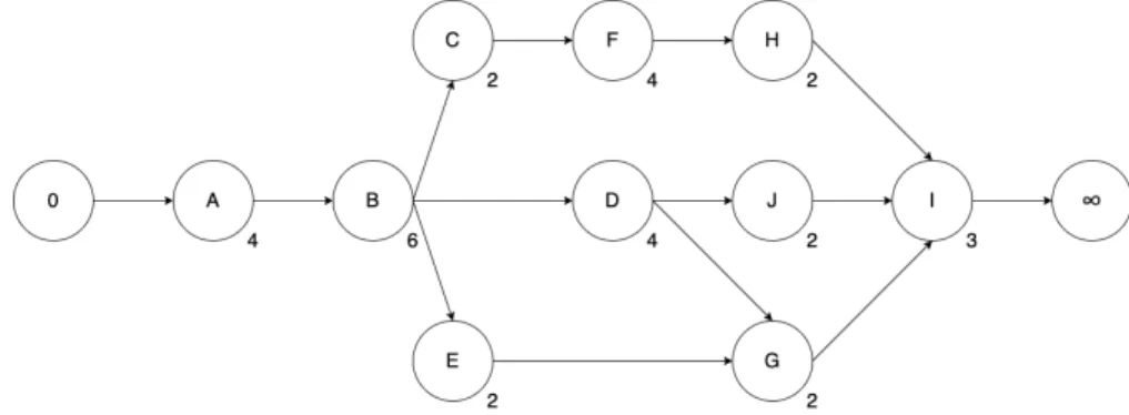
An example of a network diagram in which this situation appears is illustrated on Figure 6.7. Figure 6.7 is an adjustment of Figure 6.2. There is an extra activity J added. AJ has a duration of 1 and a resource need of 2.

The predecessor of AJ is AD and its successor is AI. This new diagram results in the same undirected edge as

Figure 6.3, namely D − F . It generates the same critical path as Figure 6.4 when giving the direction D → F to the undirected edge. This critical path is 0 → A → B → C → F → H → I → ∞. The differences start when scheduling this project. Since the critical path is the same as the critical path in Figure 6.4, the first scheduled activities will also be those that are illustrated in Figure 6.5. However, when scheduling the residual activities, there is an extra activity AJ. This results in 3 activities (AH, AG and AJ) that have t = 4 as start time

(STi). But since their combined resource need (RH1+ RG1+ RJ 1= 6) does not exceed the resource availability

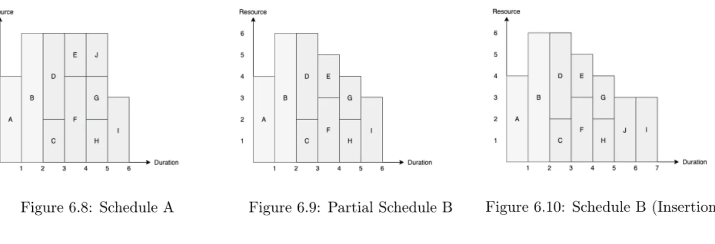
(RA1= 6), is this combination feasible. The complete schedule is visualised on Figure 6.8.

(40)

However, if 3 activities are combined it may be that the combination of these resource needs exceeds the available amount of resources. This case will be called situation B and does result in a problem. This happens for example, if AJfrom the network diagram on Figure 6.7 would need 3 units of R1instead of 2 units (RJ 1= 3).

When combining AJ, AGand AHon t = 4, the resource need exceeds the resource availability (RJ 1+RG1+RH1=

7 > 6 = RA1). To explain this problem AF from the network diagram in Figure 6.7 will also be altered so that

the resource need of this activity equals 3 (RF 1 = 3). The problem that now emerges, is illustrated on a

partial schedule in Figure 6.2.2.1. The scheduling of this example is done following the priority list (D, E, G, J ). The start time of activities AD, AE, and AG can be scheduled perfectly following the, until now, used method.

However, when scheduling the start time of AJ a problem emerges. On the schedule of Figure 6.8 the start time

of AJ is scheduled on t = 4. However, AJ requires 3 units of R1 and at t = 4 there are only 2 resources of R1

left. The first start time that has enough resources left for AJ is t = 5. Having said that, the start time of AI is

already scheduled on t = 5 and AJ has to be finished before AI can start, i.e. AI and AJ cannot have the same

start time. This creates a problem that the formerly method does not consider.

6.2.2.1 Simplification 2 - Insertion

The acquired solution for Problem 2 is a procedure called insertion. The insertion procedure will insert the problematic activity (in this case AJ) in the schedule. The right placement of the activity will be based on the

predecessors and the successors of the activity and the priority list. Successors will be pushed further down the schedule so that the start time of the problematic activity can be scheduled.

Example 6. For this example this results in assigning the start time t = 5 to AJ(STJ= 5) and pushing the

start time of AI to t = 6 (STI = 6). This location is based on the fact that AJ needs to be processed after AD

which is finished at t = 3 and that the start times of activities AE and AG are scheduled at t = 4 with a higher

priority value, i.e. AJ needs to be processed after t = 5. The completed schedule with the insertion procedure

is shown in Figure 6.10.

Figure 6.8: Schedule A Figure 6.9: Partial Schedule B Figure 6.10: Schedule B (Insertion)

This means that the formerly word for the duration of the critical path "makespan" is not equal the actual makespan with this method, i.e. the longest time in which the project can be executed. From now on makespan will no longer be used for the duration of the critical path. The duration of the critical path is the duration of the scheduled critical activities, before scheduling all residual activities that do not lie on the critical path. For

(41)

6.2.3 Problem 3 - Duration of the critical path vs. shortest makespan

The insertion method increases the duration of the project so that the duration of the critical path and the actual makespan may not have the same value as explained in Section 6.2.2.1. This leads to the fact that a solution with the shortest duration of the critical path might not have the shortest makespan. Example 7 will illustrate this problem.

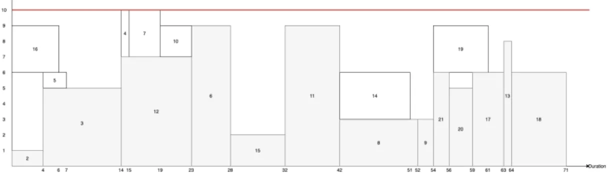
Example 7. Figures 6.11 and 6.12 show two different potential schedules of the same project. Both solutions have different directions for their edges. The critical path of solution A on Figure 6.11 is 1 → 2 → 3 → 12 → 6 → 15 → 11 → 8 → 9 → 21 → 20 → 17 → 13 → 18 → 22 and the duration of this critical path is 69 time units. The critical path of solution B on Figure 6.12 is 1 → 2 → 3 → 7 → 11 → 5 → 8 → 9 → 19 → 13 → 17 → 18 → 22 and the duration of this critical path is 61 time units. However, when scheduling the remaining activities, the makespan of solution A becomes 71 time units, while the makespan of solution B is 72 time units. The solution with the shortest duration of the critical path leads to the longest makespan. The critical activities are colored in grey and the non-critical activities are colored in white. Figure 6.12 shows how the insertion of activities 14 and 21 pushes the critical activities 13, 17, and 18 back. The makespan of solution B is bigger than the makespan of solution A because of this insertion.

Figure 6.11: Schedule Solution A.

(42)

6.2.3.1 Simplification 3 - Makespan

The goodness of a solution needs to be identified by the value of the makespan and not the duration of the critical path. The optimal direction of the edges can only be determined after all activities have been scheduled, and not after scheduling the critical activities. A full analysis of the relationship between the duration of the critical path and the makespan is done in Section 11.1.

6.2.4 Problem 4 - Critical arcs

The DG method for the JSSP focused on changing the direction of the critical arcs to find the optimal digraph. However, as stated above, the shortest duration of the critical path does not necessarily lead to the shortest makespan. Focusing on the direction of the critical arcs can thus leave out the optimal digraph.

Furthermore, the DG method for the RCPSP will generate more edges than for the JSSP due to the higher number of resource types and resource availabilities. It might thus be preferred to find an approximation of the solution instead of the exact solution as explained in Section 4.2.

6.2.4.1 Simplification 4 - Randomization

Because of the two, previously stated, reasons, the solution is found through randomization instead of optimiza-tion. The direction of the edges is generated randomly to create a potential schedule. Afterward, the makespan of that schedule is calculated. This is repeated a certain number of times and the minimum found makespan is then determined out of the generated options. The schedule that belongs to the minimum found makespan becomes the final solution.

(43)

7 |

The Basic algorithm

7.1 Input file

To be able to run the program on a specific network diagram, the network diagram has to be imported into the program. This is done with text files that have a predetermined structure. The composition of the information in the text file is shown below in Table 7.1. I represents the number of activities in a project. However, the number that is used by the program is I0. I0 is the number of nodes in a project and equals I + 2 as it includes all activities, including the start node and the end node. The index for the nodes will then also be i0 instead of i for activities, so the representation of node i0 becomes Ni0. Next the number of resource types (K) and the

maximum number of available units of resource type k per time unit t (RAk) are imported into the program.

After this, information about each node is imported into the program. Per node this includes; duration of node i0 (d0_i0), the number of units node i0 needs of resource type k per time unit t (R0_i0_k), the amount of successors

of node i0 (Yi0), and an enumeration of those successors where each successor has an index y_i0 (SS_y i0). d

0 1 and

R_1k0 ∀k should normally be equal to 0. This is because node 1 is the start node and has no duration or resource need. Just like node 1 should for node I0, d0_I0 and R_I00_k∀k also be equal to 0. As node I0 is the end node and

this results in no duration or resource need. YI0 should be equal to 0 as the end node has no successors.

I0 K RA1 ... RAK d0₁ R₁₁0 ... R_1K0 Y1 SS11 ... SSY1 .. . ... ... ... ... ... ... ... d0_I0 R0_I0₁ ... R0_I0_K YI0 SS₁ I0 ... SSYI0

Table 7.1: Structure input file.

7.2 Algorithm

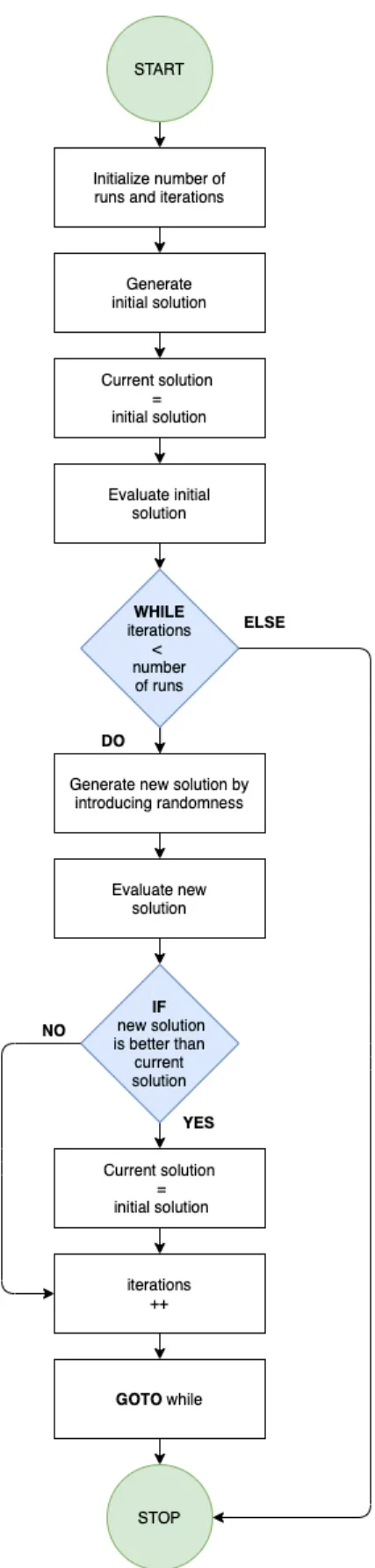
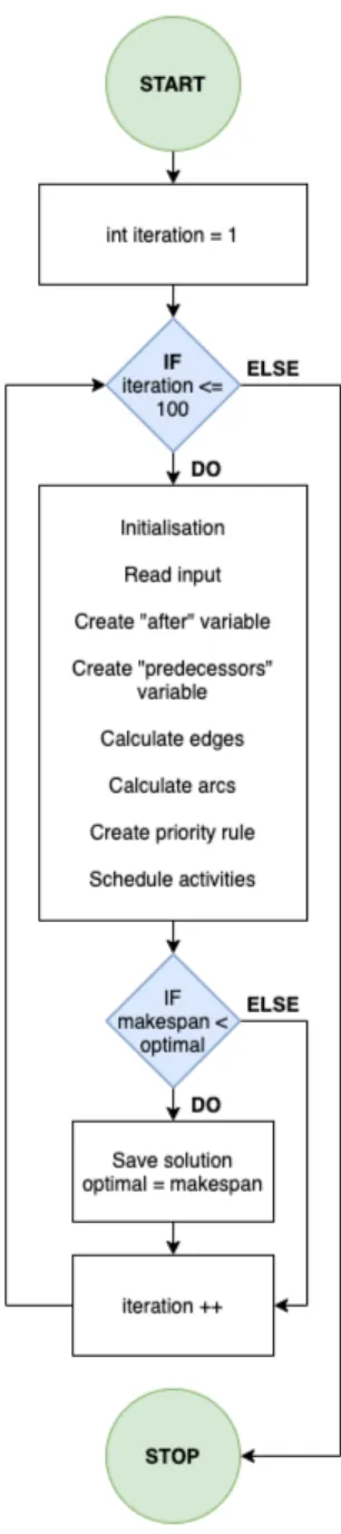
First, a flowchart is shown of the big building blocks of the algorithm in Figure 7.1. Afterward, a more detailed view and discussion of each building block is given. The algorithm includes an iteration of 100. This means that the algorithm will generate a 100 schedules. Every time a new schedule is generated, the makespan of the new schedule is compared with the current optimal makespan (i.e. the lowest makespan). If the makespan of the new schedule is lower, the solution of the schedule is saved. The solution of the schedule is printed to the output file and the newfound makespan becomes the current makespan. If the new schedule is suboptimal, the algorithm will generate a new schedule without saving the previous one.

(44)

Figure 7.1: Overview Algorithm

7.2.1 Initialization

In the initialization method all variables are initialized. This means that all parameters are assigned the value 0 and all vectors are cleared. Subsequently, all variables are given an initial value. This is an important step if there are repetitions in the algorithm. If there are iterations in the algorithm, this step makes sure that the iteration starts with empty values and does not calculate using values of the previous iteration.

(45)

7.2.2 Read Input

Next the input file needs to be imported into the program. The input file is the file discussed in section 7.1. The information about the project that needs to be scheduled is imported through this input file. Values are assigned to the variables that symbolize the number of nodes (I0), the amount of resources (K), the resource availabilities per resource (RAk), the duration of each node (d0i0), the resource need of each node (R0_i0_k), the

number of successors of each node (Yi0) and the successors in question (SS_y i0).

7.2.3 Create "after" Variable

An important variable that needs to be created before calculating the edges and arcs is the "after" variable. This variable makes sure that there are no unnecessary edges drawn. First, an example of such an unnecessary edge is given. In Figure 7.2, a network diagram is visualized in which the project has only one resource (K = 1) with a resource availability of 5 (RA1 = 5). When looking at the resource needs of the activities we see that

no activities can be executed in parallel. However, drawing an edge between activities A1 and A4 would be

unnecessary as there is already a precedence constraint between them. Another example are activities A1 and

A3 because A3 cannot occur until A1 is executed, drawing an edge would thus again be unnecessary.

0 1 1 1 1 1 0 0 1 1 1 1 0 0 0 1 0 1 0 0 0 0 0 1 0 0 0 1 0 1 0 0 0 0 0 0

Table 7.2: Example "after" Variable. Figure 7.2: Example Network Diagram Unnecessary Edges

Variable "after" is a two-dimensional boolean array. It indicates if an activity can only occur after another activity. For example if af ter[2][4] = 1, this means that node 4 (i.e. activity 3) cannot occur before node 2 (i.e. activity 1). So for Figure 7.2, an example of the variable "after" is illustrated in Table 7.2. Each row and each column represent a node (including the begin and end node). A 1 means that the column node cannot occur before the row node has been processed. So row 5, for example, indicates that node 5 (i.e. activity 4) has to be processed before node 4 (i.e. activity 3) and node 6 (i.e. end node).

7.2.4 Create "predecessors" Variable

When importing the input file into the program, a variable "successors" is created that contains all successors of each node. In this way the variable can give you all the successors of a node. In this step, a reverse variable is created. A "predecessors" variable is created that contains all predecessors of each node. So all predecessors of each node can additionally be requested through this variable. The number of predecessors of each node is symbolized with Xi0. And each predecessor is symbolized with P D_x

i0, where xi0 is the predecessor index. So for

Disjunctive arcs and resource flows in project networks