Application of the IPCC uncertainty methods to EDGAR 4.1 global greenhouse gas inventories

(1)

Application of the IPCC uncertainty methods to EDGAR 4.1 global

greenhouse gas inventories

Jos G.J. Olivier1, John A. van Aardenne2*, Suvi Monni2, Ulrike M. Döring2, Jeroen A.H.W. Peters1 and Greet Janssens-Maenhout2

1_{Netherlands Environmental Assessment Agency (PBL)} P.O. Box 303, NL-3720 AH Bilthoven, The Netherlands

jos.olivier@pbl.nl

2_{Joint Research Centre, Institute for Environment and Sustainability (JRC-IES)} Climate Change Unit, TP290, 2749, I-21027, Ispra (Va), Italy

* Now at European Environment Agency (EEA), Kongens Nytorv 6, 1050 Copenhagen K, Denmark

Introduction

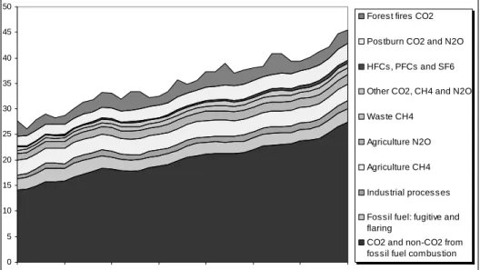
JRC and PBL have compiled a comprehensive EDGAR v4.1 global emissions dataset for the period 1970-2005 for the ‘six’ greenhouse gases included in the Kyoto Protocol (CO2, CH4, N2O, HFCs, PFCs and SF6), which was constructed using consistently the 2006 IPCC methodology and combining activity data (international statistics) from publicly available sources and for the first time - to the extent possible - emission factors as recommended by the IPCC 2006 guidelines for GHG emission inventories (Figure 1). This dataset, that covers all countries, provides independent estimates for all anthropogenic sources from 1970 onwards that are consistent over time and comparable between countries. Where appropriate emission abatement or recovery was taken into account, based on data reported by Annex I countries under the UN Climate Convention or based on other publicly available data sources. The resulting emissions of all gases identified in the Kyoto Protocol are reported using the 1996 IPCC source category classification for ease of recognition of the scope of each category and to allow for easy comparison with national greenhouse gas inventories reported by Annex I countries.

Thus we provide full and up-to-date inventories per country, also for developing countries that go beyond the mostly very aggregated UNFCCC reports of the developing countries. Of the 220 UN nations in 2005 only 43 industrialised countries (‘Annex I’) annually report their national GHG emissions in large detail from 1990 up to (presently) 2008, while most developing countries (‘non-Annex I’) for the UN Climate Convention (UNFCCC) and the Kyoto Protocol only report a summary table with emissions for one or more years (many only for 1994) (UNFCCC, 2005). More information on methods, data sources and differences with previous data is provided in the documentation available at the EDGAR 4 website: http://edgar.jrc.ec.europa.eu . Moreover, the time series back in time to 1970 provides for the UNFCCC trends a historic perspective. As part of our objective to contribute to more reliable inventories by providing a reference emissions database for emission scenarios, inventory comparisons and for atmospheric modellers, we strive to transparently and publicly document all data sources used (Olivier et al., 2010) and assumptions made where data was missing, in particular for assumptions made on the shares of technologies where relevant.

(2)

0 5 10 15 20 25 30 35 40 45 50 1970 1975 1980 1985 1990 1995 2000 2005

Forest fires CO2 Postburn CO2 and N2O HFCs, PFCs and SF6 Other CO2, CH4 and N2O Waste CH4

Agriculture N2O Agriculture CH4 Industrial processes Fossil fuel: fugitive and flaring

CO2 and non-CO2 from fossil fuel combustion

Figure 1. Trend in global greenhouse gas emissions 1970-2005 (unit: Pg CO2-eq.) (source: EDGAR 4.1)

Uncertainty in global and national greenhouse gas inventories

We present our estimate the global inventories of the main greenhouse gases and their trend by major source and region and the methods used to estimate the uncertainty in total regional and total global emissions and representative estimates at country level. Since the uncertainty estimates start with the data used at country level, we have aggregated sources and countries to regions where significant correlation of activity data or emission factor uncertainty exists between source categories or between countries, e.g. when using regional or global default emission factors (Olivier and Peters, 2002).

While using IPCC methodology and default emission factors whenever possible, this also allows us to use the default uncertainty estimates provided in the 2006 guidelines in most cases. Many Annex I countries may apply higher tier methods than was done for EDGAR 4.1 and may also apply country-specific emission factors rather than IPCC default values, that should in most cases result in lower uncertainties.

Uncertainty estimates are made for different reasons. In scientific inventories such as EDGAR and in official national GHG inventories. In scientific inventories, it is good scientific practice to assess and report on the uncertainty of the results as an expression of the overall quality of the resulting emissions as judged by the compilers. A preliminary estimate of uncertainties in global emissions of CH4 sources in EDGAR 3.2 based on IPCC default values appeared to be comparable with uncertainties estimated by global budget studies (Olivier, 2002). This is useful information for atmospheric modellers that require uncertainty estimates for all parameters in their model of which emissions are an important one, so the uncertainty in emissions is part of the overall uncertainty assessment of the model application. On the other hand, for official national greenhouse gas inventories uncertainty estimates are made just as a means for prioritising inventory improvement activities. Since the focus of these inventories lies in reporting emission inventories according to the guidelines, estimating uncertainties is often not given a high priority and IPCC default uncertainty values are applied. Knowing these different approaches to uncertainty estimates is pivotal information for using and interpreting these

(3)

different types of emissions inventories by the Earth System and Atmospheric Modelling communities.

Besides application in comparisons to other greenhouse gas inventories, emission uncertainty estimates are also important information for atmospheric modellers when estimating emissions (‘inferred emissions’) from measured atmospheric concentrations by so-called inverse modelling. Here a priori emissions are required with uncertainty estimates for each major sources and region to restrict the model to areas where emissions are believed to be most uncertain. Also uncertainty estimates for both emission datasets are required to assess their comparability. Inverse modelling of global or regional emissions has been done for several gases now, such as CH4 and HFC-134a (Villani et al., 2010). Recently more results on recent trends in F-gas emissions such as HFC-23 (Montzka et al., 2010), CF4, C2F6, F3F8 (Muhle et al., 2010) and SF6 (Levin et al., 2010; Rigby et al., 2010) have been published. The methods we applied in estimate uncertainties in total global emissions of our scientific inventory may also be used for combining official emission inventories reported by countries to the UNFCCC, e.g. for use in atmospheric models for verification purposes.

Comparison with official Annex I inventories

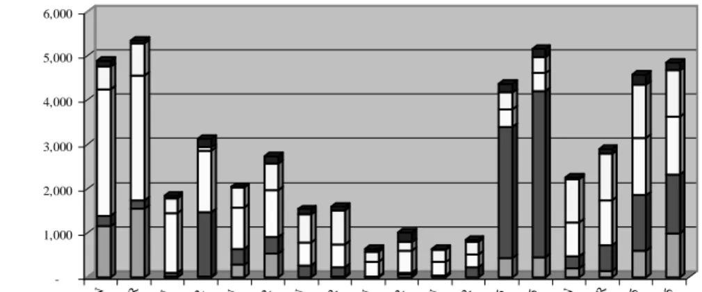
Apart from reporting the estimated uncertainty per source category, we also document the tier level of the methods used to compile the EDGAR 4.1 inventories. Therefore it is of interest to compare per category the difference between reported national emissions as well as reported uncertainty estimates for them and EDGAR estimates of emissions and their uncertainty. In Figure 2 we show comparisons for selected Annex I countries of emissions reported to the UNFCCC and EDGAR 4.1 estimates, for national total emissions (without uncertainty). In Figures 3 and 4 we compare emissions of major source sectors of CH4 and N2O for the same countries. Through this comparison we can assess whether or not the IPCC default methods and/or default emission factors show a significant bias for application by industrialised countries or that the uncertainty in the reported emissions is so large that no robust conclusion can be drawn. Except for some notable sources in particular countries most source estimates seem to agree reasonable, taking into account the uncertainties that often resemble the (default IPCC) uncertainty in the emission factors used. The notable exceptions have to be investigated further to determine the causes of the large differences: inconsistent activity data of national and international statistics, the use of very different country-specific emission factors due to country-country-specific circumstances, the use of high tier or country-specific methodology, a judgement error in selecting the emission factors or a calculation error.

If they would show a bias, this would warrant the use of asymmetrical uncertainty ranges when using lower tier IPCC methods or default factors. Moreover the comparison provides insight on the net gain of using higher tier methodology and allows identifying those regions or sectors where application of higher tier methodology would be most beneficial.

Since the uncertainty estimates start for the data used at country level, we have aggregated sources and countries to regions where significant correlation of activity data or emission factor uncertainty exists between source categories or between countries, e.g. when using regional or global default emission factors.

Areas where higher tier methods or country-specific emission factors instead of default IPCC factors will increase the inventory quality are:

(4)

Total CH4 emissions in 2005 (excl. LULUCF) -5,000 10,000 15,000 20,000 25,000 30,000

Australia France Germany Italy Japan Netherlands Russian Federation United Kingdom United States G g UNFCCC EDGAR4.1

Total N2O emissions in 2005 (excl. LULUCF)

-200 400 600 800 1,000 1,200

Australia France Germany Italy Japan NetherlandsRussian Federation United Kingdom United States G g UNFCCC EDGAR4.1

Figure 2. Comparison of national total CH4 (a) and N2O (b) emissions in 2005 between EDGAR 4.1 and UNFCCC for selected countries

(without LULUCF) (unit: Gg)

(a) CO2 emission factors for fuel combustion (1A). Natural gas, coal, petrol and

diesel in road transport are often used and in large amounts and therefore cover a large fraction of national GHG emissions. It is known that carbon contents of gas and coal can vary significantly, depending on where it is produced. Also Annex I reporting of petrol emission factors shows a considerable spread in values and a tendency to depart from the IPCC default values (see examples provided in Table 1). As we can see, determining a country-specific value for these fuels may improve the accuracy in this part of the inventory. In particular for natural gas and for diesel in road transport the IPCC defaults, although still within the estimated uncertainties, seem to be somewhat biased to the low side (by 4 and 2.5%). For coal this conclusion cannot be drawn from the table since the values reported by Annex I countries refer to total “solid fuel”, which may include not only coal, but also coal-derived gases such as coke oven gas and blast furnace gas as well as brown coal.

(5)

(b) CH4 emission factors for animals (4A) and rice production (4C) may be

improved compared to (region-specific) default values by using higher tier methods to determine these values. This is particularly relevant if the productivity (e.g. meat or milk production per animal) changes significantly over time or when the national circumstances result in different values of parameters that have been used to calculate regional default IPCC emission factor values in the 2006 IPCC guidelines1.

(c) CH4 from landfills and wastewater (6A and 6B). More up-to-date country-specific

information or estimates, such as of the amounts of MSW generated and the fraction landfilled, the waste composition and the Degradable Organic Carbon fraction, and their change over time, will improve the accuracy of the emission estimates.

(d) CO2 from large-scale biomass burning and deforestation and sinks from biomass

growth (5) The uncertainty of this category could be reduced by using more

detailed information. However due to the limited accuracy of the key parameters for the emissions and sinks calculation due to the variability in biomass types, their spatial distribution and the inherently limited knowledge of the extent of logging, burning and other forest degradation, will in general prevent making a quite accurate estimate of emissions and sinks. However, in case this source category is one of the largest key categories, more capacity to perform a more detailed assessment of changes over time will improve the emissions/sink estimates, albeit still rather uncertain.

-1,000 2,000 3,000 4,000 5,000 6,000 Au stra li a-UN Au stra li a-ED GA R Fra nce -U N Fra nce -E DG AR Ger man y-U N Ger man y-E DG AR Ital y-U N Ital y-E DG AR Jap an-U N Jap an-E DG AR Net her lan d s-UN Net her lan d s-ED GA R Ru ssia -U N/5 Ru ssia -E DG AR /5 UK -U N UK -E DG AR Un ited Sta te s-UN /5 Un ited Sta te s-ED GA R/5 Gg Sectoral CH4 emissions in 2005 6B 6A 4A 1B2 1B1

Figure 3. Comparison of sectoral CH4 emissions in 2005 between EDGAR 4.1 and UNFCCC data for selected countries: 1B1 – coal mining, 1B2 oil and gas, 4A –

animals, 6A – landfills, 6B - wastewater (unit: Gg) (Russia and USA *0.2)

1_{Note that the uncertainty of indirect N}

2O emissions from agriculture cannot be reduced due to the largely inherent uncertainty of this source category

(6)

-50 100 150 200 250 300 Aus tral ia-U N Aus tral ia-E DG AR Fra nc e-UN Fra nc e-ED GA R Ger man y-U N Ger man y-E DG AR Ital y-U N Ital y-E DG AR Japa n-U N Jap an-E DG AR Net her lan ds-U N Net herl and s-E DG AR Ru ssia -U N/2 Ru ssia -ED GA R/2 UK -U N UK -ED GA R Uni ted Sta te s-UN /4 Un ited Sta te s-ED GA R/4

Sectoral N2O emissions in 2005

6B 4D3 4D2 4D1oth 4D11 4B 2B 1A3b

Figure 4. Comparison of sectoral N2O emissions in 2005 between EDGAR 4.1 and UNFCCC data for selected countries: 1A3b – road transport, 2B –chemical industry, 4B – animal waste (stables), 4D11 – synthetic fertilisers, 4D1-other – other direct soil emissions, 4D2 – pacture, range, 4D3 –

indirect N2O, 6B - wastewtaer (unit: Gg) (Russia *0.5 and USA *0.25)

Table 1. Variability in CO2 factors from fuel combustion reported by Annex I countries and comparison with IPCC default values in the 2006 guidelines. Unit: kg/GJ (LHV). Uncertainties expressed as 2 standard deviations (SD). (source: UNFCCC, 2009)

Fuel type Sector IPCC default EF Unc. [%] Unc. (low) Unc. (high) Average EF reported Stand. dev. reported Unc. (low) Unc. (high) Diffe-rerence Diff- erence

coal residential sector 98.3 3.3 94.6 101.0 96.6 6.6% 83.9 109.3 -1.7 -1.7%

coal power generation

a) b) 94.6 5.4 89.5 99.7 99.0 8.1% 82.9 115.1 4.4 4.7% coal industry a) c) 94.6 7.2 87.3 101.0 99.5 22.9% 53.9 145.1 4.9 5.2% natural

gas all sectors 56.1 3.6 54.3 58.3 58.4 19.0% 36.2 80.6 2.3 4.1% petrol road transport 69.3 4.0 67.5 73.0 71.0 2.6% 67.3 74.7 1.7 2.5% diesel road transport 74.1 1.5 72.6 74.8 73.5 0.8% 72.3 74.7 -0.6 -0.8%

a) Less reliable for hard coal, since coal-derived gases such as coke oven gas and blast furnace gas as well as brown coal can be included here (Annex I countries refer to “solid fuel”). This is much less so for the residential sector.

b) For IPCC default value for other bituminous coal was used. c) For IPCC default value for coking coal was used.

Table 1 also provides another way to look at the uncertainty in using IPCC default emission factors, e.g. for CO2 from fuel combustion, is by assessing the spread in the values of specific emission factors and comparing the average of the country-specific values with the IPCC default value. This could only be done for a number of sectors and fuels for which the UNFCCC data refer to rather homogeneous fuel types.

(7)

Changes from 1996 to 2006 IPCC guidelines for GHG inventories

Please note that the emission factors used in EDGAR 4.1 are based on the 2006 IPCC guidelines, which may differ from the Revised 1996 IPCC guidelines. For many sources the changes are small, but for some, they can be significant. For CO2 emissions differences are due to the following reasons:

• national energy statistics used may differ slightly due to updates included in more recent releases, which may not be included in the data submitted to the IEA. For EDGAR 4.1 the release of 2007 was used (IEA/OECD, 2007);

• for the UNFCCC, if countries do not have country-specific emission factors, they will use the default CO2 emission factors from the Revised 1996 IPCC Guidelines, which differ slightly due to different default oxidation factors (coal updated value +2%, oil products +1%, natural gas +0.5%) and due to updated defaults for carbon content for some fuels of which the quality may vary considerably (mainly refinery gas, updated value -7%, coke oven gas -7%, blast furnace gas +7%, coke -1%);

• for CO2 from non-energy use or use of fuels as chemical feedstock countries may apply either higher tier methods using more country-specific information or calculate CO2 emissions from carbon released in fossil fuel use labelled in the sectoral energy balance as ‘non-energy use’ or ‘chemical feedstock’ using default fractions stored provided in the CO2 Reference Approach chapter. For EDGAR 4.1, default emission factors and methods from the 2006 IPCC Guidelines were applied, which may give rise to considerable differences compared to the 1996 guidelines.

For indirect N2O emissions from atmospheric deposition of NH3 and NOx emissions from agriculture as reported in EDGAR 4.1 are substantially lower than those presently reported by most Annex I countries due to two markedly lower emission factors compared to the values recommended in the 1996 IPCC Guidelines and the IPCC Good

Practice Guidance (IPCC, 1997, 2000):

• the default IPCC emission factor (“EF1”) for direct soil emissions of N2O from the use of synthetic fertilisers, manure used as fertiliser and from crop residues left in the field has been reduced by 20%;

• the default emission factor (“EF5”) for indirect N2O emissions from nitrogen leaching and run-off been reduced by 70%.

Thus our EDGAR 4.1 emissions can in some cases also be an indicator of how much emissions may change if countries use IPCC default emission factors and change them to the defaults in the 2006 IPCC guidelines.

Conclusions

EDGAR inventories are of interest for both Annex I and non-Annex I countries. For the first group they provide a measure to see the impact of using higher tier methodologies and more country-specific emission factors and technology information versus using IPCC standard methodology readily applicable by using widely available statistics as activity data and default emission factors. In other words, how the uncertainty in their national emissions estimate has improved compared to the less detailed default estimate. For the latter group of developing countries they provide an estimate of recent trend and level of national greenhouse gas emissions and assist in identifying the largest sources.

Using uncertainty estimates based on IPCC default uncertainty values seems at first sight a rather crude method. However, since the uncertainty in the various sources differs so widely, the results are likely to provide a fair estimate of the uncertainty in total

(8)

emissions per gas at national, regional and global level. The difference of EDGAR and official greenhouse gas emissions of Annex I countries also indicates the applicability of the tier 1 IPCC methodology and default emission factors to developing countries (within the uncertainty estimates).

References

IEA/OECD (2007, 2009). Energy Balances of OECD and Non-OECD Countries. On-line data service. Internet: http://data.iea.org

IPCC (1997). Revised 1996 IPCC Guidelines for National Greenhouse Gas Inventories. IPCC/OECD/ IEA, Paris.

IPCC (2000). Good Practice Guidance and Uncertainty Management in National Greenhouse Gas Inventories, IPCC-TSU NGGIP, Japan.

IPCC (2006). 2006 IPCC Guidelines for National Greenhouse Gas Inventories. Eggleston, S., Buendia, L., Miwa, K., Ngara, T., Tanabe, K. (eds.). IPCC-TSU NGGIP, IGES, Japan. Internet: http://www.ipcc-nggip.iges.or.jp/public/2006gl/index.html

Levin, I. et al. (2010). The global SF6 source inferred from long-term high precision atmospheric measurements and its comparison with emission inventories. Atmos. Chem. Phys., 10, 2655–2662, 2010.

Monzka, S.A. et al. (2010. Recent increases in global HFC-23 emissions. Geophys. Res. Lett., 37, L02808, doi:10.1029/2009GL041195.

Muhle, J. et al. (2010) Perfluorocarbons in the global atmosphere: tetrafluoromethane, hexafluoroethane, and octafluoropropane. Atmos. Chem. Phys., 10, 5145–5164, 2010. Olivier (2002) On the Quality of Global Emission Inventories. Approaches, Methodologies,

Input Data and Uncertainties. Thesis Utrecht University. Utrecht, Utrecht University. ISBN 90-393-3103-0. Internet: http://www.library.uu.nl/digiarchief/dip/diss/2002-1025-131210/inhoud.htm

Olivier, J.G.J. and J.A.H.W. Peters (2002) Uncertainties in global, regional and national emission inventories. In: Van Ham, J., A.P.M. Baede, R. Guicherit and J.F.G.M. Williams-Jacobse (eds.):‘Non-CO2 greenhouse gases: scientific understanding, control options and policy aspects. Proceedings of the Third International Symposium, Maastricht, Netherlands, 21-23 January 2002’, pp. 525-540. Millpress Science Publishers, Rotterdam. ISBN 90-77017-70-4.

Olivier, J.G.J., G. Janssens-Maenhout and J.A. van Aardenne (2010). Part III: Greenhouse gas emissions: 1. Shares and trends in greenhouse gas emissions; 2. Sources and Methods; Total greenhouse gas emissions. In: "CO2 emissions from fuel combustion, 2010 Edition”, pp. III.1-III.49. International Energy Agency (IEA), Paris (also available on CD ROM).

Rigby, M. et al. (2010) History of atmospheric SF6 from 1973 to 2008. Atmospheric Chemistry and Physics Discussions, Volume 10, Issue 5, 2010, pp.13519-13555

UNFCCC (2005). Sixth compilation and synthesis of initial national communications from Par-ties not included in Annex I to the Convention. Note by the secretariat. FCCC/SBI/2005/18, 25 October 2005. Internet:

http://unfccc.int/resource/docs/2005/sbi/eng/18.pdf

UNFCCC (2009). Sources and availability of GHG data for non-Annex I Parties. Internet: http://unfccc.int/ghg_data/ghg_data_unfccc/data_sources/items/3816.php. Retrieved 31 July 2009

Villani, M.G. et al. (2010) Inverse modeling of European CH4 emissions: sensitivity to the observational network. Atmos. Chem. Phys., 10, 1249–1267, 2010.

(9)

LVIV POLYTECHNIC NATIONAL UNIVERSITY

INTERNATIONAL INSTITUTE FOR APPLIED

SYSTEMS ANALYSIS

SYSTEMS RESEARCH INSTITUTE Polish Academy of Sciences

3rd International Workshop on Uncertainty

in Greenhouse Gas Inventories

PROCEEDINGS

LVIV POLYTECHNIC NATIONAL UNIVERSITY

Lviv, Ukraine

(10)

ISBN 978-966-8460-81-4

3rd International Workshop on Uncertainty in Greenhouse Gas Inventories, September 22-24, 2010, Lviv, Ukraine

Printed in the form submitted by authors.

Approved by the Scientific Committee of the 3rd International Workshop on Uncertainty in Greenhouse Gas Inventories, September 22-24, 2010, Lviv, Ukraine.

Acknowledgement

Publication was partially financed by the State Department of Environment Protection in Lviv Region, Ukraine.

Printed by “Print on Denand” – FOP Soroka S.V.

(11)

About the Workshop

The assessment of greenhouse gases (GHGs) emitted to and removed from the atmosphere is high on both political and scientific agendas internationally. Under the United Nations Framework Convention on Climate Change (UNFCCC), parties to the Convention have published national GHG inventories, or national communications to the UNFCCC, since the early 1990s. Methods for proper accounting of human-induced GHG sources and sinks at national scales have been stipulated by institutions such as the Intergovernmental Panel on Climate Change (IPCC) and many countries have been producing national assessments for well over a decade. However, as increasing international concern and cooperation aim at policy-oriented solutions to the climate change problem, a number of issues have begun to arise regarding verification and compliance under both proposed and legislated schemes meant to reduce the human-induced global climate impact.

The issues of concern at the International Workshops on Uncertainty in Greenhouse

Gas Inventories − the 1st Workshop was held on September 24-25, 2004, in Warsaw,

Poland; and the 2nd Workshop on September 27-28, 2007, in Laxenburg, Austria − are rooted in the level of confidence with which national emission assessments can be performed, as well as the management of uncertainty and its role in developing informed policy. The Workshops cover state-of-the-art research and developments in accounting, verifying and trading GHG emissions and provide a multidisciplinary forum for international experts to address the methodological uncertainties underlying these activities. The topics of interest center around national GHG emission inventories, bottom-up versus top-down emission analyses, signal processing and detection, verification and compliance, and emission trading schemes.

The 3rd International Workshop on Uncertainty in Greenhouse Gas Inventories took place September 22-24, 2010 at the Lviv Polytechnic National University (LPNU) in Lviv, Ukraine. This Workshop was jointly organized by the Austrian-based International

Institute for Applied Systems Analysis, the Systems Research Institute of the Polish Academy of Sciences, and the Lviv Polytechnic National University in Ukraine. Main

topics:

− achieving reliable national GHG inventories;

− accounting emissions across spatial scales (project, national, regional/continental);

− bottom-up versus top-down emission analyses;

− detecting and analyzing emission changes;

− reconciling short-term commitments and long-term targets;

− verification and compliance;

− trading emissions;

− communicating, negotiating and effectively using uncertainty.

Special attention was given to translating scientists’ understanding of uncertainty into options of use for policy makers to consider uncertainty in frameworks of negotiating climate change.

(12)

Scientific Committee

Chairmen:

Rostyslav Bun (Lviv Polytechnic National University, Ukraine) Zbigniew Nahorski (Polish Academy of Sciences, Poland) Members:

Yuri Ermoliev (International Institute for Applied Systems Analysis, Austria) Evgueni Gordov (Siberian Center for Environmental Research & Training,

Russia)

Giacomo Grassi (Joint Research Centre, Institute for Environment and

Sustainability, Italy)

Mykola Gusti (Lviv Polytechnic National University, Ukraine)

Khrystyna Hamal (Boychuk) (Lviv Polytechnic National University, Ukraine) -

Secretary

Javier Hanna (Reporting, Data and Analysis Programme, UNFCCC Secretariat) Olgierd Hryniewicz (Polish Academy of Sciences, Poland)

Matthias Jonas (International Institute for Applied Systems Analysis, Austria) Gregg Marland (Environmental Sciences Division, Oak Ridge National

Laboratory, USA)

Sten Nilsson (International Institute for Applied Systems Analysis, Austria) Krzysztof Olendrzyński (National Emission Centre, Poland)

Jaishankar Pandey (National Environmental Engineering Research Institute,

India)

Jean-Daniel Paris (Laboratoire des Sciences du Climat et de l'Environnement,

France)

Ariel Macaspac Penetrante (International Institute for Applied Systems

Analysis, Austria)

Stefan Pickl (Universität der Bundeswehr München, Germany)

Anatoly Shvidenko (International Institute for Applied Systems Analysis,

Austria)

Jochen Theloke (IER University of Stuttgart, Germany)

Isabel van den Wyngaert (Centre of Ecosystems, Alterra, The Netherlands) William I. Zartman (John Hopkins University, USA)

(13)

Application of the IPCC uncertainty methods to EDGAR 4.1 global greenhouse gas inventories