Flexible matrix multiplication kernels on GPUs

(1)

Flexible matrix multiplication kernels on GPUs

Academic year 2019-2020

Master of Science in Computer Science Engineering

Master's dissertation submitted in order to obtain the academic degree of Counsellor: Dr. Tim Besard

Supervisor: Prof. dr. ir. Bjorn De Sutter Student number: 01506418

(2)

(3)

Flexible matrix multiplication kernels on GPUs

Academic year 2019-2020

Master of Science in Computer Science Engineering

Master's dissertation submitted in order to obtain the academic degree of Counsellor: Dr. Tim Besard

Supervisor: Prof. dr. ir. Bjorn De Sutter Student number: 01506418

(4)

Permission of use on loan

The author gives permission to make this master dissertation available for consultation and to copy parts of this master dissertation for personal use. In all cases of other use, the copyright terms have to be respected, in particular with regard to the obligation to state explicitly the source when quoting results from this master dissertation.

(5)

Preface

Before you lies my master thesis “Flexible matrix multiplication kernels on GPUs”, the culmination of my studies Computer Science Engineering at Ghent University. This thesis is the result of my 9 month long journey through the LLVM compiler framework, GPU programming, the Julia programming language, and Julia’s GPU ecosystem. I have always been interested in compilers, and this thesis was an excellent opportunity to take this interest further. In particular, I enjoyed gaining experience with the widely used LLVM compiler framework. Additionally, I got the chance to explore GPGPU computing, a world which was new to me, using NVIDIA’s CUDA platform.

First and foremost, I would like to thank my supervisors Prof. Bjorn De Sutter and Dr. Tim Besard for their advice and guidance. Secondly, I want to thank the Julia community, in particular Valentin Churavy and Jameson Nash, for reviewing and merging my pull requests. Next, I want to extend my sincere gratitude to my parents, for their willingness to proofread drafts of this thesis, and for their unwavering support during my studies. Finally, I would like to thank you, the reader, for taking the time to read my thesis. I hope you enjoy reading it as much as I enjoyed writing it.

Thomas Faingnaert 1st July 2020

(6)

Flexible matrix multiplication kernels on GPUs

Thomas Faingnaert

Student number: 01506418

Supervisor: Prof. dr. ir. Bjorn De Sutter

Counsellor: Dr. Tim Besard

Master’s dissertation submitted in order to obtain the academic degree of Master of Science in Computer Science Engineering

Faculty of Engineering and Architecture, Ghent University Academic Year 2019 – 2020

Abstract

GEMM (General Matrix Multiplication) kernels are at the core of many computations in the fields of HPC (High Performance Computing) and ML (Machine Learning). GEMM is so prevalent that NVIDIA’s latest GPUs (Graphics Processing Units) include Tensor Cores, a special type of processing cores that are designed to accelerate matrix multiplications. As the fields of HPC and ML evolve, we notice two trends. First, the low-level programming language C++ that is traditionally used for high-performance applications, is being replaced by higher level languages such as Python or Julia. Through the use of the Julia package CUDAnative, one can even program GPUs directly in Julia. The second trend is the increasing need for flexibility in GEMM kernels. State-of-the-art GEMM libraries typically contain a limited set of monolithic kernels, and thus lack flexibility.

In this thesis, we will design, implement, and evaluate a GEMM framework for Julia that allows users to create GEMM kernels that are tailored to their use case. Given that NVIDIA’s Tensor Cores are already extensively used to accelerate ML and HPC workloads, we will mainly target GEMM using Tensor Cores. Our framework consists of three different APIs (Application Programming Interfaces). The first API provides an interface to access Tensor Cores from within Julia. The second API facilitates writing algorithms that use tiling techniques to improve performance, such as GEMM kernels. The final API consists of a set of customisable components that can be combined to implement a GEMM kernel for a specific purpose.

(7)

Flexible matrix multiplication kernels on GPUs

Thomas Faingnaert

Supervisor: Prof. dr. ir. Bjorn De Sutter Counsellor: Dr. Tim Besard

Abstract—GEMM (General Matrix Multiplication) kernels are at the core of many computations in the fields of HPC (High Performance Computing) and ML (Machine Learning). GEMM is so prevalent that NVIDIA’s latest GPUs (Graphics Processing Units) include Tensor Cores, a special type of processing cores that are designed to accelerate matrix multiplications. As the fields of HPC and ML evolve, we notice two trends. First, the low-level programming language C++ that is traditionally used for high-performance applications, is being replaced by higher level languages such as Python or Julia. Through the use of the Julia package CUDANATIVE, one can even program GPUs directly in Julia. The second trend is the increasing need for flexibility in GEMM kernels. State-of-the-art GEMM libraries typically contain a limited set of monolithic kernels, and thus lack flexibility.

In this thesis, we will design, implement, and evaluate a GEMM framework for Julia that allows users to create GEMM kernels that are tailored to their use case. Given that NVIDIA’s Tensor Cores are already extensively used to accelerate ML and HPC workloads, we will mainly target GEMM using Tensor Cores. Our framework consists of three different APIs. The first API provides an interface to access Tensor Cores from within Julia. The second API facilitates writing algorithms that use tiling techniques to improve performance, such as GEMM kernels. The final API consists of a set of customisable components that can be combined to implement a GEMM kernel for a specific purpose.

Index Terms—GPU, Julia, Tensor Cores, Flexible GEMM I. INTRODUCTION

Scientific computing applications typically rely on GPUs in-stead of CPUs, as the computational capabilities of the former are significantly larger than those of the latter. Traditionally, GPUs are programmed using low-level languages such as C++. As the field of scientific computing evolves, these low-level languages are being replaced with alternative languages with a higher-level syntax, but that are still able to match the performance of C++. The Julia programming language is an important example of a language with a high-level syntax, but a performance comparable to that of C++ [5]. Using the package CUDANATIVE, it is possible to program NVIDIA GPUs directly in Julia [4].

Matrix multiplication, commonly called GEMM (General Matrix Multiplication), is at the core of many computations in scientific computing. GEMM is used for neural networks in the field of ML (Machine Learning), and in several HPC (High Performance Computing) applications. Matrix multiplication

GPU vendors provide highly optimised implementations of GEMM in libraries, such as NVIDIA’s CUBLAS. These libraries contain a set of GEMM kernels designed for a specific purpose, and hence lack flexibility. This lack of flexibility is problematic if the needs of the application are not addressed by one of the kernels contained in the library. For example, inference in neural networks can be computed using a matrix multiplication, followed by the elementwise application of the activation function of the artificial neuron. Deep learning libraries typically only support a limited set of the most commonly used activation functions. This means that ML researchers cannot easily experiment with new activation functions without writing a performant GEMM kernel from scratch.

Another example is tensor contraction, the generalisation of matrix multiplication to multiple dimensions. One ap-proach for performant tensor contractions, GETT (GEMM-like Tensor-Tensor contraction), builds on top of a performant GEMM kernel [16]. GETT reshuffles the input tensors, so that the tensor contraction is equivalent to a matrix multiplication. This reshuffling can be performed before launching a pre-built GEMM kernel, but this introduces unnecessary overhead. This overhead can be avoided if the reshuffling is fused in the GEMM kernel instead. Of course, this is only possible if the underlying GEMM kernel is flexible.

Over the course of this thesis, we will design and implement a framework to instantiate customisable GEMM kernels on NVIDIA GPUs. We will use the high-level Julia programming language, and its package CUDANATIVE. Given their use in various ML and HPC workloads, we will mainly focus on GEMMs using NVIDIA’s Tensor Cores.

We will start with an introduction to the necessary back-ground information in Section II. This section discusses GPU programming, the Julia programming language, CUDANAT-IVE, and Tensor Cores. Our framework consists of three different APIs that interact. We will discuss each of these in a separate section. Section III describes the design of an API that allows us to use Tensor Cores from Julia. Next, Section IV discusses an API that facilitates writing algorithms that use tiling techniques to improve performance, such as matrix multiplications. The final API consists of a set of cus-tomisable components that together implement a performant GEMM kernel, and will be the subject of Section V. We will

(8)

II. BACKGROUND

This section discusses the relevant aspects of GPU pro-gramming, the Julia programming language, the Julia package CUDANATIVE, and Tensor Cores.

A. GPU programming

The main difference between programming GPUs versus CPUs is that the underlying programming model is different. GPUs are massively parallel processors, meaning that a large number of threads execute the same function in parallel. In GPU parlance, this function is commonly referred to as a kernel.

GPU threads are organised in a thread hierarchy [12]. Since our main interest is in NVIDIA GPUs, we will limit our discussion to NVIDIA’s CUDA programming model. In CUDA, the thread hierarchy consists of:

• Threads: Threads are the smallest unit of execution in the hierarchy.

• Warps: Threads are grouped by the hardware into a set of 32 threads called a warp. Threads in the same warp execute in a SIMT (Single Instruction Multiple Thread) fashion. This means that these threads must execute the same instruction at the same time, possibly on different data.

• Blocks: Threads are grouped by the programmer into blocks. Threads in the same block can communicate efficiently, so that they can cooperate on a common task. • Grid: The set of all blocks on the GPU device is called

the grid.

Similarly to threads, GPU memory is also ordered hierarch-ically. We are mainly interested in three parts of this hierarchy, corresponding to the levels in the thread hierarchy:

• Registers: The register file is the fastest type of memory. Each thread typically has access to 255 registers. • Shared memory: Each block has its own set of shared

memory, that may be used by threads in the same block to communicate.

• Global memory: Global memory can be accessed by all threads on the device, regardless of which block they belong to. Global memory has the largest capacity of the memory hierarchy, but also has much higher latency and lower throughput.

B. The Julia programming language

Julia is an open source programming language featuring a high-level syntax. A central paradigm in the design of the language is the way it handles dispatch, the process by which the compiler determines which implementation of a function to use for a given function call. Julia uses a multiple dispatch scheme, which means that this choice depends on the types of all of a function’s arguments [6].

Like most high-level languages, Julia’s type system is

features of its compiler. The Julia compiler applies type inference to deduce the types of values used by the program. If the compiler can deduce the types of all of the arguments in a function call, then this function can be specialised for these types. This specialised function is then compiled just-in-time to an efficient implementation, devoid of any dynamic type checks.

Julia’s compiler is built on top of LLVM, a compiler infra-structure project commonly used in research and industry [9]. Julia’s compilation process consists of a couple steps. First, Julia code is converted to an IR (Intermediate Representation) that is used for type inference, called Julia IR. Next, Julia IR is lowered to LLVM IR, the representation that LLVM uses. From this point onwards, the LLVM framework takes control of the compilation process. LLVM contains a set of backends, one for each target architecture that LLVM supports. The backend corresponding to the current architecture will then convert this LLVM IR to native instructions.

C. Programming GPUs in Julia using CUDAnative

CUDANATIVE is a Julia package that allows executing kernels written in Julia on NVIDIA GPUs. It reuses part of the Julia compilation process that we explained in the previous section. In particular, the compilation pipeline is run until the point where Julia IR is lowered to LLVM IR. The generated LLVM IR is intercepted, and sent to the LLVM NVPTX backend instead of the backend corresponding to the host architecture. This NVPTX backend converts LLVM IR to PTX instructions, the virtual instruction set of NVIDIA GPUs. NVIDIA GPUs are not capable of executing this PTX directly. PTX is first compiled by the GPU driver to SASS, the generation-specific instruction set that the GPU understands. D. Tensor Cores

Each Tensor Core performs a matrix multiply-accumulate, i.e. an expression of the form D = A·B+C. Tensor Cores only support a limited set of possible data types for these matrices. One peculiarity of these Tensor Cores is that the multiply-accumulate is performed in mixed precision. For example, if the A and B matrices are stored as 16-bit floating point values, the C and D matrices are 32-bit floating point.

NVIDIA exposes Tensor Cores in C++ in an API that they call WMMA (Warp Matrix Multiply Accumulate). As the name suggests, WMMA instructions must be used by all threads in a warp, in a SIMT fashion. Each thread that cooperates in a warp-wide WMMA operation holds a part of each matrix in its registers. This part is referred to as a fragment in WMMA terminology.

In WMMA parlance, we say that A is an M × K matrix, Bis a K ×N matrix, and C and D are M ×N matrices. The tuple (M, N, K) is called the shape of the WMMA operation. Note that not all possible values of M, N, and K are allowed, as WMMA restricts the set of possible shapes.

(9)

2) Perform the matrix multiply-accumulate using a WMMA mma operation, resulting in a fragment of the Dmatrix.

3) Store the resultant D fragment to memory using a WMMA store operation.

In CUDA C++, each of these steps corresponds to an over-loaded C++ function. Calls to these functions are converted to the correct WMMA PTX instructions by the CUDA C++ compiler.

III. ABSTRACTIONS FOR PROGRAMMINGTENSORCORES INJULIA

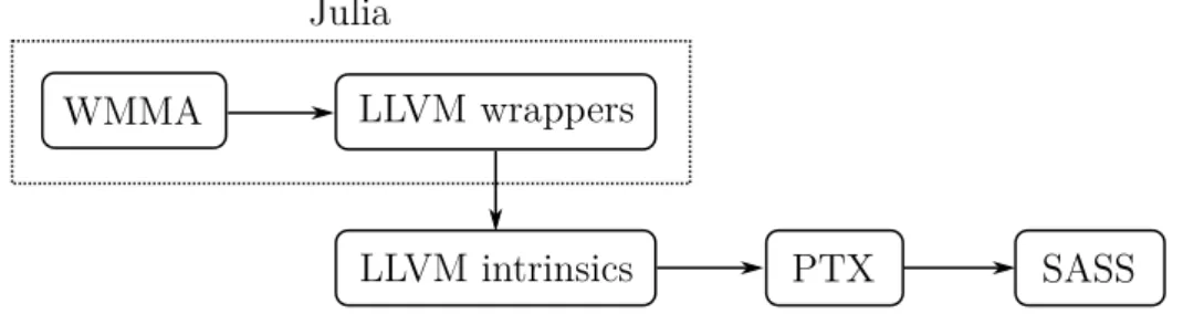
To support Tensor Cores in Julia, our WMMA API thus needs to make sure that CUDANATIVE generates the correct PTX instructions. We can reuse some existing functionality in the LLVM NVPTX backend for this purpose. In the context of compilers, an intrinsic or intrinsic function is a function that is handled in a special way by the compiler. Backends in the LLVM framework can define intrinsics that are specific to that backend. The NVPTX backend already includes intrinsics for WMMA, which are converted to the corresponding PTX instructions.

Our Julia API for Tensor Cores consists of two different layers. The first layer is a set of Julia functions that wrap the pre-existing intrinsics in the NVPTX backend. These wrapper functions are one-to-one, meaning that each intrinsic corresponds to one Julia function.

The Julia compiler already includes an llvmcall func-tion, that allows programmers to call LLVM intrinsics directly from Julia. The compiler first determines the Julia type of each of the arguments of llvmcall, converts these to the corresponding LLVM type, and inserts a call to the correct intrinsic. This mapping of Julia types to LLVM types is hardcoded in the Julia compiler. To support WMMA in Julia, we had to adapt this mapping, as the WMMA intrinsics use some LLVM types that did not have a corresponding Julia equivalent. We bundled the necessary changes to Julia’s code generation in one pull request, that has since been merged in the upstream Julia repository.

One possibility is to write these wrapper functions manually for each intrinsic, but that would be a very tedious process. Instead, we use Julia’s powerful metaprogramming capabil-ities to generate these wrappers automatically. We define a limited set of variables that contain the information necessary to generate these wrappers, such as the possible shapes of WMMA operations. We then simply iterate over the possible configurations, and dynamically generate the corresponding wrapper functions.

The second layer is a high-level interface, similar to CUDA C++’s version of WMMA. Each of the steps of WMMA corresponds to a different Julia function. For example, the A matrix is loaded with a call to load_a, and the resultant D matrix is stored to memory using store_d. Note that the

using a conf argument, which is a type that contains both the WMMA shape and accumulator element type. We then use Julia’s multiple dispatch mechanism to redirect calls to our high-level API to the correct intrinsic wrapper function.

Our WMMA API will serve as a building block to im-plement flexible GEMMs later on. One important operation that we must support for flexible GEMM is the application of elementwise transformations, such as linear scaling or ac-tivation functions in neural networks. To support elementwise operations, we integrate our WMMA API in Julia’s broad-casting framework. This way, we may apply an elementwise operation f to a WMMA fragment frag using Julia’s dot syntax: f.(frag). The resulting high-level WMMA API and intrinsic wrappers were bundled in one pull request, that has since been merged in CUDANATIVE.

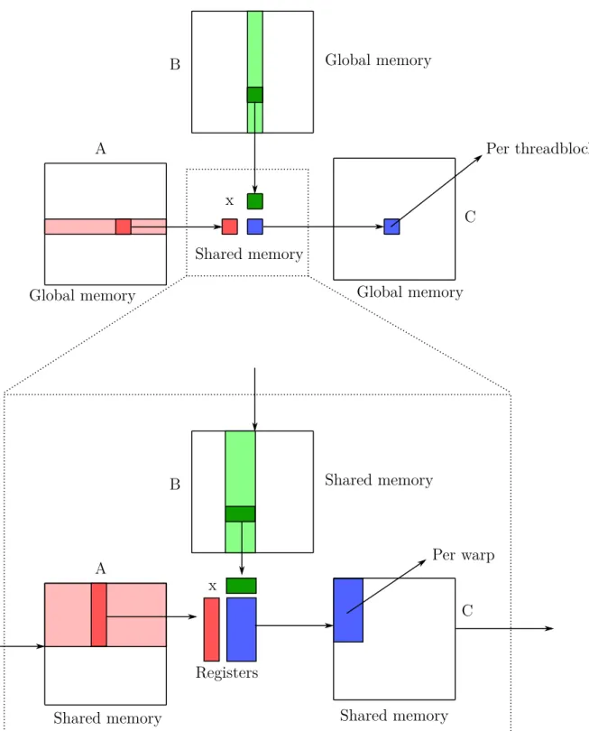
IV. ABSTRACTIONS FOR RECURSIVE BLOCKING Matrix multiplication is an application that is rich in data reuse. A matrix multiplication of square matrices of size N requires O(N3₎ _{floating point operations, but only O(N}2₎ storage. This results in each element being reused roughly O(N) times. This data reuse can be used to improve the performance of GEMM kernels. The general idea is to copy tiles of the input matrices from a slower type of memory to a faster type. This process is then repeated for every level in the memory hierarchy. The size of the tiles in each step is chosen such that they fit in the relevant part of the memory hierarchy. On the GPU, we first copy a tile from global memory to shared memory. We can then reuse the data in shared memory, which is faster than global memory loads. In a next step, we can load smaller tiles from shared memory to the register file. The massively parallel nature of GPUs allows us to improve performance of GEMM even further. Note that the computations of different tiles of the resultant matrix are independent, and can thus be performed completely in parallel. Recall that their is a one-to-one mapping between the levels of the thread and memory hierarchy. For example, shared memory is inherently linked to blocks, since only threads in the same block can communicate via shared memory. Each of the tiled copy operations is thus performed cooperatively, by all threads in the relevant part of the thread hierarchy. Consider the case of a GEMM D = A · B + C, where A is an M × K matrix, B is a K × N matrix, and C and D are M × N matrices. More concretely, this GEMM will consist of the following steps:

1) Copy a tile of C from global memory to shared memory, cooperatively by all threads in a block.

2) Copy a tile of C from shared memory to registers, cooperatively by all threads in a warp.

3) Iterate over the K dimension, according to the tiling size of a block.

(10)

c) Iterate over the K dimension, according to the tiling size of a warp.

i) Copy a tile of A from shared memory to registers, cooperatively by all threads in a warp. ii) Copy a tile of B from shared memory to registers, cooperatively by all threads in a warp. iii) Compute a tile of D, given the A, B, and C

tiles, cooperatively by all threads in a warp. 4) Copy a tile of D from registers to shared memory,

cooperatively by all threads in a warp.

5) Copy a tile of D from shared memory to global memory, cooperatively by all threads in a block.

Most GEMM implementations on NVIDIA GPUs use ex-plicit tiling to improve performance [11, 14, 10, 2, 8, 3]. Apart from GEMM, tiling is also used for batched GEMMs or tensor contractions [1, 3, 13, 7]. Given the multitude of different applications, a tiling API could prove very useful.

To that end, we have developed a tiling API in Julia that facilitates writing algorithms that use tiling techniques to improve performance. The most important operation in our tiling API is parallelisation. The parallelisation operation first divides a tile in subtiles of a given size. The resulting set of subtiles is then parallelised across all blocks on the device. Given a set of N subtiles and M blocks, each block will handle N

M subtiles. This parallelisation operation can be applied recursively. For example, the subtile of each block can be recursively parallelised across all the warps in the same block.

This parallelisation operation can be used to implement the general structure of a GPU GEMM that we described before. Our tiling API contains another operation that we call linearisation, that converts a tile to a linear offset in memory. Linearisation is used to calculate the memory address corresponding to each element in a tile. Our tiling API thus replaces the manual calculation of memory addresses, which is less maintainable, and more prone to errors.

The tiling API that we developed will be used as a building block to implement flexible matrix multiplication kernels in our GEMM API. Nevertheless, we have designed our tiling API to be as generally applicable as possible. For example, tiles in our API can have any number of dimensions, so that they can be used for tensor contractions as well.

V. ABSTRACTIONS FOR FLEXIBLE MATRIX MULTIPLICATION KERNELS

The final API in our flexible GEMM framework is the GEMM API itself. It uses the tiling API we described in the previous section to implement the general structure of a performant GEMM. Our API splits this GEMM kernel in a set of building blocks having a predetermined interface. Each of these building blocks corresponds to a way in which GEMM kernels need to be adapted, and can have different

block would include a column major, and a row major storage format.

Each of these building blocks corresponds to one or more calls to a set of functions with a predetermined name. For example, the building block that determines how A is stored can have two functions load and store that load and store a tile of A, respectively. The first argument to these functions is a type, such as ColumnMajor or RowMajor, that determines the memory layout of A. Using Julia’s multiple dispatch mechanism, we can customise the behaviour of these functions depending on this type, thereby adding flexibility to our GEMM kernel.

Note that the introduction of flexibility using this approach has no performance impact at runtime. Through type inference, the Julia compiler is able to infer the types passed to the load or store functions. The same applies to all different building blocks, so that it is known at compile time which implementations of each function will be called. These imple-mentations are then combined, and compiled just-in-time to a kernel tailored to a specific use case.

Of course, the most important question we should answer is which building blocks we need to cover a wide range of different use cases. To answer this question, we drew inspiration from two sources. First, we looked into NVIDIA’s open source CUTLASS library, which contains a set of components for performant GEMM or GEMM-like kernels. Second, we conducted a literature search to get an idea of the most common ways in which GEMM kernels need to be adapted. From these two sources, we propose 5 different building blocks: params, layouts, transforms, operators, and epilogues.

The params building block contains a set of fields that determine the tiling sizes that should be used for each step of the GEMM kernel. For example, the BLOCK_SHAPE field determines the size of the tiles loaded and stored by each block. The params building block also contains information regarding the launch configuration of the kernel, such as the number of warps per block.

The tiling sizes in the params component are specified in logical coordinates, i.e. with a meaning specified by the user. To load and store tiles, we need to convert this logical index to a physical offset in memory. This conversion is handled by the layout building block. Possible implementations of this building block are RowMajor and ColMajor. To provide maximal flexibility, users can specify the memory layout separately for each matrix, and for each level of the memory hierarchy. For example, the A matrix may be stored differ-ently in global and shared memory. This is especially useful for shared memory, as accessing shared memory efficiently typically requires more complicated memory layouts.

Transforms are arbitrary Julia functions that are automat-ically called after every load, and before every store. Their main use case is to apply elementwise transforms to the

(11)

networks.

Operators determine how the computation of the matrix product is performed in the inner loop. Possible implement-ations of this building block include a WMMA operator that performs the computation using Tensor Cores, or an imple-mentation that uses the traditional floating point hardware instead.

The final component in our GEMM API is the epilogue. As the name suggests, the epilogue building block is situated at the very last stage of GEMM. It offers more control than the layouts over how tiles of the resultant matrix are copied from shared memory to global memory. For example, a custom epilogue could apply a reduction operation over the tiles stored in shared memory across all blocks.

VI. EVALUATION

To evaluate the performance and flexibility of our frame-work, we will implement three different GEMM variants using our GEMM API. The first example is a normal mixed-precision GEMM that uses Tensor Cores via our WMMA API. Next, we introduce the necessary components to extend this GEMM to matrices of complex numbers. Our last example will change this complex GEMM so it also supports dual numbers. We will compare the performance of our GEMM kernels with the state-of-the-art GEMMs in NVIDIA’sCUBLAS and CUTLASS libraries. CUDANATIVE dispatches matrix multi-plications to cuBLAS, but only for datatypes that are com-patible with CUBLAS. For other datatypes, CUDANATIVE includes a generic kernel as a fallback. We will also compare our performance with CUDANATIVE’s generic implementa-tion.

A. Mixed-precision GEMM

To support a mixed-precision GEMM in our GEMM API, we will create an operator that builds on top of our WMMA API. This operator simply calls the correct WMMA function for each step in the GEMM’s inner loop.

Since Julia is column major, we also implemented a ColMajor layout component. This layout is suitable for global memory, but leads to inefficient memory accesses for shared memory. On NVIDIA GPUs, shared memory is split into memory banks. Different memory banks can be accessed in parallel, but memory accesses to addresses that map to the same bank are serialised. This serialisation process is often referred to as a bank conflict.

The most common way to reduce these bank conflicts for a column major layout, is to add padding to every column. This changes the mapping of matrix elements to banks, thereby reducing the number of bank conflicts. To introduce padding in our GEMM API, we added another layout PaddedLayout. The way this layout works is slightly different than ColMajor. It does not specify the mapping of logical indices to physical offsets directly, but is a wrapper for

The epilogue we use for our mixed-precision GEMM simply copies the corresponding tile from shared memory to global memory. Finally, we can implement a custom transform to apply elementwise operations such as scaling to the input matrices or the result of the matrix multiplication.

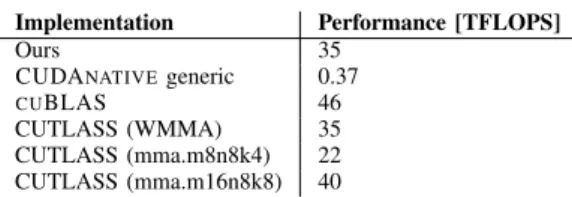
Table I compares the peak performance of our GEMM ker-nel with the generic implementation in CUDANATIVE, and the state-of-the-art implementations in cuBLAS and CUTLASS. CUDANATIVE’s generic kernel uses no tiling techniques, and is only able to achieve a peak performance of 0.37 TFLOPS. The CUTLASS (WMMA) implementation uses the same para-meters as our implementation: the tiling sizes are the same, and the matrix product in the inner loop is also computed using WMMA. We notice a perfect performance parity between this CUTLASS kernel and our implementation.

Both our implementation and CUTLASS (WMMA) achieve a performance of about 75% that ofCUBLAS. To understand this gap, we have also benchmarked two other kernels in the CUTLASS library. These kernels also use Tensor Cores, but do so using mma instructions instead of the WMMA API. These mma instructions are specific to the GPU generation, and allow more direct control over Tensor Cores compared to the portable WMMA abstraction layer. The performance results of Table I were obtained using an NVIDIA RTX 2080 Ti, which is a GPU of the Turing-generation. The mma.m16n8k8 instruction is optimised for Turing GPUs, and gets very close to CUBLAS’s performance. We also benchmarked a mixed-precision GEMM using the mma.m8n8k4 instruction, which is aimed at Volta GPUs, Turing’s predecessor. As we can see, the performance of this Volta-style mma is even worse than WMMA, indicating that these mma instructions are highly generation specific.

Table I

ACOMPARISON OF THE PEAK PERFORMANCE OF OUR MIXED-PRECISION

GEMMKERNELS WITH THE STATE-OF-THE-ART(HIGHER IS BETTER). Implementation Performance [TFLOPS]

Ours 35

CUDANATIVEgeneric 0.37 CUBLAS 46 CUTLASS (WMMA) 35 CUTLASS (mma.m8n8k4) 22 CUTLASS (mma.m16n8k8) 40 B. Mixed-precision complex GEMM

To implement a mixed-precision GEMM of complex num-bers, we can reuse most of the components of our previous example. There are only two main differences between a nor-mal mixed-precision GEMM, and a mixed-precision complex GEMM [2].

First, the WMMA multiply-accumulate operation in the inner loop is replaced by four WMMA operations: A.real * B.real, A.real * B.imag, A.imag * B.real, and A.imag * B.imag. In our GEMM API, this can be

(12)

imple-The second difference between normal GEMMs and com-plex GEMMs, is the memory layouts that are used. In global memory, complex matrices are stored in an interleaved layout, where the real and imaginary parts of the same element are stored contiguously in memory. To load the real and imaginary parts from shared memory into WMMA fragments, we need to use a split-complex layout. This layout stores the real and imaginary parts of the matrix separately. This is needed because WMMA implicitly assumes that elements in the same column of a column major matrix are stored at adjacent memory addresses. In our GEMM API, this can be done using two new layout components: InterleavedComplex and SplitComplex.

Table II shows the peak performance of our complex GEMM, CUDANATIVE’s generic implementation, and CUT-LASS. At the time of writing, CUTLASS only includes an mma variant of complex GEMM, so we cannot compare our implementation with CUTLASS’s WMMA. Still, we were able to achieve about 50% of the performance of CUTLASS’s mma kernel, without implementing any optimisations specific to complex GEMM. Once again, we see that our flexible kernel significantly outperforms the generic implementation in CUDANATIVE.

Note that the gap between our WMMA kernel and CUT-LASS’s mma is larger for complex GEMM than for nor-mal mixed-precision GEMM. This is likely because complex GEMMs have higher arithmetic intensity: the multiplication of two complex numbers requires four real multiplications. This means that the importance of the compute stage of GEMM increases, so that replacing WMMA with mma is more important for complex GEMM than for normal GEMM.

Table II

ACOMPARISON OF THE PEAK PERFORMANCE OF OUR COMPLEX MIXED-PRECISIONGEMMWITH THE STATE-OF-THE-ART(HIGHER IS

BETTER).

Implementation Performance [TFLOPS]

Ours 22

CUDANATIVEgeneric 1.2 CUTLASS (mma.m16n8k8) 42.7

C. Mixed-precision dual GEMM

In our final example, we study the case of the multiplication of matrices containing dual numbers. Dual numbers extend the set of real numbers with a new element ε, similar to the imaginary unit i in the case of complex numbers. Addition and multiplication of dual numbers is similar to the complex case, with the only difference that ε2 _{= 0, whereas i}2 ₌ _{−1. An} example application of dual numbers in scientific computing is automatic differentiation of functions [15].

Because of the similarity between complex numbers and dual numbers, most of the discussion of the previous example

the operator component. Instead of four WMMA multiplic-ations, we only need to perform three: A.real * B.real, A.real * B.dual, and A.dual * B.real. The use cases of complex and dual numbers are thus an excellent illustration of the reusability of the components in our GEMM API.

Performance-wise, we observe similar behaviour as the complex GEMM in the previous subsection. This is not surprising, as the only difference between complex and dual GEMMs is the operator used in the inner loop. Note that neitherCUBLAS nor CUTLASS include kernels that multiply matrices of dual numbers. Thus, multiplying dual matrices stored on the GPU in Julia will dispatch to CUDANATIVE’s generic implementation, which is many orders of magnitude slower than peak device performance. This means that using our GEMM API already results in a significant speedup for dual matrices, even though we can still improve the perform-ance of our complex and dual GEMMs.

VII. CONCLUSION

We designed, implemented, and evaluated a framework to instantiate flexible GEMM kernels on GPUs using the Julia programming language. We build on top of CUDANATIVE, a Julia package that compiles Julia code to the GPU’s PTX instruction set using the LLVM NVPTX backend. Our frame-work consists of three separate APIs.

The first API allows Julia kernels to program Tensor Cores, a type of processing core in the latest NVIDIA GPUs that ac-celerate matrix computations. This API consists of two layers: a low-level layer that directly wraps the correct intrinsics in the LLVM NVPTX backend, and a high-level WMMA API that is similar to the way Tensor Cores are exposed in CUDA C++.

The second API is a tiling API, and aims to facilitate writing algorithms that make use of tiling techniques. These tiling techniques are used in GEMM kernels, batched GEMM kernels, and tensor contractions to improve performance.

Finally, our third API consists of a set of components that together implement a GEMM. These components can be customised by the user, thereby introducing the necessary flexibility in the GEMM kernel.

We have evaluated the performance and flexibility of our framework using three different examples: a normal mixed-precision GEMM, a complex GEMM, and a dual GEMM. Our kernels perform similarly to the state-of-the-art imple-mentations in the CUTLASS library, provided that the same parameters are used. We also indicated how we could bridge the remaining performance gap with CUBLAS by using the generation-specific mma instructions instead of the portable WMMA interface.

REFERENCES

[1] A. Abdelfattah, S. Tomov and J. Dongarra. ‘Fast Batched Matrix Multiplication for Small Sizes Using

(13)

[2] A. Abdelfattah, S. Tomov and J. Dongarra. ‘Towards Half-Precision Computation for Complex Matrices: A Case Study for Mixed Precision Solvers on GPUs’. In: 2019 IEEE/ACM 10th Workshop on Latest Advances in Scalable Algorithms for Large-Scale Systems (ScalA). 2019, pp. 17–24.

[3] Ahmad Abdelfattah et al. ‘Performance, Design, and Autotuning of Batched GEMM for GPUs’. In: High Performance Computing. Ed. by Julian M Kunkel, Pavan Balaji and Jack Dongarra. Cham: Springer In-ternational Publishing, 2016, pp. 21–38. ISBN: 978-3-319-41321-1.

[4] T. Besard, C. Foket and B. De Sutter. ‘Effective Ex-tensible Programming: Unleashing Julia on GPUs’. In: IEEE Transactions on Parallel and Distributed Systems 30.4 (2019), pp. 827–841.

[5] JuliaLang.org. Julia Micro-Benchmarks. 2020. URL: https://julialang.org/benchmarks.

[6] JuliaLang.org. The Julia Language Official Document-ation. 2020. URL: https://docs.julialang.org/en/v1. [7] Jinsung Kim et al. ‘A Code Generator for

High-Performance Tensor Contractions on GPUs’. In: Pro-ceedings of the 2019 IEEE/ACM International Sym-posium on Code Generation and Optimization. CGO 2019. Washington, DC, USA: IEEE Press, 2019, pp. 85–95. ISBN: 9781728114361.

[8] J. Lai and A. Seznec. ‘Performance upper bound ana-lysis and optimization of SGEMM on Fermi and Kepler GPUs’. In: Proceedings of the 2013 IEEE/ACM Inter-national Symposium on Code Generation and Optimiz-ation (CGO). 2013, pp. 1–10.

[9] LLVM contributors. The LLVM Compiler Infrastructure Project. 2020.URL: https://llvm.org.

[10] Rajib Nath, Stanimire Tomov and Jack Dongarra. ‘An Improved MAGMA GEMM For Fermi Graph-ics Processing Units’. In: International Journal of High Performance Computing Applications 24.4 (Nov. 2010), pp. 511–515. ISSN: 1094-3420. DOI: 10.1177/ 1094342010385729. URL: http://dx.doi.org/10.1177/ 1094342010385729.

[11] NVIDIA. cuBLAS: CUDA Toolkit Documentation. 2020. URL: https://docs.nvidia.com/cuda/cublas/index. html.

[12] NVIDIA. CUDA C++ Programming Guide. 2020.URL: https://docs.nvidia.com/cuda/cuda- c- programming-guide.

[13] NVIDIA. cuTENSOR: A High-Performance CUDA Lib-rary for Tensor Primitives. 2020. URL: https : / / docs . nvidia.com/cuda/cutensor/index.html.

[14] NVIDIA. CUTLASS: CUDA Templates for Linear Al-gebra Subroutines. 2020. URL: https : / / github . com / NVIDIA/cutlass.

[15] J. Revels, M. Lubin and T. Papamarkou.

‘Forward-[16] Paul Springer and Paolo Bientinesi. Design of a high-performance GEMM-like Tensor-Tensor Multiplication. 2016. arXiv: 1607.00145 [cs.MS].

(14)

List of Figures

2.1 An overview of each component in the CUDA thread hierarchy, along with the corresponding level in the memory and hardware hierarchy. . . 7 2.2 An overview of the compilation pipeline of the Julia compiler. . . 9 2.3 An overview of Julia’s compilation pipeline adapted by CUDAnative.jl. . 12 3.1 An illustration of the TTGT algorithm for tensor contractions. . . 22 4.1 An overview of Julia’s compilation pipeline adapted by CUDAnative.jl. . 31 4.2 A schematic overview of the WMMA API that we will develop for Julia

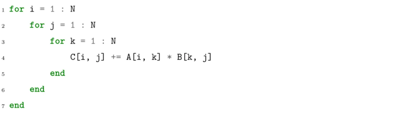
(top) and the pre-existing components it relies on (bottom). . . 32 5.1 An illustration of the triple loop nest approach to GEMM. . . 51 5.2 An illustration of the blocking approach applied to the GEMM problem

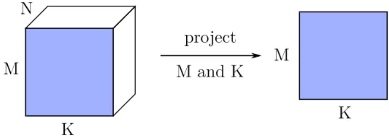
on GPUs. . . 53 5.3 An illustration of the projection of a three dimensional tile to two

dimen-sions M and K. . . 56 5.4 An illustration of the parallelisation of a tile over a set of 8 cooperating

warps. . . 58 5.5 An illustration of the translation of a tile. . . 59 5.6 An illustration of the conversion of a tile to a linear index. . . 59 5.7 A parallelisation operation over 2 warps handling a 4 × 2 set of subtiles in

parallel. . . 65 5.8 An illustration of copying a tile of the C matrix from global memory to

(17)

5.9 An illustration of the three dimensional iteration space in the inner loop of the matrix product. . . 75 5.10 An illustration of the computation of the matrix product in the innermost

loop. . . 76 5.11 An illustration of copying a tile of the D matrix from registers to shared

memory. . . 79 6.1 Copying a tile of A from global to shared memory using the params,

layouts, and transforms components in our GEMM API. . . 92 6.2 Storing a 4 × 4 matrix in shared memory in a non-padded layout. . . 104 6.3 Storing a 4 × 4 matrix in shared memory using padding. . . 104 6.4 A comparison of the performance of our mixed-precision GEMM with

state-of-the-art implementations on the NVIDIA V100 GPU. . . 105 6.5 A comparison of the performance of our mixed-precision GEMM with

state-of-the-art implementations on the NVIDIA RTX 2080 Ti GPU. . . 107 6.6 The difference between an interleaved and split memory layout to store

matrices of complex numbers. Memory addresses increase from left-to-right, and then from top-to-bottom, i.e. in a row-major fashion. . . 109 6.7 An illustration of the performance of our mixed-precision complex GEMM

on the NVIDIA V100 GPU. . . 110 6.8 An illustration of the performance of our mixed-precision complex GEMM

(18)

List of Abbreviations

API Application Programming Interface.

AST Abstract Syntax Tree.

ATLAS Automatically Tuned Linear Algebra Software.

BF16 Bfloat16.

BLAS Basic Linear Algebra Subprograms.

BLIS BLAS-like Library Instantiation Software.

CPU Central Processing Unit.

CTA Cooperative Thread Array.

CUDA Compute Unified Device Architecture.

CUTLASS CUDA Templates for Linear Algebra Subroutines.

DL Deep Learning.

(19)

FP16 Half Precision Floating Point.

FP32 Single Precision Floating Point.

FP64 Double Precision Floating Point.

FPU Floating Point Unit.

GEMM General Matrix Multiplication.

GETT GEMM-like Tensor-Tensor contraction.

GPGPU General-purpose computing on graphics processing units.

GPU Graphics Processing Unit.

GTC GPU Technology Conference.

HPC High Performance Computing.

IR Intermediate Representation.

ISA Instruction Set Architecture.

JIT Just-In-Time.

LoG Loop-over-GEMMs.

(20)

MAGMA Matrix Algebra on GPU and Multicore Architectures.

MKL Math Kernel Library.

ML Machine Learning.

OpenCL Open Computing Language.

OpenGL Open Graphics Library.

PTX Parallel Thread Execution.

SASS Streaming Assembler.

SIMT Single Instruction Multiple Thread.

SM Streaming Multiprocessor.

SSA Static Single Assignment.

TBLIS Tensor BLIS.

TF32 TensorFloat-32.

TTGT Transpose-Transpose-GEMM-Transpose.

(21)

1 Introduction

The days where GPUs (Graphics Processing Units) were only used as a coprocessor to perform graphics-related tasks have long since passed. Due to their massively parallel nature, GPUs can be used to significantly accelerate scientific computations as well. The use of GPUs for these purposes is commonly referred to as GPGPU (General-purpose computing on graphics processing units) programming. Several fields use GPUs to increase performance, including ML (Machine Learning) and HPC (High Performance Computing) [1, 61, 22, 18, 43].

GPGPU programming is typically performed in low-level languages such as C++, whereas researchers would prefer to use a high-level language such as Python or Matlab. Tradi-tionally, the choice between high-level or low-level languages comes down to a trade-off between performance and programmer productivity. Through the use of modern compiler techniques, it is possible to eliminate this trade-off and use a high-level language without sacrificing performance. Julia is one example of a programming language with a high-level syntax, but performance comparable to that of C++ [25]. Using the CUDAnative project, researchers are even able to program GPUs directly in Julia.

Matrix multiplication, commonly called GEMM (General Matrix Multiplication), is at the core of many computations in ML and HPC, ranging from neural networks to earthquake simulation and weather prediction [1, 33, 22, 43]. The multiplication of matrices is so prevalent that NVIDIA has introduced Tensor Cores in their latest GPUs. Tensor Cores are hardware units specifically designed to compute matrix multiplications quickly. One peculiarity of these Tensor Cores is that the matrix multiplication is performed in mixed precision, meaning that both 16-bit and 32-bit floating point is used during

(22)

the computation. The use of mixed precision has resulted in significant speedups in the training of neural networks and in several HPC applications [50, 18].

Efficient implementations of GEMM are bundled in vendor-specific libraries, such as cuBLAS in the case of NVIDIA GPUs. These libraries contain a set of pre-optimised GPU functions, called kernels, that are built for a specific purpose, and hence lack flexibility. This is problematic if the variant of GEMM needed for a given algorithm is not supported. In those cases, programmers typically have to spend a significant amount of time and effort implementing a performant kernel from scratch.

The focus of this thesis is the design and implementation of a high-level framework to instantiate performant GEMM kernels on GPUs. To increase programmer productivity, we will use the high-level programming language Julia and the package CUDAnative instead of C++. Given the prevalence of mixed precision in both ML and HPC, the end goal is a GEMM targetting NVIDIA’s Tensor Cores that is both performant and flexible. We will work towards this goal in three main steps.

Tensor Cores can be programmed in C++ using NVIDIA’s WMMA API (Application Programming Interface), which CUDAnative did not originally support. The first goal is thus the design and implementation of an API to interact with Tensor Cores from within Julia.

Once we can program Tensor Cores directly in Julia, we can use them to implement a matrix multiplication kernel. A possible approach is to divide the output matrix in small tiles, and to calculate each of these tiles using Tensor Cores. As we shall see, this implementation does not use the computational capabilities of the GPU optimally, and is hence extremely inefficient. The next goal is thus to research the design principles behind performant matrix multiplication kernels on GPUs, and to apply these principles to implement a performant mixed-precision GEMM.

Finally, we need to make this performant GEMM kernel flexible. To achieve this, we first conduct a literature search to understand which types of flexibility are important, and how other frameworks approach this requirement. From this search, we will distil a

(23)

list of the main use cases for flexible matrix multiplication kernels, and propose a set of abstractions needed to cover them. As a final step, we will introduce this flexibility in the mixed-precision GEMM kernel that we developed.

We will start with an introduction to the necessary background information regarding GPU computing, the Julia programming language, and mixed-precision arithmetic in Chapter 2. Chapter 3 will go into more detail about the main motivation for this thesis by describing why flexible matrix multiplication kernels are needed. The flexible matrix multiplication interface developed in this thesis consists of three main APIs, each of which will be the subject of a separate chapter. In Chapter 4, we will design and implement the API to interface with NVIDIA’s Tensor Cores. Chapter 5 focuses on tiling, one of the core principles behind performant GEMMs. Chapter 6 then builds on top of this tiling API to implement a flexible mixed-precision GEMM. Finally, Chapter 7 concludes the thesis, and lists several possible directions for future research.

(24)

2 Background

This chapter gives an overview of the background knowledge required for the rest of this thesis. We will start with an introduction to the core concepts of CUDA (Compute Unified Device Architecture), NVIDIA’s platform for GPGPU programming. Next, we will explore the relevant features of the Julia programming language, and how the package CUDAnative.jl allows writing CUDA kernels in Julia. To conclude this chapter, we discuss the concept of mixed precision arithmetic, why it is gaining traction, and how NVIDIA has incorporated this recent trend in their latest GPUs.

2.1 The CUDA programming model

Traditionally, GPUs were used as a coprocessor to offload compute-intensive graphics computations from the CPU (Central Processing Unit). Several APIs were designed to faciliate this, chief among which were Microsoft’s DirectX [46] and Silicon Graphics’s OpenGL (Open Graphics Library) [32], now maintained by the non-profit Khronos Group. It became clear, however, that GPUs were not only useful in the domain of computer graphics, but were also able to accelerate scientific computations. These early efforts of using GPUs for general-purpose computing were promising, but still required expressing these computations in terms of the underlying graphics primitives used by the hardware.

In November 2006, NVIDIA revolutionised the GPGPU landscape with the announcement of CUDA: their vision for a framework for general-purpose programming on NVIDIA

(25)

GPUs [58]. Some time later, Microsoft extended their DirectX graphics API with GPGPU capabilities with the launch of DirectCompute [45]. Similarly, through a joint effort of Apple and the Khronos Group, OpenCL (Open Computing Language) was released in 2009 [31]. While CUDA is only supported on NVIDIA hardware, both OpenCL and DirectCompute have the advantage that they are vendor independent. Nevertheless, for the purposes of this thesis, we will mainly focus our attention on CUDA, since it is more mature in its tooling and software support.

With CUDA’s introduction also came a plethora of new terminology specific to CUDA and NVIDIA GPUs. The first chapters of the official CUDA programming guide give an excellent overview of these newly introduced terms, and how they interact [52]. In contrast to traditional CPU programming, the CUDA programming model is one of massive parallelism. Whereas a modern CPU typically has 8 – 16 cores, an NVIDIA GPU contains a large set of processors that NVIDIA refers to as SMs (Streaming Multiprocessors), each consisting of a number of CUDA cores.

In CUDA, data is processed by a large set of threads executing in parallel. These threads are organised in a thread hierarchy, consisting of:

• Threads: Threads are the smallest unit of execution in the hierarchy.

• Threadblocks: Threads can be further grouped into threadblocks (or simply blocks). All threads in a threadblock are guaranteed to be executed on the same SM, and can thus cooperate on a common task. For this reason, a block is also referred to as a CTA (Cooperative Thread Array).

• Grids: Threadblocks themselves are organised in a grid, representing the set of all blocks on the device.

Threads are not scheduled individually on an SM, but in groups of 32 threads called

warps. All threads in the same warp execute in a SIMT (Single Instruction Multiple

Thread) fashion, meaning that they should execute the same instruction. If threads in a warp disagree on the execution path, e.g. because of a data-dependent conditional branch,

(26)

the SM will execute each branch taken, and disable all threads not on the currently executing branch. This serialises the execution of the threads in a warp, and is commonly referred to as divergence. Even though warps are primarily related to the hardware implementation, CUDA programmers should be aware of their existence. As we shall see later, some instructions operate at the warp level, and must be executed in lockstep by all threads in a warp.

Similarly to threads, GPU memory is also ordered in a hierarchy. In this thesis, we mainly care about three types, corresponding to the levels in the thread hierarchy:

• Registers: The register file is the fastest type of memory. In contrast to a CPU core with only a few registers, each CUDA thread can use up to 255 registers on modern GPUs.

• Shared memory: Each block has its own set of shared memory, that may be used by threads in the same block to communicate.

• Global memory: In contrast to the register file or shared memory, global memory is off-chip, and thus has much higher latency and lower throughput. However, it has the largest capacity of the memory hierarchy, and can be accessed by all threads on the device, regardless of which block they belong to.

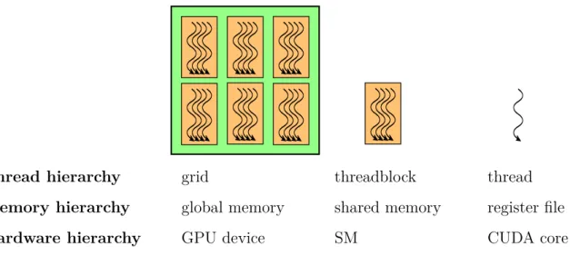
A summary of each component in the CUDA thread hierarchy and the corresponding level in the memory and hardware hierarchy is shown in Figure 2.1. Take note of the one-to-one correspondence between the components in the thread, memory, and hardware hierarchy.

CUDA uses the C++ programming language as a base, but extends it with concepts specific to GPUs. A simple kernel that adds two arrays A and B elementwise, and stores the result in a third array C is given in Listing 1. Note that the function VecAdd is annotated with the keyword__global__. These functions are executed on the GPU (also called device) rather than the CPU (also called host), and are commonly referred to as

(27)

Thread hierarchy Memory hierarchy Hardware hierarchy

grid threadblock thread

shared memory

global memory register file

GPU device SM CUDA core

Figure 2.1: An overview of each component in the CUDA thread hierarchy, along with the corresponding level in the memory and hardware hierarchy.

calling kernels will result in the creation of a set of N threads, each executing the same kernel in parallel. The example kernel is very simple: it accesses the identifier of the executing thread using the built-in threadIdx variable, and adds the elements in A and B at that position. Finally, on Line 10, this kernel is launched using the triple bracket syntax <<<M, N>>>, which starts the kernel with M blocks of N threads each.

2.2 The Julia programming language

Julia is an open source programming language featuring a high-level syntax, and per-formance on par with lower level languages such as C [25, 26]. In Julia, functions may have different behaviour depending on the exact types of the arguments [27]. In Julia parlance, each definition of such behaviour is referred to as a method. A central paradigm in the design of the language is the way it handles dispatch, the process by which the compiler determines which method to use for a given function call. Julia uses a multiple

dispatch scheme, which means that this choice depends on the number of arguments, and

(28)

1 __global__ void VecAdd(float* A, float* B, float* C) 2 {

3 int i = threadIdx.x;

4 C[i] = A[i] + B[i]; 5 } 6 7 int main() 8 { 9 // ... 10 VecAdd<<<1, N>>>(A, B, C); 11 // ... 12 }

Listing 1: A simple CUDA C++ kernel that adds two arrays elementwise. Adapted from the CUDA programming guide [52].

One feature of Julia’s type system is that it is parametric. This means that generic types may optionally be annotated with information through the use of type parameters. For example, we can parametrise the generic Array type to a parametric form Array{T}that

also includes the type of each element. Like most high-level programming languages, Julia’s type system is also dynamic, meaning that the types of expressions are not necessarily known at compile time. However, Julia also has some advantages of static type systems through several features of its compiler, which contrast it with the interpreters used in other high-level programming languages such as Python or R.

It achieves this through the combination of JIT (Just-In-Time) compilation, function specialisation, and type inference. Consider for example a simple Julia function that adds its two arguments: add(x, y) = x + y. In traditional dynamically typed languages, executing this function will involve a dynamic lookup of the types of x and y, and a dynamic call to the + operator corresponding to these types. The Julia compiler takes a different approach. Suppose we call this function using two 64-bit integers: add(1, 2). Through type inference, the compiler knows that both x and y are of type Int64. The

(29)

addfunction is then specialised for these argument types, and compiled just-in-time to an efficient implementation consisting of a simpleleaq (%rdi, %rsi), %rax on x86-64.

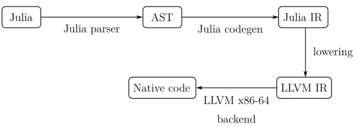
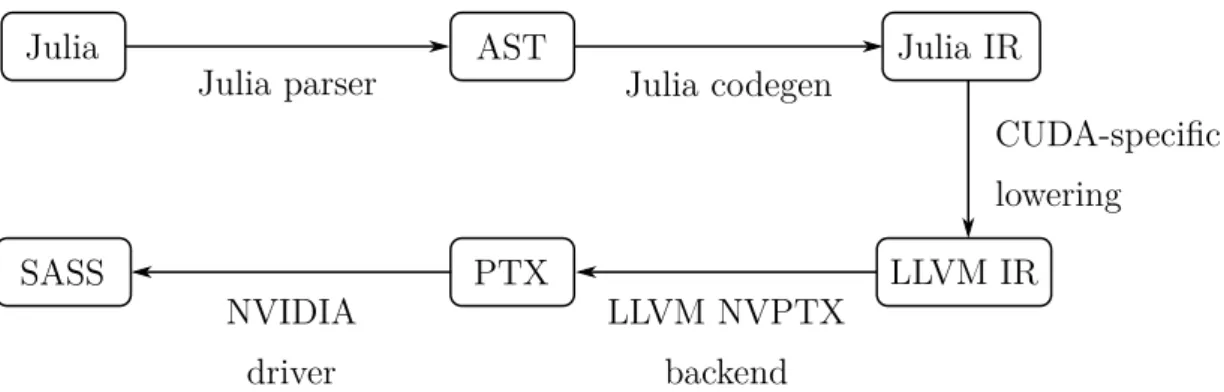
Julia’s compiler is built on top of LLVM, a compiler infrastructure project commonly used in research and industry [37]. The compilation process is illustrated in Figure 2.2. First, Julia code is parsed into an AST (Abstract Syntax Tree), a tree representation of the syntactical structure of the source code. This AST is then converted to a Julia-specific IR (Intermediate Representation), that is used for type inference. Next, Julia IR is lowered into the SSA (Static Single Assignment) form that LLVM uses, called LLVM IR. In the last step, this LLVM IR is then converted to native instructions by the LLVM backend corresponding to the current architecture, such as x86-64.

Julia AST Julia IR

LLVM IR Native code

Julia parser Julia codegen

lowering

LLVM x86-64 backend

Figure 2.2: An overview of the compilation pipeline of the Julia compiler.

Julia provides access to these intermediate representations from within the language itself. For example, Julia’s introspection capabilities include several macros that print the result of each step in the compilation pipeline. @code_loweredis used to display the Julia IR,

@code_typed and @code_warntype to display the lowered form after type inference. At a lower level,@code_llvm can be used to print the LLVM IR, and @code_native for the final machine code.

Apart from querying the intermediate representations, we can also change some of them within Julia. Similar to LISP, Julia represents the AST of parsed code as a data structure in the language itself, called an Expr. This is for example used to implement macros,

which return an Expr that is then compiled at parse time. More powerful is the concept

of generated functions, which, unlike macros, are expanded at a time when the types of the arguments are known. Like macros, generated functions return an that is

(30)

subsequently compiled. However, they can generate custom code for each combination of argument types.

Another way in which we can influence the compilation pipeline, is through the use of llvmcall. This function allows embedding LLVM IR directly into Julia source code. First, Julia determines the LLVM types corresponding to the Julia types of the arguments and return value, e.g. Julia’s Int64will be mapped to LLVM’s i64. Next, the compiler will generate an LLVM function with those types, containing the specified LLVM IR. As a last step, the llvmcall is replaced by a call to this function, and, if necessary, instructions to convert the arguments and return value to the correct LLVM type.

2.3 CUDAnative.jl: Executing Julia kernels on CUDA

hardware

CUDAnative.jl is a Julia package that allows executing kernels written in Julia on CUDA-enabled hardware [10]. To accomplish this, it uses the LLVM backend for NVIDIA GPUs, NVPTX, along with several features of the Julia programming language we have seen in Section 2.2. For example,llvmcallis used to call CUDA-specific LLVM instrinsics directly, as is the case for e.g. synchronising all threads in a threadblock.

Similarly, the CUDA memory hierarchy is exposed through the use of parametric types: CUDAnative’s type for device pointers,DevicePtr, has a parameter that determines the address space of the pointer, e.g. global or shared. When loading from or storing to this pointer, the multiple dispatch mechanism is used to dispatch to a custom implementation for device pointers. This implementation makes use of @generated functions to generate custom LLVM IR for each pointer type, and thus for each possible address space. Through the use of CUDAnative, one can replace C++ with Julia in the CUDA software stack. For example, Listing 2 shows the equivalent of the simple vector addition kernel of Listing 1. Kernels, such as vecadd, are regular Julia functions, that may

(31)

1 function vecadd(a, b, c) 2 i = threadIdx().x 3 c[i] = a[i] + b[i] 4 return

5 end 6

7 # ...

8 @cuda threads=N vecadd(a, b, c) 9 # ...

Listing 2: The CUDAnative.jl equivalent of the simple vector addition kernel in Listing 1. additionally contain CUDA-specific code, such as the call tothreadIdx()on Line 2. Note that kernels are only allowed to use a subset of the Julia language. Features that do not map well to GPUs, such as garbage collection and exceptions, are not supported. This kernel is then run on the device using the@cuda macro, which serves as a replacement of the triple bracket syntax of CUDA C++.

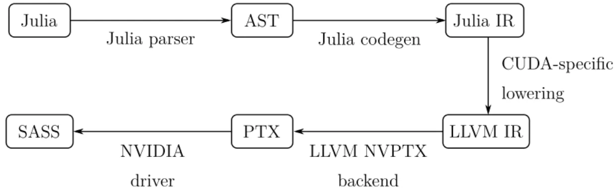
CUDAnative reuses part of the Julia compiler infrastructure we have seen in Figure 2.2. In particular, this compilation pipeline is run up until the lowering stage. The gener-ated code is then intercepted at the LLVM IR level, and sent to the LLVM NVPTX backend, instead of the backend corresponding to the host architecture. The adapted compilation pipeline is given in Figure 2.3. Note that, compared to the original pipeline, CUDAnative slightly changes the lowering process from Julia IR to LLVM IR.

Instead of x86-64 assembly instructions, the NVPTX backend emits PTX (Parallel Thread Execution) instructions. PTX is a low-level virtual ISA (Instruction Set Architecture), suitable for execution on CUDA-enabled NVIDIA GPUs. The main goal of PTX is to provide a stable ISA that is portable to different GPU architectures [60]. Note that this ISA is only virtual: for example, PTX uses an infinitely large set of virtual registers, that do not necessarily correspond to physical GPU registers. The GPU itself is not able to execute PTX directly. For this, the NVIDIA graphics driver contains a compiler that

(32)

translates this PTX into SASS (Streaming Assembler), the generation-specific ISA that the GPU uses.

Mimicking standard Julia’s introspection capabilities, CUDAnative also includes mac-ros that print the IRs of GPU kernels. These are named similarly to their Julia counterparts: it suffices to add a prefix device to their name, so that @code_llvm

becomes @device_code_llvm. CUDAnative also introduces @device_code_ptx and

@device_code_sassto inspect the generated PTX and SASS, respectively. These features are extremely useful to find out which instructions the LLVM backend or the CUDA driver generate for our kernels.

Julia AST Julia IR

LLVM IR Julia parser Julia codegen

CUDA-specific lowering LLVM NVPTX backend PTX SASS NVIDIA driver

Figure 2.3: An overview of Julia’s compilation pipeline adapted by CUDAnative.jl. Finally, we should briefly mention CuArrays.jl, a package built on top of CUDA-native.jl that defines a new array type, CuArray [12]. This package complements CUDAnative.jl by introducing several higher-level abstraction on top of the kernels generated by CUDAnative.jl. For example, the CuArray type implements Julia’s broadcast operation, which applies an operation elementwise. At the Julia language level, this is exposed using the special dot-syntax. As such, the vector addition from Listing 2 may be more succinctly written asc .= a .+ b, if all the given variables are of the type CuArray.

(33)

2.4 Mixed precision arithmetic

While FP64 (Double Precision Floating Point) arithmetic has long been the de facto standard in the domain of scientific computing, mixed precision arithmetic is quickly gaining traction [16]. This new concept originated in the fields of ML and DL (Deep Learning), where numerical accuracy is of lesser importance than performance. Clearly, as long as the neural network converges to a model of similar accuracy, it does not matter that intermediate computations have reduced accuracy. Performance, on the other hand, is pivotal: the training and inference process is repeated for each batch of input samples, and for each choice of the hyperparameters of the model.

Mixed precision is, as its name suggests, the process of combining two precisions: FP32 (Single Precision Floating Point) and FP16 (Half Precision Floating Point). The general idea is to perform the main computations in FP16, but store a minimal amount of information in FP32, which is important to guarantee convergence of neural networks. There are several advantages to using mixed precision, compared to the traditional FP64 or FP32 approach [50]:

1. Power consumption: Hardware implementing mixed precision arithmetic tends to consume less power than traditional FPUs (Floating Point Units) for FP32 or FP64.

2. Computation time: For workloads that are mainly compute-bound, mixed precision will increase performance, since they are typically faster than full FP32.

3. Memory bandwidth: Since FP16 are only 2 bytes long compared to FP32’s 4 bytes, the required memory bandwidth to load/store them is twice as small, which is beneficial for memory-bound tasks.

4. Memory usage: Similarly, an array of FP16 elements will only require half as much storage in global memory. In the context of neural networks, this means that we can double the batch size used during training.

(34)

It has been demonstrated that mixed precision models are able to achieve the same accuracy as their full precision counterparts [44]. What makes this even more remarkable is the fact that this can be accomplished without any changes to the model architecture or hyperparameters. Through the use of techniques such as gradient scaling and maintaining a single-precision copy of the weights, this holds true for a variety of different ML models. Compared to ML, HPC applications are much more sensitive to the precision loss induced by the use of mixed precision. However, it is possible to limit this loss in precision using precision refinement techniques [41]. Consider the case of the multiplication of two matrices AFP32 and BFP32, initially stored in FP32. We convert each of these to FP16, and calculate the residual matrices Ares = AFP32− AFP16 and Bres = BFP32− BFP16. We can then obtain a higher precision result using four mixed-precision multiplications as AFP32BFP32 = AFP16BFP16+ AFP16Bres+ AresBFP16+ AresBres. This scheme can be improved by applying the refinement iteratively. Such iterative refinement techniques have already proven their use in mixed-precision solvers for linear systems [17].

Since ML and DL typically use GPUs, it was only a matter of time before NVIDIA saw the importance of supporting mixed precision. In 2017, NVIDIA first incorporated mixed precision in their Volta-generation GPUs. This GPU generation introduced Tensor Cores, a new type of processing core specifically designed for mixed precision arithmetic [5]. In terms of the traditional GPU hardware hierarchy, we may think of them as being “inside of the CUDA cores”, complementing the traditional FPU that performs FP32 operations. Tensor Cores of the Volta generation perform a 4 × 4 × 4 matrix MAC (Multiply Accumulate) operation, i.e. an operation of the form D = A · B + C, where

A, B, C and D are 4 × 4 matrices. This MAC operation is performed in mixed precision,

meaning that the input matrices A and B are stored in FP16, whereas the accumulation matrices C and D may be either FP16 or FP32.

The second generation Tensor Cores were introduced in 2018 with the launch of NVIDIA’s Turing architecture [57]. Turing Tensor Cores extend the first generation Tensor Cores with support for 8-bit, 4-bit, and 1-bit integer data types. These are useful for ML workloads that are more tolerant to precision loss, and do not require the full 16-bit precision of FP16.

(35)

On 14 May 2020, NVIDIA presented the Ampere GPU architecture, and the new NVIDIA A100 GPU [34]. The A100 includes the third generation Tensor Cores, which support all the operations of Volta’s and Turing’s Tensor Cores, and additionally add new capabilities. Tensor Cores of the Ampere generation support FP64, which is useful for HPC applications, and BF16 (Bfloat16), a truncated version of the IEEE FP32 format. Ampere Tensor Cores also implement operations in a newly introduced floating point format, TF32 (TensorFloat-32), a hybrid of the standardised FP16 and FP32 formats. Like FP16, TF32 uses a 10-bit mantissa, since that is typically sufficient for the precision requirements of ML applications. The main limitation of FP16 is that the numeric range is quite limited, since it only has 5 bits allocated to the exponent. For that reason, TF32 uses the same 8-bit exponent that is used for FP32, so that the same range is supported.

(36)

3 Motivation and related work

In this chapter, we will focus on matrix multiplication. To start off, we explain why we are interested in matrix multiplication kernels in the first place. Next, we illustrate why there is a need for flexiblity in matrix multiplication kernels, and argue that the current state-of-the-art is lacking in this respect. Finally, we conclude by summarising the main goals of this thesis, and how each of these is mapped to the remaining chapters.

3.1 The case for matrix multiplication

Matrix multiplication kernels are interesting for several reasons. First, matrix multi-plication is one of the most common operations in linear algebra. This is evidenced by the fact that matrix multiplication is standardised in the BLAS (Basic Linear Algebra Subprograms) specification, a collection of low-level computational routines that has evolved into a de facto standard [14]. BLAS functionality is separated in three separate categories, called levels: vector-vector operations (BLAS level 1), matrix-vector opera-tions (BLAS level 2), and matrix-matrix operaopera-tions (BLAS level 3). In this work, we are mainly interested in BLAS level 3, and more specifically, in its GEMM routine, which calculates a scaled matrix MAC, i.e. an expression of the form D = αA · B + βC. Because GEMM is a matrix-matrix operation, there are many opportunities to improve performance by exploiting memory locality. Consider for example a GEMM where all matrices have size N × N. In this case, one matrix contains N2 elements, leading to a total memory consumption of O(N2). Each of the N2 elements of the output requires N