Ecological effects of pesticide use in the Netherlands: Modeled and observed effects in the field ditch

(1)

Ecological effects of pesticide use in the Netherlands

Modeled and observed effects in the field ditch D. de Zwart

This investigation has been performed by order and for the account of the Ministry of Spatial Planning, Housing and the Environment, within the framework of project M/500002,

“Modeling ecological effects”.

(2)

(3)

Abstract

This study dealing with risks to the aquatic ecosystem imposed by the application of

pesticides in the Netherlands made use of a novel method to calculate aquatic exposure to a large variety of pesticides (261 in total), which is worked out in detail here. Since the entire calculation is founded on GIS-based maps of agricultural land use (51 crops in open culture), it is possible to generate country-wide maps of the results. Through the application of

Sensitivity Distributions for aquatic species (SSD), in combination with rules for mixture toxicity calculation, the modeled exposure is transformed to a risk estimate for the species assemblage in the aquatic ecosystem. The risk is expressed as the proportion of species likely to be suffering any effect from the exposure. In the summary of the risk maps, the majority of predicted effects is observed to be caused by the pesticide application practice in growing potato crops: 95% of the predicted risk is caused by only 7 of the 261 pesticide ingredients. The maximum local risk of pesticide use is estimated to affect about 50% of species. For the purpose of validation, local toxic risk estimates were compared to observed species

composition in field ditches using simple statistical methods (regression analysis). However, the number of field observations was not sufficient enough to generate quantitative results. The unexplained variability in the biotic field data collected by a range of non-aligned monitoring networks does not allow highly significant conclusions. Nevertheless, there is a weak indication that the predicted risks are associated to biodiversity changes in field-exposed communities.

(4)

(5)

Samenvatting

Deze studie toont aan dat het mogelijk is om het ecotoxicologische risico te berekenen van het gebruik van bestrijdingsmiddelen in de Nederlandse landbouw, en dat deze berekende risicowaarden betekenisvol zijn in het licht van waarneembare effecten. Voor de

riscoberekening is uitgegaan van het agrarisch bodemgebruik in het jaar 1998. De

51 verschillende teeltgewassen, die in de open lucht gekweekt worden, kennen alle een eigen standaard regiem van bestrijdingsmiddelengebruik. In totaal worden in de open teelt van landbouwgewassen 261 verschillende werkzame stoffen (ingrediënten van

bestrijdingsmiddelen) toegepast. In een waterrijk land als Nederland is het waarschijnlijk dat een aanzienlijk deel van de gebruikte bestrijdingsmiddelen onbedoeld in het oppervlaktewater terechtkomt. De blootstelling van het oppervlaktewater is berekend, waarbij de volgende processen in beschouwing werden genomen:

• Direct transport van spuitnevel naar kavelsloten;

• Droge depositie van gasvormige bestrijdingsmiddelen in sloten; • Natte depositie van bestrijdingsmiddelen door uitregenen in sloten; • Afstroom- en drainagewater dat van het veld de sloot in loopt; • Adsorptie van bestrijdingsmiddelen aan bodemmateriaal; • Afbraak van bestrijdingsmiddelen in sloot en bodem.

De berekende aquatische blootstelling aan bestrijdingsmiddelen wordt met behulp van de verdeling van de gevoeligheid over soorten waterorganismen en regels voor

combinatietoxiciteit omgezet in een maat voor het ecotoxicologische risico. Dit risico wordt uitgedrukt als de fractie van de soorten die geacht worden te zijn blootgesteld aan een concentratie of mengselconcentratie die uitgaat boven het niveau waarop geen effecten meer optreden.

De diverse berekeningen zijn per gridcel van 500 x 500 meter uitgevoerd voor het hele droge areaal van Nederland. Het maximum risico dat voor enige gridcel in NL is berekend bedraagt 51%. Het risico komt, omvang en oppervlakte gewogen, voor 58% voor rekening van de aardappelteelt. Slechts 7 van de 261 stoffen dragen voor 95% bij aan het berekende risico. Van deze 95% nemen 2 verschillende fungiciden met 60% het leeuwendeel voor hun rekening. Een drietal insecticiden draagt voor 29% bij aan het risico, terwijl de resterende twee herbiciden voor 7% van het risico verantwoordelijk zijn.

Het risico, in termen van de potentieel aangetaste fractie van de soorten, is vergeleken met de door waterkwaliteitsbeheerders gemeten soortensamenstelling van macrofauna en

waterplanten in sloten. Ondanks de beperkte beschikbaarheid van waarnemingen en een grote mate van onverklaarde variabiliteit in de dataset, is er een zwakke indicatie dat het berekende risico gerelateerd is aan een verarming van de macrofauna soortensamenstelling in het veld.

(8)

Voor de waterplanten is een dergelijke relatie niet aantoonbaar, hetgeen vermoedelijk wordt veroorzaak door het geringe aandeel van de herbiciden aan het berekende risico.

(9)

Summary

This study demonstrates that it is possible to calculate the ecotoxic risk associated with the use of pesticides. This risk estimate is calculated from the agricultural landuse map of the Netherlands for the year 1998. The 51 different open air cultured crops all have a standard regimen of pesticide application. It total 261 active substances are used as pesticide ingredients. In a flat and wet country, like the Netherlands, it is highly likely that a

considerable proportion of the applied pesticides is transferred to surface water. The exposure of surface water (adjacent field ditches) is calculated, taking the following processes into account:

• Direct spray drift;

• Dry deposition of airborne pesticides;

• Direct rain deposition of airborne pesticides in ditches;

• Run-off and drainage from the crop field to adjacent surface water; • Adsorption to soil particulates and soil organic matter;

• Degradation in soil and surface water.

The calculated exposure of the field ditch is converted to the estimate of risk by applying species sensitivity distributions and theory on mixture toxicity. The risk is expressed in terms of the fraction of species that is expected to be exposed to concentrations or mixture

concentrations exceeding the levels where effects are considered negligible.

All the calculations are performed per gridcell of 500-meter square for the entire dry area of the Netherlands. The maximum risk calculated for any gridcell mounts up to 51%. Risk and area-wise, 58% of the risk can be attributed to the culture of potato crops. If the exposed area is also taken into account, only 7 out of 261 pesticide ingredients contribute to 95% of the risk. The 95% contribution to the overall risk can be attributed to two different fungicides (60%), 3 insecticides (29%) and 2 herbicides (7%).

The calculated risk in terms of the potentially affected fraction of species is compared to measured data on the species composition in field ditches. Despite the few observations available, that are also of relatively poor quality, there is a weak indication that the predicted risk is reflected in a comparable reduction in the diversity of macrofauna species. For the macrophytes this phenomenon could not be detected, most probably due to the small contribution of herbicides to the overall risk.

(10)

(11)

1. Introduction

1.1 Problem definition

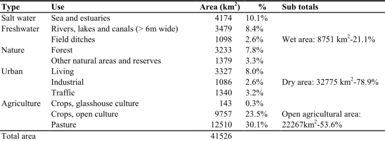
The Netherlands is a small country with a very intense agricultural practice. Table 1 shows the landuse pattern for the Netherlands in the year 1998. Of the total dry surface area of about 32500 km2, about 22000 km2 is dedicated towards open use for culturing crops and feeding cattle. In 1998, a total amount of 6.5 million kg of a variety of 261 different active pesticide ingredients was applied to grass and crop lands together. The Netherlands is also a very flat, low-lying country. About half the country is about level with the sea. Without dunes and water barriers, more than half of the Netherlands would be flooded. The highest point is only 300 m above sea level. Therefore, the agricultural land is drained by an extensive system of man-made ditches. The ditches are connected to canals, from where the excess water is pumped to rivers and eventually to the sea. In the lower regions of the country, the ditches form a network with an interdistance of between 25 and 100 meters. The many dykes, locks, pumping stations, flood barriers, canals and ditches keep the Netherlands habitable.

Table 1 Land use pattern in the Netherlands for 1998, (modified after CBS, http://statline.cbs.nl/, September 2003).

Type Use Area (km2) % Sub totals

Salt water Sea and estuaries 4174 10.1%

Freshwater Rivers, lakes and canals (> 6m wide) 3479 8.4%

Field ditches 1098 2.6% Wet area: 8751 km2_-21.1%

Nature Forest 3233 7.8%

Other natural areas and reserves 1379 3.3%

Urban Living 3327 8.0%

Industrial 1086 2.6% Dry area: 32775 km2_-78.9%

Traffic 1340 3.2%

Agriculture Crops, glasshouse culture 143 0.3%

Crops, open culture 9757 23.5% Open agricultural area:

Pasture 12510 30.1% 22267km2_-53.6%

Total area 41526

Due to these geographical conditions, it is very likely that a considerable proportion of the pesticides applied to agricultural land is unintendedly transferred to the water in the field ditches. The question is, whether this unintended exposure bears risks for the aquatic community.

1.2 Towards quantification of risks

With the input of the type and area of 51 different crops grown in the open air (including grass land) for about 120,000 gridcells of 500 * 500 m, together with a standard weekly agricultural regimen in applying pesticides to those crops, a GIS-based (Geographical Information System) estimate of pesticide concentrations in those ditches is generated.

(12)

Exposure pathways and processes incorporated in the calculations of water concentrations include:

1. Aquatic exposure by direct spray drift; 2. Run-off and drainage from the soil (R&D); 3. Wet and dry deposition for airborne pesticides; 4. Sorption to soil particulates;

5. Leaching to deeper groundwater; 6. Degradation in soil and water.

By using sensitivity distributions for aquatic species, together with criteria for mixture

toxicity evaluation (Posthuma et al., 2002), the calculated concentrations are transformed into an ecotoxic risk estimate for the aquatic community, that is also GIS-based. The risk is expressed as the multi-substance Potentially Affected Fraction of species (msPAF), that is defined as the proportion of species exposed to a mixture of pesticide concentrations exceeding their respective Predicted No Effect Concentration (PNEC).

Local and regional water management in the Netherlands is in the hands of regional Water Authorities. The Water Boards are responsible for flood control, water quantity, water quality and treatment of urban wastewater. All of the about 35 Water Boards do operate a monitoring network. Concentration of pollutants and classical water quality variables are regularly measured in combination with the occurrence of aquatic species. Though very elaborately quantified, the measured concentrations of pesticides (about 500,000 records over the past 10 years) do not reflect actual aquatic exposure. This has been concluded in a qualitative pilot study performed in 1999 (not reported). Lack of realism in measured pesticide concentrations may in part be due to the fact that the sampling schemes are not adjusted to the regimen of pesticide application. There may also be regional discrepancies between the types of pesticide measured and the types of pesticide used. Furthermore, lack of realism may be caused by analytical difficulties in quantifying low concentrations of pesticides in the medium “surface water”.

Calculating the aquatic exposure concentrations from the types of crops locally grown has the advantage that the modeled effects can locally be attributed to the types of crops, as well as to the types of pesticides. This enables us to conduct scenario studies that can guide policy decisions in spatial planning and in pesticide regulation.

1.3 Aims

In this report it is tried to:

1. Calculate concentrations from the use of pesticides and compound behavior; 2. Calculate the ecotoxic risk per compound and for the mixture as a whole;

3. Associate calculated risks with pesticides, crops and observed species occurrence in the field.

(13)

2. Available data

2.1 Data on active pesticide ingredients

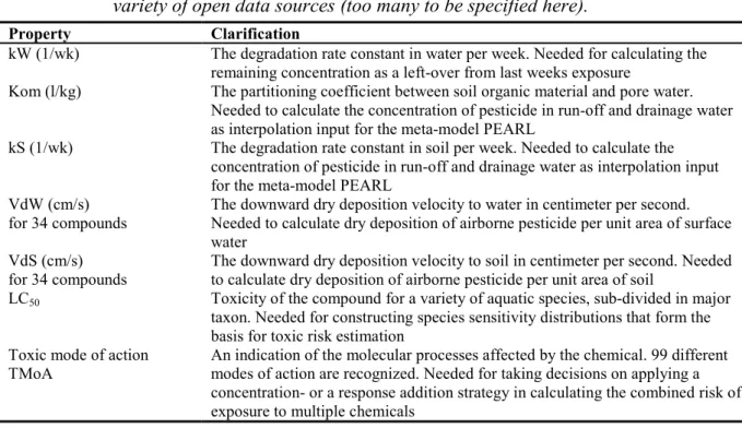
In this study a total of 261 active pesticide ingredients is evaluated (Appendix 1). For all of those chemicals it was possible to generate estimates of the properties presented in Table 2 by consulting open literature and the internet, as well as by querying publicly available databases on chemical properties.

Table 2 Chemical properties of active pesticide ingredients gathered from a large variety of open data sources (too many to be specified here).

Property Clarification

kW (1/wk) The degradation rate constant in water per week. Needed for calculating the remaining concentration as a left-over from last weeks exposure

Kom (l/kg) The partitioning coefficient between soil organic material and pore water. Needed to calculate the concentration of pesticide in run-off and drainage water as interpolation input for the meta-model PEARL

kS (1/wk) The degradation rate constant in soil per week. Needed to calculate the concentration of pesticide in run-off and drainage water as interpolation input for the meta-model PEARL

VdW (cm/s)

for 34 compounds The downward dry deposition velocity to water in centimeter per second.Needed to calculate dry deposition of airborne pesticide per unit area of surface water

VdS (cm/s)

for 34 compounds The downward dry deposition velocity to soil in centimeter per second. Neededto calculate dry deposition of airborne pesticide per unit area of soil LC50 Toxicity of the compound for a variety of aquatic species, sub-divided in major

taxon. Needed for constructing species sensitivity distributions that form the basis for toxic risk estimation

Toxic mode of action

TMoA An indication of the molecular processes affected by the chemical. 99 differentmodes of action are recognized. Needed for taking decisions on applying a concentration- or a response addition strategy in calculating the combined risk of exposure to multiple chemicals

2.2 Grid-based soil properties

From the 500-m square gridcell-based soil map of the Netherlands (De Vries and Denneboom, 1992), a number of soil properties were extracted as presented in Table 3.

Table 3 Soil properties in the Netherlands.

Property Clarification

fom The fraction of organic matter in the soil. Needed to calculate the concentration

of pesticide in run-off and drainage water as interpolation input for the meta-model PEARL

fwater The fraction of surface water per gridcell. Needed to calculate the additional

effect of exposure to the pesticide content in drainage and run-off water Soil permeability (m/d) The leeching velocity of water in soil in meters per day. Needed to calculate the

(14)

2.3 Climatic data

Over the years 2000-2001, TNO operated a monitoring program, quantifying the amount of deposition (mm) at 18 stations in the Netherlands per period of 4 weeks (TNO, 2002). The measured amounts of deposition were converted to nation-wide 10-km square gridcell-based maps of 4-week average deposition by applying kriging interpolation. The weekly amount of rain is calculated as ¼ of the 4-weekly amount.

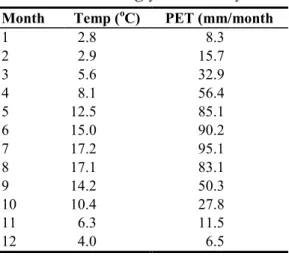
Daily average temperature data over the period 1991-2000 (file: etmgeg_260_1991.gz) were obtained from KNMI (www.knmi.nl/product, September 2003). Weekly potential

evapotranspiration (PET) was calculated from the 10-year series of daily average temperature values, using the relationship between T and PET from the 30-year monthly averages given in Table 4.

Table 4: Long-year monthly average of temperature and potential evapotranspiration.

Month Temp (oC) PET (mm/month

1 2.8 8.3 2 2.9 15.7 3 5.6 32.9 4 8.1 56.4 5 12.5 85.1 6 15.0 90.2 7 17.2 95.1 8 17.1 83.1 9 14.2 50.3 10 10.4 27.8 11 6.3 11.5 12 4.0 6.5

2.4 Land use and Crops

Geographical land use data were obtained from a database on land use based on satellite images of the years 1999 and 2000 (LGN4; http://www.lgn.nl/, September 2003). The land use data were combined with the 1998 crop areas from the Agricultural Economics Research Institute (LEI-DLO, BedrijvenInformatieNet, http://www.lei.dlo.nl/home.htm, September 2003). These crop areas were available for 540 out of 548 municipalities in the Netherlands. The crop definitions for 1998 are based on a classification system of Statistics Netherlands

(http://statline.cbs.nl/, September 2003).

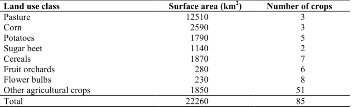
Clustering the non-agricultural land use into the land use types urban area, nature area, and open water area reduced the number of land use classes in LGN4. These 3 land use types were combined with the 9 agricultural classes of LGN4 (pasture, corn, potatoes, sugar beet, cereals, greenhouses, fruit orchards, flower bulbs, and other agricultural crops). The land use data were aggregated to the scale level of gridcells of 500 m by 500 m, by calculating the distribution of the land use classes from the 400 pixels within each gridcell. The national acreage of the 8 open-air agricultural land use classes is shown in table 5.

(15)

Table 5: Land use classes; national acreage and open air crop distribution for the year 1998, based on LGN4.

Land use class Surface area (km2₎ _{Number of crops}

Pasture 12510 3 Corn 2590 3 Potatoes 1790 5 Sugar beet 1140 2 Cereals 1870 7 Fruit orchards 280 6 Flower bulbs 230 8

Other agricultural crops 1850 51

Total 22260 85

In order to relate pesticide application data to open air land use, the 85 crop types were distributed among the agricultural land use classes. The largest number of crops was assigned to the land use class that contains other types of agricultural crops. The procedure for

calculating the spatial distribution of crop areas among the gridcells uses the land use class area and the crop area expressed as a fraction of the total area of land use class.

CAGC,CR = LUARGC,LU • CRARMU,CR / LUARMUMU,LU

where,

CAGC,CR the gridcell-based crop area (ha)

LUARGC,LU the gridcell-based land use class area (ha)

CRARMU,CR the municipality-based crop area (ha)

LUARMUMU,LU the land use area in all gridcells of a municipality (ha)

This procedure generated estimated open-air crop areas for 51 out of 85 crops on a total of 122259 gridcells of 500 x 500 m square. The 51 different crops are given in table 6.

Table 6: Crops quantified.

Crop name Crop name Crop name

Strawberry Gladiolus Leek

Apple, young Grass seed Rose

Apple, old Hyacinth Oyster plant

Asparagus Iris Conifer

Cabbage storable Marrowfat pea Headed cabbage

Permanent pasture Corn Fodder maize

Hedge plants Park trees Sprout cabbage

Brown beans Lily Dwarf bean

Chicory root Daffodil Sugar beet

Potato on clay Other flowers Temporary pasture

Potato, other Pear, young Tulip

Corn-cob-mix Pear, old Perennial garden plants

Flowers to be dried Plant onion Field bean Green peas Plant potato on clay Other fruit tree Starch potato Plant potato, other Small carrot

Summer barley Winter wheat Winter carrot

(16)

2.5 Application regimen of pesticide ingredients per crop

For 51 of the 85 open-air crops, the total national use in 1998 of 261 active pesticide ingredients was available per week (http://statline.cbs.nl/, September 2003). The data were kindly provided by a query from the Informatie Systeem Bestrijdingsmiddelen (ISBEST 4.0) conducted by Alterra. This information together with the estimated gridcell-based crop area generates the estimated weekly gridcell-based use of active ingredients.

2.6 Direct spray drift of pesticide ingredients to a field ditch

Per crop and per active ingredient, the direct spray drift to a standardized adjacent field ditch is given by ISBEST 4.0 (kindly received from Alterra). The drift given by ISBEST is

expressed as the percentage of the applied dose (kg/gridcell) transferred to a hectare of surface water ([Drift (%Dose)]).

2.7 Direct transfer of pesticide ingredients to the soil

Based on the application data for the individual pesticide ingredients per week, per crop and per gridcell, together with chemical properties, ISBEST 4.0 generated data on the average fraction of the ingredients transferred to the soil ([SDvsUse]).

2.8 Pesticide ingredients in air and wet precipitation

Over the years 2000-2001, TNO operated a monitoring program, quantifying the amount of pesticide ingredients in air and deposition at 18 stations in the Netherlands (TNO, 2002). 34 pesticide ingredients were selected for this monitoring program by virtue of their ability to evaporate and get airborne. Both the air and deposition quantities of pesticides were

converted to nation-wide 10-km square gridcell-based maps by applying kriging interpolation. The concentration in air was expressed in ng/m3, averaged over a 4-week period. The quantity of pesticide constituents in rainwater was given as a load expressed in grams per hectare per 4-week period. Divided by 4 this yielded the estimated weekly load (g/ha/wk), as used in the current analysis.

2.9 Pesticide concentration in run-off and drainage water

The model “PEARL” (Leistra et al., 2000) generated a table giving the pesticide

concentrations in run-off and drainage water (pore water) after application of 1 kg per hectare as a function of two chemical properties of a range of imaginary pesticides:

(17)

2. Partitioning between soil organic matter and pore water (Kom * fom), ranging between 0

and 200 (l/kg). The table is generated under the assumption that the soil contains 4.7 percent of organic matter.

2.10 Chemical and species monitoring data in ditches

For the year 1998, the Water Boards operated an ecological monitoring network that provided species census data for 257 field ditches in the Netherlands where macrofauna and

macrophyte data were collected. The data were retrieved from the Limnodata Neerlandica database, kindly received from Royal Haskoning (Status: April 17th, 2003). The database comprised counts of 1007 macrofauna and 291 macrophyte taxa. Removing extremely scarce species, a total of 344 macrofauna and 113 macrophyte taxa were retained. If a station was evaluated two or more times during the year 1998, the maximum count per taxon was used. The taxa comprised individual species, as well as higher taxonomic levels. For ease of language, the term “species” will be used for all taxonomical entities.

The biological dataset was matched by a chemical dataset for 212 out of 257 stations. The dataset was comprised of data on the local concentrations of Chloride, Total phosphorus, Kjeldahl Nitrogen, Dissolved Oxygen and pH. If the stations were visited several times over the year 1998, the average was taken over the number of observations.

(18)

(19)

3. Methods for calculating exposure

3.1 Exposure assumptions and data storage

In order to simplify the exposure calculations, the following assumptions were made: 1. All calculations are performed for a standardized ditch. A standard ditch is assumed to

have an overall width of 1 m and a depth of 0.30 m, with sides sloping 45 degrees. One meter of standard ditch thus has a water content of 210 liters.

2. All fluxes of pesticide input to the ditches are weekly assumed to take place at a single moment in time.

3. The surface water in the ditches is assumed to be completely stagnant, despite the input of rain and drainage water.

4. All calculations, including the risk estimation, are performed one gridcell at a time, without taking influences of adjacent gridcells into account.

• Intermediate results are stored in a temporary database, being discarded after a round of single gridcell calculations.

• Temporary and permanent database entities are represented by field codes between brackets [...].

3.2 Start of the exposure and risk calculation process for a

single gridcell

3.2.1 Amount of precipitation transferred to ditch and soil

Using the TNO precipitation data, the direct rain input per week is calculated according to: [Amount of rain transferred to ditches (l/l/wk)] = [Amount of Deposition (mm/wk)] / 210 [Amount of rain transferred to the soil (l/m2/wk)] = [Amount of Deposition (mm/wk)]

3.2.2 Concentration of pesticide ingredients in rain water

Using TNO data per week and per pesticide ingredient, the concentration of 34 pesticide ingredients in rainwater is calculated:

[Concentration of pesticide ingredients in rain (µg/l)] =

(20)

3.2.3 Aquatic exposure by direct spray drift

Using crop area per gridcell in relation to the national crop area and the national use of ingredients, together with the drift percentage, the aquatic drift exposure per active ingredient and per gridcell is calculated by the following formula. Since only half of the ditches are located downwind of the application field, the calculated drift input is divided by 2: [Drift exposure in ditch (µg/l/wk)] =

Sum over all crops in gridcell([CropAreaGridcell (ha)] / [TotalCropAreaNL (ha)] * [UseCropNLperWeek (kg)] * [Drift (%Dose)]) * 10^9 (kg to µg) / 2100000 (ha ditch to l water / 2 (only downwind ditches)

3.2.4 Aquatic exposure by dry deposition

Using the (TNO-derived) 4-week maps of average concentration of 34 pesticides ingredients in air, together with the downward dry deposition velocity to water in centimeter per second, the dry deposition exposure to the standard ditch was calculated per gridcell and per

ingredient:

[Dry deposition exposure in ditch (µg/l/wk)] =

[AirConcentration (ng/m3)] / 1000 * 7*24*60*60 * [VdW (cm/s)] / 100 / 210

3.2.5 Soil loading by application of pesticides, A

Using crop area per gridcell in relation to the national crop area and the national use of ingredients, together with the soil transfer fraction, the soil loading in kg of active ingredient per hectare was calculated by the following formula, where the soil surface area treated is corrected for the area of surface water per gridcell:

[Soil transfer by use (kg/ha/wk)] =

Sum over all crops in gridcell([CropAreaGridcell (ha)] / [TotalCropAreaNL (ha)] * [UseCropNLperWeek (kg)] * [SDvsUse]) / (25 * (1- [fwater]))

3.2.6 Soil loading by dry deposition of pesticide ingredients, B

Using the (TNO derived) 4-week maps of average concentration of 34 pesticides ingredients in air, together with the downward dry deposition velocity to soil in centimeter per second, the weekly dry deposition exposure on soil was calculated:

[Dry deposition on soil (kg/ha/wk)] =

(21)

3.2.7 Soil loading of pesticide ingredients by rain input, C

Using TNO-data, the wet loading of pesticides to soil can be calculated: [Wet deposition on soil (kg/ha/wk)] =

[RainLoad (g/ha/wk)] / 103

3.2.8 Total loading of soil

Per pesticide ingredient and per gridcell, the total loading of the soil (kg/ha/wk) is the sum of the three soil loadings A, B and C.

[TotalSoilLoad (kg/ha/wk)] = A + B + C

3.2.9 Concentration in run-off and drainage water

The meta-model “PEARL”, the Kom partitioning coefficient of the pesticide and the soil organic fraction were used to calculate the concentration of pesticides in run-off and drainage water (R&D).

DT50(d) in soil can be calculated from the degradation rate constant, [kS (1/wk)]: • Ct = Co*e-kS*t(wk)

• Ct/Co = e-kS*t(wk)

• ln(0.5)= -[kS (1/wk)]*DT50(wk) • DT50(wk) = -ln(0.5)/ [kS (1/wk)]

• DT50 (d) = DT50(wk)*7 = 4.852 * [kS (1/wk)]

The actual partitioning in the field requires a correction for the local fraction of organic matter:

• K* = [Kom] * [fom, gridcell]/0.047

To calculate the concentration of a particular pesticide in R&D-water [Concentration in R&D (µg/l)], the “PEARL”-table is interpolated with the actual pesticide specific values of

DT50(d) and K*. The result is subsequently multiplied by the total soil loading of the pesticide ingredient [TotalSoilLoad (kg/ha/wk)] for the gridcell.

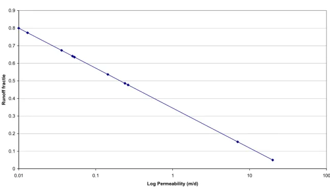
3.2.10 Amount of R&D water transferred to ditch

According to Meinardi and Schotten (in prep.), the fraction of precipitation surplus (precipitation – potental evapotranspiration) that is transferred to surface water by R&D-water is related to soil permeability. The empirically derived relationship is given in Figure 1.

(22)

Permeability vs Runoff fraction 0 0.1 0.2 0.3 0.4 0.5 0.6 0.7 0.8 0.9 0.01 0.1 1 10 100 Log Permeability (m/d) R unoff fr a c tie

Figure 1 The relationship of log(permeability) in m/day versus run-off and drainage fraction.

TNO-derived precipitation is expressed in mm/wk, which is equal to l/m2/wk. The volume of R&D-water received per liter of water in the ditches is calculated according to the following formula, where the ratio between the wet and the dry surface area is taken into account: [Amount of R&D (l/l ditch/wk)] =

([Amount of Deposition (mm/wk)]-[PET (mm/wk)]) * [R&DFraction] * (1- [fwater])/ [fwater] /

210

3.2.11 Iteration of the weekly concentration in ditch water

All the above calculations are performed for a single gridcell at a time, for all 261 pesticide ingredients and for all 52 weeks in the year. The results are stored in a temporary database that is discarded as soon as the toxic risk is calculated.

Per ingredient, the iteration starts with calculating the concentration that is left over from last week’s final concentration after one week of degradation in the water of the ditch:

[Present week’s start concentration (µg/l)] = Past weeks [Present week’s final concentration (µg/l)] * e –[kW(1/wk)]

Subsequently, the drifted and the dryly-deposited concentrations are added to the start concentration to form a [Sub-total concentration (µg/l)] after “dry addition”.

(23)

The final concentration for the present week is calculated by adding the water contained pesticide input from rain and run-off and drainage, with a correction for volume change: [Present week’s final concentration (µg/l)] =

([Sub-total concentration (µg/l)] *1 +

+ [Amount of rain transferred to ditches (l/l/wk)] * [Concentration in rain (µg/l)] + + [Amount of R&D (l/l ditch/wk)] * [Concentration in R&D (µg/l)]) /

(1 + [Amount of rain transferred to ditches (l/l/wk)] + [Amount of R&D (l/l ditch/wk)]) Furthermore, the weekly individual pesticide load is attributed to the origin of the exposure in terms of percentages of pesticide originating from past week exposure (old), drift exposure (drift), dry deposition (dry), wet deposition (wet) and R&D, respectively.

Per week and per pesticide, the [Present weeks final concentration (µg/l)], as well as the contributing loading percentages ([Old%], [Drift%], [Dry%], [Wet%] and [R&D%]) are stored in the temporary database.

In order to stabilize the concentration of pesticide ingredients remaining from past week, this iteration loop is continued for 5 times 52 weeks (5 years). The first week of the first year, the final concentration from past week is set to 0. The first week of the second year, the final concentration from past week is set to the final concentration of the last week of the first year, etc.

3.3 Gridcell-based concentration results

This final calculation in the exposure assessment yielded weekly concentrations of the 261 pesticide ingredients in field ditches, together with the percentages of load origin per gridcell. Without proceeding to the next gridcell, the calculated data were handed over to the routine for risk calculation. Only after finalizing the risk calculation routine, the concentration calculation routine is repeated for the next gridcell.

(24)

(25)

4. Methods for calculating toxic risk for aquatic

species

4.1 The method of toxic risk calculation

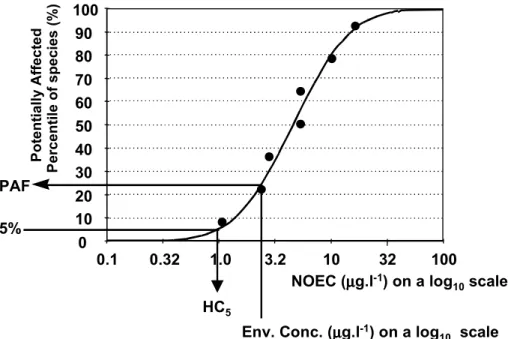
Toxic risk is calculated by the Species Sensitivity Distribution (SSD) methodology (Posthuma et al., 2002). An SSD-curve (Figure 2) is a cumulative distribution function of laboratory derived toxicity data for a single toxicant. SSD-curves are used to derive

Environmental Quality Criteria (EQC) and to quantify ecotoxicological risk. As an EQC, the Hazard Concentration for 5% of the species (HC5) predicts an environmental concentration

below which only an acceptably small proportion of species (5%) would be affected. As a risk estimate, the SSD is used to predict the proportion of species exposed to a concentration generating some kind of effect (the Potentially Affected Fraction: PAF). In the present study, the SSD-curves are assumed to follow a log-normal distribution.

0 10 20 30 40 50 60 70 80 90 100 0.1 0.32 1.0 3.2 10 32 100 NOEC (µµµµg.l-1_{) on a log} 10 scale PAF

Env. Conc. (µµµµg.l-1_{) on a log}

10 scale P o te nt ially A ff ec te d P erc ent ile of spe cies ( % ) 5% HC5

Figure 2 Exemplary cumulative probability distribution of species sensitivity fitted (curve) to observed chronic toxicity values (NOEC; dots). The arrows indicate the inference of a Potentially Affected Fraction of species (PAF-value) and the HC5.

The laboratory derived toxicity data for the pesticide ingredients were derived from the RIVM e-toxBase database. Both acute median effect concentrations (EC50) and chronic No

Observed Effect Concentrations (NOEC) were 10log transformed before calculating the average log(toxicity) (AVG) over major taxonomical groups of organisms and the associated standard deviation (STDEV). In case sufficient chronic toxicity data were available, risk evaluation was based on NOEC. For many of the pesticide ingredients, chronic data were

(26)

extremely scarce. In those cases, the risk calculation is performed with chronic toxicity data extrapolated from acute observations. The acute SSD is left shifted by a factor of 10, or in other words: AVGchronic = AVGacute/10 and STDEVchronic = STDEVacute (De Zwart, 2002). The

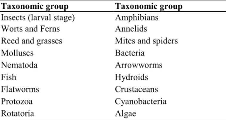
SSDs can be reconstructed using AVG and STDEV. For the 261 pesticide ingredients a total of 1143 AVG and STDEV values were calculated to be used as input for the toxic risk calculation per major taxonomic group ([AVGTax. Grp] and [STDEVTax. Grp]). A total of 18

different major taxonomical groups were recognized (Table 7) with up to 46 different species per group.

Table 7: Taxonomic groups represented in the toxicity data.

Taxonomic group Taxonomic group

Insects (larval stage) Amphibians

Worts and Ferns Annelids

Reed and grasses Mites and spiders

Molluscs Bacteria Nematoda Arrowworms Fish Hydroids Flatworms Crustaceans Protozoa Cyanobacteria Rotatoria Algae

4.1.1 Toxic risk per pesticide ingredient

From the calculated weekly exposure concentrations, the toxic risk for individual pesticide ingredients and major taxonomical groups can be calculated by the MS Excel function NORMDIST(x, mean, standard_dev, 1), that returns the normal cumulative distribution for the specified mean and standard deviation:

[PAFIngredient, Tax. Grp] = NORMDIST(10log([Present week’s final concentration (µg/l)]),

[AVGTax. Grp], [STDEVTax. Grp], 1)

The toxic risk per ingredient and per major taxon was subsequently averaged over the major taxonomic groups:

[PAFIngredient] = Avg([PAFIngredient, Tax. Grp])

The total permanent dataset to be generated by this calculation would be too large to be stored (122000 * 261 * 52 ≈ 1.7 giga-records). Therefore, the PAF values per ingredient and per gridcell are averaged over the 52 weeks. If all 261 pesticides would be present in all gridcells, this would produce a dataset of 32 mega-records. However, this is not the case. Only the non-zero values of the yearly average PAF in these records are retained for future use. For the same pesticide ingredients, the yearly average origin of loading percentages ([Old%], [Drift%], [Dry%], [Wet%] and [R&D%]) were also stored in this permanent database.

(27)

4.1.2 Overall toxic risk

The combined toxic risk of all 261 pesticide ingredients is evaluated by sequentially applying the following calculations (Traas et al., 2002):

1. For ingredients with the same Toxic Mode of Action (TMoA), concentration additivity is assumed. The weekly calculated concentrations per ingredient are transformed to Hazard Units per taxonomic group (HUIngredient, Tax. Grp), by dividing them by 10[AVGTax.Grp], followed

by summation (ΣHUTMoA, Tax. Grp). The weekly combined toxic risk per TMoA and per

major taxonomic group (msPAFTMoA, Tax. Grp) is then calculated by applying the MS Excel

function:

msPAFTMoA, Tax. Grp = NORMDIST(10log(ΣHUTMoA, Tax. Grp),0,Avg([STDEVTax. Grp]),1)

2. For ingredients with different TMoA, response addition per major taxonomic group is calculated, where it is assumed that the species are uncorrelated in their sensitivity for the different toxicants (Traas et al., 2002):

msPAFTax. Grp = 1- Π(1 - msPAFTMoA, Tax. Grp)

3. The final toxic risk (msPAF) is calculated as the average msPAFTax. Grp over taxonomical

groups, assuming equal weight of major taxonomical groups: msPAF = Avg(msPAFTax. Grp)

4. This final calculation would eventually contain about 6.5 mega-records (122000 * 52), which is too much too be stored permanently. Therefore, for all gridcells, the average [msPAF per 4 week period] is stored for future use (1.6 mega-records).

4.2 Handling temporary data, and subsequent gridcell

analyses

After this step in the calculation, the temporary database is emptied, and the next gridcell is selected. The entire calculation of exposure and risk starts a new loop:

End of the exposure and risk calculation process for a single gridcell Select next gridcell and GoTo Start (§3.2, page 19)

(28)

(29)

5. Method for validation of toxic risk

The risk scale (PAF) is dimensionless, but based on the sensitivity of species under lab conditions. In view of these facts, the association between risk and changes in biodiversity is not obvious. However, if the calculated overall toxic risk of pesticide exposure to aquatic species, that is expressed as the proportion of species expected to suffer effects from the exposure, is considerable and properly scaled, it is expected that this will be reflected in the species composition in the field.

Pesticide toxicity is not the only environmental condition governing species composition. A plethora of physico-chemical and habitat characteristics, as well as biological interactions all determine the type of community to be expected. The observed species composition in the field, in terms of the number and abundance of species, may directly be related to the predicted toxic risk of pesticide exposure. This will be easy to determine when the driving force of pesticide toxicity has a major influence over other driving forces. However, in view of the absence of extreme exposure levels, and the expected relevance of other driving forces, this approach was considered unlikely to yield sufficient explanatory power.

In order to be able to isolate the possibly slight effects of pesticide exposure from a dataset on measured biodiversity, as many as possible of the other driving forces have to be taken into account. Since the available dataset on biological and chemical observations in the field is only comprised of 212 sites, it is statistically impossible to include many of the variables possibly governing the waxe and wane of species. The number of predictors (related to degrees of freedom) should be at least a factor of about 10 less than the number of observations. Especially, with habitat characteristics that are generally expressed in categories the degrees of freedom will quickly exceed this requirement. It was therefore decided to limit the analysis to a few chemical water characteristics, next to pesticide toxic risk. The chemical characteristics used (pH, Chloride (Cl), Total P (TP), Kjeldahl N (KN) and DO) were selected based on an earlier analysis of the importance of factors determining aquatic community composition (Ertsen and Wortelboer, 2002). The influence of individual environmental predictors can only be discerned if the variables are not highly correlated. The dataset of chemical observations in field ditches, joined with the corresponding yearly

average of estimates on total toxic risk (msPAF) was therefore analyzed to reveal correlation structure. The association between the observed abundance of the macrofauna and

macrophyte species and the 6 abiotic predictors was established by Generalized Linear Model regression (GLM, McCullagh and Nelder, 1989), yielding a GLM model for every species. Assuming a Poisson distribution, species-specific regressions took the form:

(30)

2 2 1 2 2 1 2 2 1 2 2 1 2 2 1 2 2 1 msPAF m msPAF l DO k DO j KN i KN h TP g TP f Cl e Cl d pH c pH b a ) O ln( O i species of bundance A bserved O i, i, i, i, i, i, i, i, i, i, i, i, i A i A i ⋅ + ⋅ + + ⋅ + ⋅ + + ⋅ + ⋅ + + ⋅ + ⋅ + + ⋅ + ⋅ + + ⋅ + ⋅ + + = =

The 6 predictors were added stepwise to the model with linear and quadratic terms. The quadratic terms were introduced to address non-linear response relationships, such as optima. The stepwise procedure used the Bayesian Information Criterion (BIC, Schwarz, 1978) to restrict the addition of terms to those that have a significant contribution to the overall model (P < 0.05), making the full model highly significant. Calculations were conducted using S-Plus 2000, Professional Release 3 (MathSoft, Inc., Cambridge, MA, USA). The models are used to isolate the driving force of predicted pesticide toxicity on species assemblage.

(31)

6. Results and discussion

6.1 Toxic risk of individual pesticide ingredients

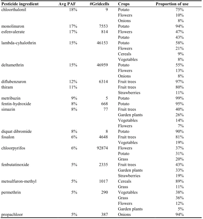
Only 46 out of the 261 pesticide ingredients used produced a non-zero risk in one or more of the nation-wide gridcells. This implies that for 215 out of 261 pesticide ingredients the physico-chemical behavior of the compounds, in combination with the sensitivity of aquatic species, produced no significant risk for these species in field ditches. The national average of the toxic risk for individual pesticide ingredients over gridcells (zero values excluded) is shown in Table 8 (Avg PAF). The number of gridcells where the pesticide is calculated to be responsible for a non-zero risk is counted (#Gridcells). The pesticide ingredients are linked to the crops they are applied on, as well as to the proportion of the pesticide applied to a

particular crop (Proportion of use). This table is further condensed by excluding

21 ingredients having an average risk below 5%, by grouping the 51 crops to 12 categories (see Table 9), and by excluding crop categories receiving less than 5% of a particular ingredient.

Table 8 makes it possible to score the crop categories on respective impact on pesticide toxic risk. Per crop category, the sum over pesticide ingredients is taken of the average PAF multiplied by the number of gridcells, multiplied by the proportion of use

(

å

(

[

] [

]

[

]

)

= × × = n Ingredient crop , i i i #Gridcells PropUse PAF Avg score Crop 1

). In Table 9, these sums are expressed relative to each other. The number of pesticide ingredients per crop category is also indicated.

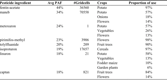
Table 8: Pesticide ingredients, arranged according to the average toxic risk they produce. Next to the number of gridcells where the ingredients produce non-zero risk, the associated crops and their proportion of pesticide use are also given.

Pesticide ingredient Avg PAF #Gridcells Crops Proportion of use

fentin-acetate 44% 36560 Potato 97% maneb 34% 70558 Potato 57% Onions 18% Flowers 14% metoxuron 24% 1 Potato 57% Vegetables 26% Flowers 13% pirimifos-methyl 23% 3906 Flowers 98%

tolylfluanide 20% 209 Fruit trees 90%

isoproturon 19% 17657 Cereals 97%

linuron 18% 21 Potato 58%

Vegetables 13%

Fodder maize 10%

Garden plants 6%

captan 18% 821 Fruit trees 84%

(32)

Pesticide ingredient Avg PAF #Gridcells Crops Proportion of use chloorthalonil 18% 9 Potato 75% Flowers 10% Onions 8% monolinuron 17% 7553 Potato 94% esfenvalerate 17% 814 Flowers 47% Potato 43% lambda-cyhalothrin 15% 46153 Potato 58% Flowers 21% Cereals 9% Vegetables 8% deltamethrin 15% 46959 Potato 55% Flowers 13% Onions 8%

diflubenzuron 12% 6314 Fruit trees 97%

thiram 11% Fruit trees 80%

Strawberries 11%

metribuzin 9% 5 Potato 99%

fentin-hydroxide 8% 668 Potato 95%

simazin 8% 77 Fruit trees 40%

Garden plants 26%

Vegetables 14%

Flowers 7%

diquat dibromide 8% 8 Potato 90%

fosalon 6% 4648 Fruit trees 81%

Vegetables 19%

chloorpyrifos 6% 92874 Flowers 37%

Potato 31%

Grass 20%

fenbutatinoxide 5% 2335 Fruit trees 43%

Garden plants 33% Strawberries 19% metsulfuron-methyl 5% 1017 Cereals 89% Grass 11% permethrin 5% 290 Vegetables 38% Grass 36% Flowers 12% Garden plants 5% propachloor 5% 387 Onions 94%

Table 9: Crops scored according to their impact on national risk.

Crop #Pesticides Score

Potato 27 58% Flowers 37 14% Cereals 20 9% Onions 23 8% Grass 17 4% Vegetables 35 3% Fruit trees 31 3% Sugar beet 22 1% Garden plants 34 0% Strawberries 19 0% Fodder maize 12 0% Maize 12 0%

(33)

On a nation-wide scale, it can be concluded that only 7 pesticide ingredients account for 95% of risk for the aquatic community. This is calculated by multiplying the Avg PAF of an ingredient with the number of gridcells where this ingredient is producing non-zero risk (Table 8). The resulting product of the individual components is expressed relative to each other. Also the use of the pesticides is specified. The top-7 pesticide ingredients are:

1. maneb (36%, fungicide)

2. fentin-acetate (24%, fungicide)

3. lambda-cyhalothrin (11%, pyrethroid insecticide)

4. deltamethrin (10%, pyrethroid insecticide)

5. chloorpyrifos (8%, insecticide)

6. isoproturon (5%, herbicide)

7. monolinuron (2%, herbicide)

With 58% of responsibility for aquatic risk (Table 9), the culture of potatoes contributes most prominently to toxic risk.

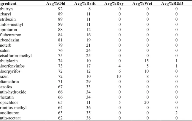
For the 46 pesticide ingredients, Table 10 gives the average percentage of the origin of pesticide loading in ditches. For most ingredients, the amount left over from past week’s exposure (Avg%Old) is the most prominent (58%). Drift exposure (Avg%Drift) is the second most important exposure pathway (33%), followed by the amount of pesticide in rain

(Avg%Wet, 5%). Dry deposition (Avg%Dry), as well as run-off and drainage (Avg%R&D) are negligible as pathways of exposure.

Table 10: Pesticide ingredients and their origin of aquatic exposure.

Ingredient Avg%Old Avg%Drift Avg%Dry Avg%Wet Avg%R&D

terbutryn 92 8 0 0 0 carbaryl 89 11 0 0 0 metribuzin 89 11 0 0 0 azinfos-methyl 89 11 0 0 0 isoproturon 88 12 0 0 0 diflubenzuron 84 16 0 0 0 carbendazim 81 19 0 0 0 dinoterb 79 21 0 0 0 fosalon 76 24 0 0 0 metsulfuron-methyl 75 25 0 0 0 terbutylazin 74 10 0 15 1 chloorfenvinfos 73 17 4 5 1 chloorpyrifos 72 12 6 10 0 atrazin 72 10 10 8 0 deltamethrin 71 29 0 0 0 triazofos 67 33 0 0 0 fentin-hydroxide 66 34 0 0 0 cyhexatin 66 34 0 0 0 propachloor 65 11 5 20 0 pirimifos-methyl 64 36 0 0 0 monolinuron 63 35 0 0 2 fentin-acetaat 62 38 0 0 0

(34)

Ingredient Avg%Old Avg%Drift Avg%Dry Avg%Wet Avg%R&D koperoxychloride 62 34 0 0 5 permethrin 61 39 0 0 0 DNOC 60 0 4 36 0 diazinon 59 23 0 19 0 lambda-cyhalothrin 57 43 0 0 0 simazin 55 41 0 0 4 linuron 53 47 0 0 0 fenbutatinoxide 51 49 0 0 0 mancozeb 50 50 0 0 0 maneb 49 39 0 0 13 dimethoaat 48 36 12 2 1 lindaan 46 5 12 37 0 MCPA 44 18 0 33 5 metoxuron 42 58 0 0 0 esfenvaleraat 42 58 0 0 0 zineb 42 58 0 0 0 chloorthalonil 41 49 1 8 0 thiram 41 59 0 0 0 diquat dibromide 39 52 0 0 9 heptenofos 39 61 0 0 0 tolylfluanide 36 64 0 0 0 mevinfos 34 51 14 1 0 methiocarb 30 63 0 7 0 captan 1 84 1 13 0 Total Average 58 33 1 5 1

6.2 Frequency distribution of total toxic risk (msPAF)

The frequency distribution of toxic risk for the aquatic ecosystem, associated with the agricultural use of pesticides is given in Figure 3.

0% 10% 20% 30% 40% 50% 60% 70% 80% 90% 100% 0 10 20 30 40 50 60

msPAF in percent of species affected

Cu mu lative frequ ency w ithi n a ll gri d cel ls an d 4-w eek p eri o d s

Figure 3 Frequency distribution of pesticide risk for all gridcells in the Netherlands and all 4-weeks periods in the year 1998.

(35)

Up to 75% of gridcells in place and time are expected to suffer minor impact with up to 5% of species affected. The maximum predicted impact of a mixture of a mixture of ingredients is estimated as 51%.

6.3 Mapping of total pesticide risk in field ditches

The 4-week average total toxic risk of pesticide use for the aquatic assemblage of species is depicted in the maps presented in Figure 4. From left to right, and from top to bottom, the maps represent the 13 periods of 4 weeks in 1998. White gridcells indicate a lack of data. The lightest pink color indicates an average toxic risk affecting less than 5% of the aquatic species potentially present in the field ditches. Increasingly, darker colors represent higher levels of expected effects.

The first three month of the year hardly any pesticides are used, and the toxic risk of the pesticide mixture stays below 5%. In April the pesticides start to be used. Overlaying the risk maps with the known distribution of crops, it can be identified that mainly the culture of flower bulbs, plant potatoes and fruit trees are responsible for this onset. The months of the year that suggest highest risk of pesticide use for aquatic species are June to August. The risks for the last three 4-week period are associated with the application of soil fumigation disinfectants, mainly in the flower bulb area.

(36)

Figure 4 Predicted ecotoxic risk (msPAFNOEC) of pesticide use in field ditches.

6.4 Effects of modeled risk: GLM-regression results

The abiotic set of field observations at 212 sites, that was used to explain the observed abundance of species, is having a correlation structure as presented in Table 11. The lower part of the table is giving the correlation coefficients (r), while the upper shaded part is related to the significance of the correlation. In the upper part, bold print is indicative for the

(37)

few significant relationships between the variables. Pesticide toxic risk (msPAF) only has a significant correlation with the chloride concentration (P<<0.001). As can be judged from examining Figure 5, this is due to only 4 outliers in the chloride data. It was decided not to correct for the chloride outliers in the abiotic dataset. The final objective of this study was only to relate the modeled risk of pesticide use to the species composition in the field. The analysis is specifically not meant to allow for a realistic prediction of community

composition in field ditches. Therefore, the observed significance in the correlation of the other predictor variables was considered of less importance, as was the omission of habitat characteristics that generally have a very important influence on species composition.

Table 11: Correlation structure (lower left) and significance of correlation (upper right) for the abiotic set of field observations.

CL TP KN MSPAF PH DO CL 0.564 0.284 0.000 0.000 1.000 TP 0.13 0.005 0.992 0.000 0.090 KN 0.16 0.25 0.874 0.363 0.007 MSPAF 0.40 -0.08 -0.11 1.000 0.069 PH 0.42 0.49 -0.15 0.04 0.000 DO -0.06 0.19 -0.24 -0.19 0.57

The scatterplot matrix in Figure 5 gives an idea about the value ranges of the variables in the abiotic dataset. Chloride (mg/l) 0 1 2 3 4 TotP (mgP/l) KjN (mgN/l) 0 10 20 30 40 msPAF (%) pH (unit) 0 1000 2000 3000 4000 5.0 10.0 15.0 0 4 8 12 4 6 8 O2 (mg/l)

Figure 5 Scatterplot matrix displaying the ranges, distributions of values and linear relationships in the abiotic dataset. The ellipse in the Cl-msPAF graph

(38)

Of the 344 macrofauna and 113 macrophyte species entered in the GLM regression, 306 and 92 species, respectively, did produce a regression formula with significant explanatory capacity for one or more of the 6 predictor variables. Figure 6 shows the frequency

distributions of the explained deviance of the regressions for macrofauna (average 35%) and macrophyte species (average 20%).

Macrofauna species (306) 0 10 20 30 40 50 60 70 10 20 30 40 50 60 70 80 90 100 Explained deviance % Fre que nc y .00% 10.00% 20.00% 30.00% 40.00% 50.00% 60.00% 70.00% 80.00% 90.00% 100.00% Cu mu la ti ve % Macrophyte species (92) 0 5 10 15 20 25 30 35 10 20 30 40 50 60 70 80 90 100 Explained deviance % Frequency .00% 10.00% 20.00% 30.00% 40.00% 50.00% 60.00% 70.00% 80.00% 90.00% 100.00% C u m u lativ e %

Figure 6 Frequency distributions of explained deviance in the GLM regression.

The regressions were also conducted without the addition of total toxic risk (msPAF) to the formulae. The average relative reduction in explained deviance by excluding msPAF was 16% and 10% (absolute: 6% and 2%), respectively for macrofauna and macrophytes. When the values of the abiotic predictors for each of the 212 sites are substituted into the calibrated regression formulae, the part of the linear predictor related to msPAF

(39)

( 2 i , 2 i , 1 msPAF m msPAF

l ⋅ + ⋅ ) is giving an indication of the “driving force” of toxic risk in terms of the abundance of the species. The msPAF part of the linear predictor is called “contribution of msPAF”. Negative values of the contribution indicate a force lowering the species’ abundance; positive terms increase the abundance. In Figure 7 the msPAF

contribution, irrespective of positive or negative contributions, is averaged over the

respective groups of species, and plotted against the local toxic risk (msPAF) for the aquatic community. -50 -40 -30 -20 -10 0 10 0 5 10 15 20 25 30 35 40

Toxic risk of all pesticides used (msPAF %)

m s PA F co ntr ibut ion to sp ecies co mp o sit io n Macrofauna species (306) Macrophyte species (92)

Figure 7 The relationship of mixture toxic risk and the modeled contribution of msPAF in terms of driving force to species abundance, separately for macrofauna and macrophytes.

Figure 7 illustrates that the macrophytes are relatively insensitive to the modeled pesticide toxic risk of pesticide mixtures. This is most probably due to the fact that only two

herbicides, comprising 7% of risk, are amongst the top-7 pesticides (see page 33). The

assembly of macrofauna species in the field is more strongly associated to mixture risk. Up to a toxic risk of about 10 percent, the toxicity is not reducing the abundance of species. When pesticide mixture risk is increasing, average modeled species abundance is gradually forced lower.

In terms of the predicted abundance of species (related to probability of occurrence), the negative trend of the msPAF-contribution with increasing toxic risk means that a sizeable abundance of species that may be predicted by the other predictors is gradually multiplied by an increasingly small number (minimum is: e-50≈ 10-22_{) at higher toxic risk. This implies that}

it becomes more and more likely that average species abundance, and thus probability of occurrence, is reduced at higher toxic risk of pesticide use.

(40)

6.5 Effects of modeled risk: Comparison with field data

A very weak relationship can be observed between predicted mixture risk values and the species composition in the field, both in terms of the number of species (Figure 8) and the overall abundance of individuals summed over species (Figure 9) in the macrofauna and macrophyte assemblages of species. To be able to observe these weak regression trends in the available biotic data, species with very high numbers at individual sites (>1400) and very scarcely occurring species (less than 10 individuals in the entire dataset) had to be removed from the analysis. The increased scatter introduced by those species totally obscured the weak signal present. After this treatment the dataset comprised 299 macrofauna and 106

macrophyte species. The high spread of the data can be caused by the fact that the data were gathered by about 35 different authorities, each operating their respective monitoring network with a non-standardized input of effort, skill and methodology. Although the slopes of the regression lines are clearly not significant (R2macrofauna,# species is 0.027 and R2macrofauna,total abundance is 0.01), the percentual difference between the predicted number of macrofauna

species at the calculated risks of 0% and 38% is 43%. For the number of macrofauna individuals, the percentual difference is 38%. Both reductions in species and individuals correspond remarkably well to the predicted risk of pesticide use for the aquatic community. Figure 10 gives the ranking distribution of the correlation coefficients between the pesticide toxic risk values (msPAF) and the observed abundance of individual species, separately for macrofauna and macrophytes. Over the 212 monitored sites, 29 percent of the macrofauna species (n=299) have a positive correlation between their abundance and toxic risk. These species may be marked “opportunists” since they most probably display indirect effects by filling the gap left by the 71% of “sensitive” species that are reduced in abundance with increasing toxic risk. For the macrophytes (n=106) the percentages of opportunist and sensitive species are 20 and 80 %, respectively. Figure 10 clearly illustrates why diversity indices are not very sensitive indicators for ecological effects over a wide range of toxic exposure. Very often, diversity effects are obscured by a shift in species composition. Some species are reduced and others are increased in their abundance, leaving the change in biodiversity indices neutral, while biodiversity itself changes considerably. Without the attribution of a tolerance score to the individual species or without relating the species

composition to a reference community, it is generally impossible to demonstrate toxic effects on diversity, unless an extremely high toxicity is detrimental to the majority of species. Table 12 gives the top-10 listing of both sensitive and opportunist species in macrofauna and macrophytes, respectively. At the moment, there is not sufficient knowledge available to compare the listing in table 12 to a known sensitivity of the individual species.

(41)

0 10 20 30 40 50 60 0 5 10 15 20 25 30 35 40

Num b er of M acro fau na sp eci es ob serve d 0 1 2 3 4 5 6 7 8 9 Num b er of M acro fy te sp eci es ob serve d

Macrofauna number of species Macrophyte number of species

Linear regression macrophytes: y = 0.0061x + 1.3817 Linear regression macrofauna: y = -0.1472x + 12.942

Figure 8 The relationship of the observed number of species and toxic risk for macrofauna and macrophyte species.

0 500 1000 1500 2000 2500 3000 3500 4000 0 5 10 15 20 25 30 35 40

Over al l abu n d an ce o f M a cro fau n a s p ec ie s ob ser ved 0 50 100 150 200 250 Over al l abu n d an ce o f M a cro fyt e s p ec ie s ob ser ved

Macrofauna overall abundance Macrophyte overall abundance

Linear regression macrophytes: y = 0.2229x + 36.339 Linear regression macrofauna: y = -3.8481x + 389.35

Figure 9 The relationship of the observed number individuals and toxic risk for macrofauna and macrophyte species.

(42)

-0.4 -0.3 -0.2 -0.1 0 0.1 0.2 0.3 0.4 0% 10% 20% 30% 40% 50% 60% 70% 80% 90% 100% Percent of species Co rr el at io n c o ef fi c ien t o f msP A F vs s p e ci es abund an ce Correlation macrofauna Correlation macrophytes Opportunists Sensitives

Figure 10 Distribution of the signed correlation coefficient (r2) between pesticide toxic risk (msPAF) and the observed abundance of individual macrofauna (n=299) and macrophyte (n=106) species.

Table 12: The top-10 in sensitive and opportunist macrofauna and macrophyte species.

Macrofauna Macrophytes

Sensitives Opportunists Sensitives Opportunists

Helochares Anisus leucostomus Butomus umbellatus Phragmites australis Limnesia maculata Radix gr peregra Solanum dulcamara Spirodela polyrhiza Radix ovata Haliplus lineatocollis Nuphar lutea Callitriche

Erpobdella octoculata Tetanocera sp Peucedanum palustre Lemnacea

Piona imminuta Chironomus gr plumosus Nymphaea alba Potamogeton pusillus Polypedilum

nubeculosum

Polypedilum gr nubeculosum

Galium palustre Potamogeton pectinatus Collembola Valvata cristata Mentha aquatica Glechoma hederacea Piona conglobata Neomysis integer Ranunculus sceleratus Juncus effusus

Mideopsis orbicularis Physa acuta Rumex hydrolapathum Ceratophyllum demersum Arrenurus crassicaudatus Cricotopus gr sylvestris Lycopus europaeus Wolffia arrhiza

The present validation study only gives an indication that the effects on aquatic ecosystems, predicted from the crop-based use of pesticides, may indeed be realistic. However, the

available data on species abundance for the year 1998, obtained from the monitoring network of the Water Boards, proved to be too low in coverage (only 212 sites) to be quantitatively conclusive.

(43)

References

De Vries, F and J Denneboom. 1992. De bodemkaart van Nederland digitaal. Wageningen, DLO-Staring Centrum.

De Zwart, D. 2002. Observed regularities in SSDs for aquatic species. In: Posthuma, L, TP Traas and GW Suter. Species Sensitivity Distributions in Ecotoxicology. Lewis Publishers, Boca Raton, FL, USA.

Ertsen, ACD and FG Wortelboer. 2002. Ristori 2001; Responsmodellen voor aquatische systemen. Royal Haskoning report 38931/R0325/DE/DenB.

Leistra M, AMA van der Linden, JJTI Boesten, A Tiktak and F van den Berg. 2000. PEARL: a model for pesticide behaviour and emissions in soil-plant systems. RIVM Rapport 711401009; Alterra report 28. 107 p in English.

McCullagh, P and JA Nelder. 1989. Generalized Linear Models, 2nd edition. Chapman and Hall, London.

Meinardi, CR and CGJ Schotten. Stromen van water en stikstof vanaf en door de bodem naar het open water. RIVM report in preparation.

Posthuma, L., TP Traas and GW Suter. 2002. Species Sensitivity Distributions in Ecotoxicology. Lewis Publishers, Boca Raton, FL, USA.

Schwarz, G. 1978. Estimating the Dimension of a Model. The Annals of Statistics, 6, pp. 461-464.

TNO. 2002. Atmosferische depositie van pesticiden, PAK en PCB’s in Nederland. TNO report R 2002/606. 107 p in Dutch.

Traas, TP, D van de Meent, L Posthuma, T Hamers, BJ Kater, D de Zwart and T Aldenberg. 2002. The potentially affected fraction as a measure of ecological risk. In: Posthuma, L, TP Traas and GW Suter. Species Sensitivity Distributions in Ecotoxicology. Lewis Publishers, Boca Raton, FL, USA.

(44)

(45)

Appendix 1: Pesticides and physico-chemical properties

Active pesticide ingredients with estimates of physico-chemical properties (TMoA = toxic mode of action; kW = degradation rate constant in water; Kom = artitioning coefficient between water and soil organic matter; kS = degradation rate constant in soil; VdW = vertical displacement velocity to water; VdS = vertical displacement velocity to soil). The table is sorted according to toxic mode of action.

Toxicity data are omitted because the dataset comprises nearly 1150 records.

Active ingredient TMoA kW

(1/wk) Kom (1/wk)kS (cm/s)VdW (cm/s)VdS triazamaat Unknown 1.00 138.95 0.50 Na-p-tolueensulfonchloramide Unknown 1.00 7.20 0.50 ethefon Unknown 1.00 138949.55 0.43 benazolin(-ethyl) Unknown 1.00 56.60 0.50 triforine Unknown 1.00 5568.19 0.23 buminafos Unknown 1.00 138.95 0.50 dazomet Unknown 1.00 7.20 0.69 polyvinylacetaat Unknown 1.00 3.27 0.50 trinexapac-ethyl Unknown 1.00 3.40 0.50 pyridaben Unknown 1.00 233034.38 0.50 d-karvon Unknown 1.00 138.95 0.50 azijnzuur acid 1.00 0.72 0.50 boraat acid 1.00 0.14 0.50 formaldehyde aldehyde 2.31 1.97 0.50 glutaaraldehyde aldehyde 1.00 0.71 0.50 metaldehyde aldehyde 1.00 109.65 0.49

cymoxanil aliphatic nitrogen 1.00 3738.89 0.50 dodine aliphatic nitrogen 3.47 0.18 0.24 guazatine aliphatic nitrogen 1.00 138.95 0.50

propyzamide amide 0.09 93.63 0.08 diflufenican anilide 1.00 13453.65 0.02 abamectine antibiotic 1.00 1483.98 0.17 kasugamycine antibiotic 1.00 5.35 2.91 streptomycine-sulfaat antibiotic 1.00 7.20 0.50 validamycine antibiotic 1.00 0.00 0.50 chloorfacinon anticoagulant 1.00 43090.63 0.50 fentin-acetaat antifeedants 1.00 776.71 0.50 fentin-hydroxide antifeedants 1.00 5459.37 0.06 chloorthalonil aromatic 0.69 491.39 0.16 0.12 0.00 dichloran aromatic 1.00 93.73 0.50 kresol aromatic 1.00 138.95 0.50 nitrothal-isopropyl aromatic 1.00 603.57 0.50 clodinafop-propargyl aryloxyphenoxypropionic 4.62 138.95 6.07 fenoxaprop-P-ethyl aryloxyphenoxypropionic 1.00 2578.86 0.54 fluazifop-P-butyl aryloxyphenoxypropionic 1.00 138.95 0.50 haloxyfop-ethoxyethyl aryloxyphenoxypropionic 1.00 4452.20 0.50 haloxyfop-P-methyl aryloxyphenoxypropionic 1.00 2688.47 0.09 propaquizafop aryloxyphenoxypropionic 1.00 7517.42 0.50 quizalofop-ethyl aryloxyphenoxypropionic 1.00 138.95 0.50 quizalofop-P-ethyl aryloxyphenoxypropionic 1.00 138.95 0.50 1-naftylaceetamide auxins 1.00 28.15 0.50 1-naftylazijnzuur auxins 1.00 77.20 0.50 3-indolylazijnzuur auxins 1.00 15.43 0.50 3-indolylboterzuur auxins 1.00 86.73 0.50 flutolanil benzanilide 1.00 8283.18 0.02 carbendazim benzimidazole 0.17 103.34 0.05 thiabendazool benzimidazole 1.00 598.61 0.01 thiofanaat-methyl benzimidazole 1.00 622.71 0.50

ethofumesaat benzofuranyl alkylsulfonate 1.00 147.43 0.16 0.43 0.15 benfuracarb benzofuranyl methylcarbamate 0.69 4200.46 0.50

Ecological effects of pesticide use in the Netherlands: Modeled and observed effects in the field ditch

Abstract

Contents

Samenvatting

Summary

1.

Introduction

1.1

Problem definition

1.2

Towards quantification of risks

1.3

Aims

2.

Available data

2.1

Data on active pesticide ingredients

2.2

Grid-based soil properties

2.3

Climatic data

2.4

Land use and Crops

2.5

Application regimen of pesticide ingredients per crop

2.6

Direct spray drift of pesticide ingredients to a field ditch

2.7

Direct transfer of pesticide ingredients to the soil

2.8

Pesticide ingredients in air and wet precipitation

2.9

Pesticide concentration in run-off and drainage water

2.10

Chemical and species monitoring data in ditches

3.

Methods for calculating exposure

3.1

Exposure assumptions and data storage

3.2

Start of the exposure and risk calculation process for a

single gridcell

3.2.1 Amount of precipitation transferred to ditch and soil

3.2.2 Concentration of pesticide ingredients in rain water

3.2.3 Aquatic exposure by direct spray drift

3.2.4 Aquatic exposure by dry deposition

3.2.5 Soil loading by application of pesticides, A

3.2.6 Soil loading by dry deposition of pesticide ingredients, B

3.2.7 Soil loading of pesticide ingredients by rain input, C

3.2.8 Total loading of soil

3.2.9 Concentration in run-off and drainage water

3.2.10 Amount of R&D water transferred to ditch

3.2.11 Iteration of the weekly concentration in ditch water

3.3

Gridcell-based concentration results

4.

Methods for calculating toxic risk for aquatic

species

4.1

The method of toxic risk calculation

4.1.1 Toxic risk per pesticide ingredient

4.1.2 Overall toxic risk

4.2

Handling temporary data, and subsequent gridcell

analyses

5.

Method for validation of toxic risk

6.

Results and discussion

6.1

Toxic risk of individual pesticide ingredients

å

(

[

] [

]

[

]

)

6.2