Ductile fracture modelling of Single Edge Notched Tension (SENT) tests using the complete Gurson damage model

(1)

damage model

Tension (SENT) tests using the complete Gurson

Ductile fracture modelling of Single Edge Notched

Academic year 2019-2020

Master of Science in Electromechanical Engineering

Master's dissertation submitted in order to obtain the academic degree of

Counsellor: Vitor Soares Rabelo Adriano

Supervisors: Prof. dr. ir. Stijn Hertelé, Prof. dr. ir. Wim De Waele

Student number: 01500240

(2)

(3)

damage model

Tension (SENT) tests using the complete Gurson

Ductile fracture modelling of Single Edge Notched

Master of Science in Electromechanical Engineering

Master's dissertation submitted in order to obtain the academic degree of

Counsellor: Vitor Soares Rabelo Adriano

Supervisors: Prof. dr. ir. Stijn Hertelé, Prof. dr. ir. Wim De Waele

Student number: 01500240

(4)

Preface

This thesis marks the end of my final year as a student. A lot of hard work and many hours went into its making. The result would not have been possible without the help and pleasant company, even through video calls, of many people, who I would like to thank here.

First of all, I would like to thank my supervisors prof. dr. ir. Stijn Hertelé and prof. dr. ir. Wim De Waele. They provided a lot of helpful and critical remarks, and we had many insightful discussions.

Next, I would like to especially thank my counsellor ir. Vitor Adriano for his amazing support in this entire project. He was always ready to help me with any problems. Especially his help and ingenious ideas during the experiments were invaluable.

I also want to thank ir. Robin Depraetere, ir. Rahul Kumar and dr. ir. Wouter Ost for their assistance in setting up the experiments, and ir. Marcus Silvestre and dr. ir. Kaveh Samadian for their help in the post-processing of the DIC results.

Additionally, I want to thank Johan Van Den Bossche and the technical staff of Labo Soete for the machining of the test specimens.

Finally, my thanks go to my girlfriend Veronique Moons, my friends and my family for supporting me during the creation of this thesis and during all previous years.

Ben Van Raemdonck

The author gives permission to make this master dissertation available for consultation and to copy parts of this master dissertation for personal use. In all cases of other use, the copyright terms have to be respected, in particular with regard to the obligation to state explicitly the source when quoting results from this master dissertation.

(5)

Ductile fracture modelling of Single Edge

Notched Tension (SENT) tests using the

complete Gurson damage model

Ben Van Raemdonck

Supervisors: Prof. dr. ir. Stijn Hertelé, Prof. dr. ir. Wim De Waele Counsellor: ir. Vitor Soares Rabelo Adriano

Master’s dissertation submitted in order to obtain the academic degree of Master of Science in Electromechanical Engineering

Abstract

To determine if a structure containing defects needs to be repaired, an engineering critical assess-ment (ECA) needs to be made. For a high level ECA, the toughness is measured by laboratory tests, such as the single edge notched tension (SENT) test, in the form of a tearing resistance curve. The standards which describe these tests contain many validity criteria, but there are no criteria dealing with the presence of volumetric flaws in the test specimens. Nevertheless, it was shown experimentally that volumetric flaws have a large influence on the resulting resistance curves of SENT tests in a previous research project.

This thesis aims to replicate the results of the SENT tests with drilled holes through numerical finite elements (FE) modelling. The complete Gurson damage model (CGM) is implemented in the FE model, to enable crack growth and weakening of the material to be simulated. A cali-bration procedure using tensile tests of notched round bars and a surrogate based optimisation method was developed and executed to obtain the parameters of the CGM. Subsequently, this damage model was employed to model SENT tests.

The calibration procedure did not yield a unique set of parameter values. Nevertheless, a parameter set with a good correspondence with the results of the performed experiments was found. The SENT model underestimated the tearing resistance obtained in the SENT test without holes. The tearing resistance curves of the specimens containing drilled holes were able to be simulated with a certain accuracy. Furthermore, the results of the SENT models showed that the tearing resistance is reduced by holes with greater cross sectional area or a greater depth.

(6)

Ductile fracture modelling of Single Edge Notched

Tension (SENT) tests using the complete Gurson

damage model

Ben Van Raemdonck

Supervisors: Prof. dr. ir. Stijn Hertelé and Prof. dr. ir. Wim De Waele Councellor: ir. Vitor Soares Rabelo Adriano

Abstract— To determine if a structure containing defects needs to be repaired, an engineering critical assessment (ECA) needs to be made. For a high level ECA, the tough-ness is measured by laboratory tests, such as the single edge notched tension (SENT) test, in the form of a tearing re-sistance curve. Previous research has shown experimentally that the results of these tests are influenced by the pres-ence of volumetric flaws in the test specimens. This thesis aims to replicate the results of SENT tests with drilled holes through numerical finite elements (FE) modelling, using the complete Gurson damage model (CGM). To this end, a cali-bration procedure to determine the parameters of the CGM was developed and performed.

Keywords— SENT, complete Gurson model (CGM), FEA

I. introduction

One of factors that determine the integrity of a structure is the fracture toughness in the presence of flaws, such as porosities or cracks. Non-destructive testing is commonly used at critical positions like welds to find such flaws. Sim-ple workmanship rules exist to accept flaws, using a high level of conservatism. If a flaw is rejected by these work-manship rules, it is deemed a defect and must be either repaired or further analysed by an engineering critical as-sessment (ECA). Fracture mechanics theory is applied in an ECA to determine if leaving the unaltered defect is safe. For a high level ECA, the toughness is measured by labo-ratory tests in the form of a tearing resistance curve, which displays the required applied crack driving force to achieve a certain crack growth. One form of such a laboratory test is the single edge notched tension (SENT) test, where a gradually increasing displacement is applied to a pre-cracked test specimen. The standards which describe the tests to obtain a tearing resistance curve contain many va-lidity criteria, but there are no criteria dealing with the presence of volumetric flaws in the test specimens. Never-theless, it was shown experimentally that volumetric flaws have a large influence on the resulting resistance curves of SENT tests in a previous research project [1].

This thesis aims to replicate the results of the SENT tests with drilled holes through numerical finite elements (FE) modelling. A damage model is required in the FE model, to enable crack growth and weakening of the ma-terial to be simulated. Thus, the goal of this thesis is to develop and execute a calibration procedure to obtain the parameters of a suitable damage model, and subsequently

use this damage model to model SENT tests. II. Complete Gurson damage model

The complete Gurson model (CGM) is a micromechanics-based model to describe ductile failure. It is an adjustment of the original Gurson model, where a modification of the von Mises yield surface is proposed by introducing the hy-drostatic stress and a new parameter called the void volume fraction (f ). The yield surface of the CGM is defined as:

( σe σf )2 + 2q1f∗cosh ( 3q2σm 2σf ) − 1 − q2 1f∗2= 0 (1)

where σeis the equivalent von Mises stress, σm is the

hy-drostatic stress, σf is the flow stress, f∗ is the modified

void volume fraction and q1 and q2are material constants.

The void volume fraction is modified to artificially increase after void coalescence has begun as follows:

f∗(f ) =          f if f < fc fc+ f_u∗− fc fF− fc (f− fc) if fc ≤f ≤ fF fu∗ if fF <f (2)

where fc is the critical void volume fraction at which

coa-lescence starts, fFis the final void volume fraction at which

failure occurs and f_u∗ is the ultimate value of the modified void volume fraction which is taken as 1/q1. Thomason’s

plastic limit load criterion is incorporated in the CGM to predict the start of void coalescence during simulations, which can be different for each integration point. The void volume fraction starts at the initial void volume fraction (f0) and its evolution can be split into two contributions:

void nucleation and the growth of existing voids. Void nu-cleation is assumed to be strain-controlled and described as: ˙ fnucleation= fN SN √ 2πexp [ −1 2 ( ϵpeq− ϵN SN )2] ˙ϵp_eq (3) where fN is the volume fraction of void nucleating particles,

ϵN is the mean void nucleation strain, SN is corresponding

standard deviation and ϵp

eq is the equivalent plastic strain.

The void growth is described using conservation of mass as:

˙

fgrowth= (1− f)˙ϵ p

(7)

where ˙ϵp_ii is the plastic hydrostatic strain.

Thus, seven parameters (q1, q2, f0, fF, fN, ϵN, SN) need

to be identified in order to use the CGM, alongside the damage-free true stress-strain curve of the material.

III. Experiments

The test specimens were machined out of steel grade L480 extracted from a pipe. Experiments using smooth round bars were performed to determine the damage-free true stress-strain curve of the material. Experiments using notched round bars with a minimum cross sectional radius of 3 mm and notch radii in the longitudinal direction (r) of 1.2 mm, 2 mm and 6 mm were performed to induce dif-ferent stress states. The stress triaxiality induced by these notch radii is similar to the stress triaxiality present at the crack tip during a SENT test (1−1.7). The test setup con-sists of an extensometer measuring the elongation, a load cell measuring the applied force, a digital image correlation (DIC) system measuring the displacement field, and a dig-ital single-lens reflex (DSLR) camera used to measure the diameter reduction.

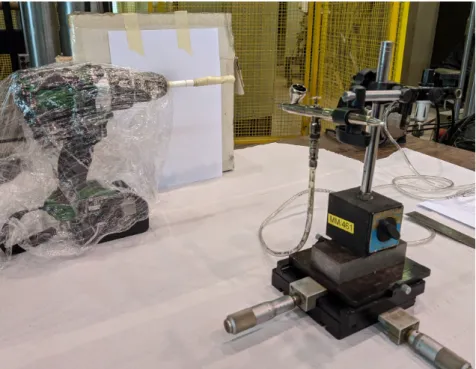
In order to use DIC, a black speckle pattern needs to be applied to the surface of the specimen after it has been painted white. Since the specimens, and hence the field of view, are small, the required speckle size (3 - 5 pixels) is very fine. With the camera settings used, an average speckle diameter of 45.4 µm is required, for which no con-ventional methods are available. Therefore, a novel method was developed, where an airbrush is used to spray acrylic paint onto the specimen (Fig. 1). By continuously evalu-ating the applied speckle quality through images taken by the DIC system, the method was optimised. It was found that through a mixture of 1/3 paint and 2/3 water, a noz-zle opening of 1/4 of the maximum opening and a distance between the nozzle and the specimen of 21 cm a high qual-ity speckle pattern can be applied. The speckle pattern is applied homogeneously to the specimen surface by rotating the specimen with a drill, and linearly moving the airbrush calibre by a moveable magnetic platform.

Fig. 1. Setup to apply the speckle pattern

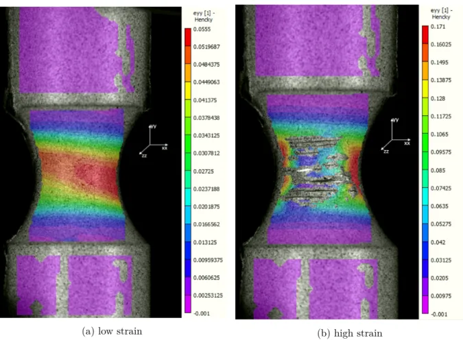
However, the applied paint, and thus speckle pattern required for the analysis, peels off at high deformations (Fig. 2). Hence, the strains and deformations are not able to be determined for high deformation levels inside the

notch. Since the goal is to use the experimental results to calibrate the complete Gurson damage model, the re-sults at high deformations would be the most relevant, as here the accumulated damage will have a large influence on the results. For this reason, the DIC results will not be used in the calibration procedure. Instead, the DIC re-sults were used to determine the diameter reduction of the specimen in the direction orthogonal to the diameter re-duction measured by the DSLR camera, in order to check for anisotropy. Only a minor degree of anisotropy was ob-served.

Fig. 2. Paint peeling of at high deformations (specimen with r = 6 mm)

The subsequent images taken by the DSLR camera dur-ing the test are analysed through a Python script, which generates a gateway to image processing software ImageJ2 [2, 3]. The edges of the specimen are found in each im-age through a colour threshold, creating a binary imim-age (Fig. 3). Subsequently, all images are analysed in order to find the minimal distance between the edges of the speci-men to find the minimal diameter, and thus the diameter reduction in comparison to the initial image. In the first image, the median distance in pixels between the edges of the specimen outside the notch is used to determine the conversion factor between pixels and mm.

(8)

IV. Complete Gurson model (CGM) calibration The CGM contains seven parameters (q1, q2, f0, fF,

fN, ϵN, SN) which need to be calibrated, alongside the

damage-free true stress-strain curve of the material. This damage-free stress-strain curve before necking was deter-mined from the uniaxial tensile test data of the smooth round bar specimen. After necking, the true stress-strain curve is approximated by:

σ = σu [ w(1 + ϵ− ϵu) + (1− w) ( ϵϵu ϵϵu u )] (5) where σ is the true stress, ϵ is the true strain, σuis the true

stress at the onset of necking, ϵu is the corresponding true

strain and w is a weight factor. This weight factor was de-termined to be 0.5 by comparing simulated force-elongation curves with the corresponding experimental curve, without using a damage model (Fig. 4). This procedure is possible because the void volume fraction does not have a signifi-cant effect on the tensile properties until just before final fracture for this geometry.

Fig. 4. The simulated and experimental results of the smooth round bar, for different values of w

The parameters q1and q2were determined based on the

calibration by Faleskog et al. [4]. They are tabulated as function of the strength (σ0/E) and Hollomon strain

hard-ening exponent N of the material, determined to be 0.0023 and 0.1412 respectively. The resulting parameter values are q1= 1.62 and q2= 0.875. The parameters ϵN and SN

were adopted from literature to be 0.3 and 0.1 respectively. The parameters f0, fN and fFwere determined by

surro-gate based optimisation. The working principle is schemat-ically shown in Fig. 5

In the design of experiments step, a uniform distri-bution of parameter sets was selected by the method ’Latin hypercube sampling with multidimensional unifor-mity’ (LHSMDU) [6]. In the next step, numerical simu-lations with these parameter sets were performed in the FE software ABAQUS© (version 2019), using a user sub-routine implementing the CGM [7]. A nominal mesh size of 0.3 mm x 0.3 mm x 0.3 mm was used in region where the CGM was applied. It should be noted that the CGM is mesh dependant. The surrogate model was constructed

Fig. 5. Surrogate based optimisation working principle [5]

as an objective function comparing the experimental and numerical force-elongation and force-diameter reduction curves as follows:

OBJ = ∑

r=1.2, 2, 6 mm

(SSel+ SSdiam)r (6)

where OBJ is the objective function value, SSelis the sum

of squares between the force-elongation curves and SSdiam

is the sum of squares between the force-diameter reduction curves. This objective function was modelled as a second order polynomial with variables f0, fN and fF, and ten

unknown coeﬀicients. These coeﬀicients were found by de-termining the value of the objective function through ten simulations with the parameter sets chosen by LHSMDU, and solving the resulting system of equations. Finally, the optimal parameter sets are equal to the roots of the polyno-mial. Two surfaces of optimal parameter sets were found. Simulations were performed with three sets, and a good agreement with the experimental curves was found for all three. Nevertheless, there were significant differences be-tween these sets, so a iterative surrogate based method to find a unique optimum was proposed. One set was selected (f0= 0.0020, fN = 0.0139, fF = 0.2364), which has a good

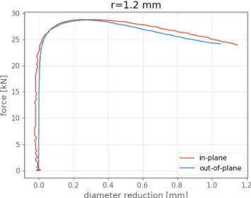
agreement with the final unstable fracture of the specimens with notch radii 1.2 mm (Fig. 6) and 2 mm, while the duc-tility is underestimated for r = 6 mm.

Fig. 6. The results of the experiment and simulation with calibrated parameters, for the specimen with r = 1.2 mm

(9)

V. Single edge notched tension (SENT) models The results of the numerical SENT model, implement-ing the calibrated CGM, are compared with the SENT tests performed previously. In the experiments, the crack growth (∆a) was determined by direct current potential drop (DCPD) and unloading compliance (UC) methods. In the numerical models, The CTOD was determined through the distance between two nodes at the crack mouth and two nodes 1 mm below the surface, according to the procedure outlined in BS8571 [8] for clamped specimens. The crack growth due to blunting was approximated as CTOD/2 be-fore tearing initiates. The average crack growth due to tearing was found by dividing the projected area of the el-ements where final failure has occurred (f > fF) by the

width of the specimen. The same mesh size as during the calibration was used, as the CGM is mesh dependant.

First, the resistance curves of the reference specimen without holes (A12B2) are compared (Fig. 7). The agree-ment is good for the first half of the crack growth (∆a < 1.25). However, when a large amount of crack growth has occurred, the crack growth for a given crack driving force is overestimated by the numerical results. The fracture initia-tion toughness, defined by the intersecinitia-tion of the tearing re-sistance curve with a line defined by CT OD = 2(∆a− 0.2) (Fig. 7), is underestimated by the simulation.

Fig. 7. Comparison of the experimental and numerical resistance curves of the SENT specimen without holes, where the fracture initiation toughness is indicated

The drilled holes in the experiments had a circular cross section with an area of 0.79 mm2 _{and a nominal depth of}

9 mm. These are approximated by three types of holes: the first type of hole has a square cross section with an area of 0.81 mm2 _{Using the second type, each hole has a more}

rounded cross section, but with a larger area of 1.08 mm2_.

Finally, a rounded hole with a depth of 9.3 mm was used to evaluate the influence of the depth. The different types of holes are compared in Fig. 8. It can be seen that a greater cross sectional area of the holes causes a significant reduction in tearing resistance, and an increased depth a less significant reduction.

The numerical simulations indicated the same trend ob-served in the experimental results; the tearing resistance is decreased by drilled holes, and decreased more severely by

Fig. 8. Comparison of the resistance curves using different types of holes

holes in a straight line (A12B3) than holes in a zig-zag pat-tern (A12B5) (Fig. 9). The decrease in tearing resistance is accurate up to a crack growth of 1 mm, but underesti-mated thereafter. A relatively good agreement with the experimental fracture initiation toughness was found for the specimens modelled with square holes.

Fig. 9. Comparison of the experimental and numerical resistance curves

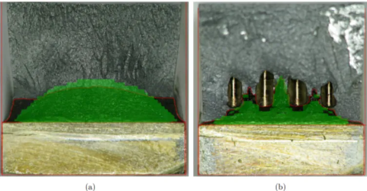
Additionally, the crack growth was compared by over-laying the modelled crack, at the same force as the applied force when the specimen failed, on the fracture surface of the SENT specimens (Fig. 10). For the smooth specimen, the crack growth was slightly overestimated in the mid-dle of the specimen, and severely underestimated at the edges. This underestimation can be explained, as here fail-ure occurred by shearing, evidenced by shear lips, and the CGM is not capable of predicting void growth due to shear-ing. For the specimens with holes, the shape of the crack growth at final failure was able to be accurately modelled. The modelled average crack growth at final fracture cor-responded well with the experiments for specimens A12B2 and A12B3, but was overestimated for specimen A12B5.

(10)

Fig. 10. Overlay of the modelled crack on the fracture surface, where (a): A12B2 and (b):A12B3 square holes

VI. Acknowledgements

The author would like to acknowledge the support of his supervisors Prof dr. ir. Stijn Hertelé and Prof dr. ir. Wim De Waele and the help of his counsellor ir. Vitor Soares Rabelo Adriano.

References

[1] E. Cardon, “Experimental deformation and fracture analysis of sharp notched welds containing volumetric flaws,” 2019.

[2] C. T. Rueden, J. Schindelin, M. C. Hiner, B. E. De-Zonia, A. E. Walter, E. T. Arena, and K. W. Eliceiri, “Imagej2: Imagej for the next generation of scientific image data,” BMC bioinformatics, vol. 18, no. 1, p. 529, 2017.

[3] J. Schindelin, I. Arganda-Carreras, E. Frise, V. Kaynig, M. Longair, T. Pietzsch, S. Preibisch, C. Rueden, S. Saalfeld, B. Schmid, et al., “Fiji: an open-source platform for biological-image analysis,” Nature meth-ods, vol. 9, no. 7, pp. 676–682, 2012.

[4] J. Faleskog, X. Gao, and C. Fong Shih, “Cell model for nonlinear fracture analysis - I. Micromechanics calibra-tion,” International Journal of Fracture, vol. 89, no. 4, pp. 355–373, 1998.

[5] N. V. Queipo, R. T. Haftka, W. Shyy, T. Goel, R. Vaidyanathan, and P. Kevin Tucker, “Surrogate-based analysis and optimization,” 2005.

[6] J. L. Deutsch and C. V. Deutsch, “Latin hypercube sampling with multidimensional uniformity,” Journal of Statistical Planning and Inference, vol. 142, pp. 763– 772, mar 2012.

[7] Z. L. Zhang, C. Thaulow, and J. Ødegård, “Complete Gurson model approach for ductile fracture,” Engineer-ing Fracture Mechanics, vol. 67, no. 2, pp. 155–168, 2000.

[8] BS 8571:2018, “Method of test for determination of fracture toughness in metallic materials using single edge notched tension (sent) specimens,” standard, The British Standards Institution, 2018.

(11)

List of Figures

1.1 The influence of drilled holes on tearing resistance, with holes not present in

A12B2, and holes present in A12B3 and A12B5 [1] . . . 2

2.1 Initial values of stress triaxiality and lode angle [4] . . . 7

2.2 Three stages of ductile fracture [5] . . . 8

2.3 Influence of stress triaxiality on the equivalent plastic strain at failure in the middle of the specimen. Figure (a) shows a medium strength steel and figure (b) shows a high strength steel [14] . . . 9

2.4 Stress triaxiality evolution during loading for different notch radii, with a/r = 0.2, 0.6, 1.2, 2.0, 3.0 [14] . . . . 9

2.5 3D fracture locus showing the effect of stress triaxiality (η) and Lode angle (¯θ) on the equivalent plastic strain at failure ( ¯ϵf) [4] . . . 10

2.6 A crack growth resistance curve [19] . . . 11

2.7 Possible specimen geometries for fracture toughness tests . . . 12

4.1 Geometry of the smooth specimen (dimensions in mm) . . . 21

4.2 Geometry of the notched round bar specimens (dimensions in mm) . . . 21

4.3 Influence of r and n on stress triaxiality evolution . . . . 22

4.4 Experimental test setup . . . 24

4.5 Correlation of subsets of the speckle pattern [38] . . . 25

4.6 Setup to apply the speckle pattern . . . 27

4.7 Example of the applied speckle pattern (inside the notch of the specimen with r = 2 mm) . . . . 28

4.8 Example DSLR camera pictures . . . 29 iv

(15)

LIST OF FIGURES v

4.9 Paint peeling off the specimen when the whole specimen surface is painted . . . . 29

4.10 Image processed by ImageJ2 to find the edges of the specimen . . . 30

4.11 Results of the force, elongation and diameter reduction . . . 31

4.12 Example axial strain fields from DIC analysis, with paint peeling off at high strain (specimen with r = 6 mm) . . . . 33

4.13 Setup used to determine the anisotropy . . . 34

4.14 Comparison of the diameter reduction to determine the anisotropy . . . 34

5.1 Surrogate based optimisation working principle [46] . . . 37

5.2 An example of LHS with N_s = 6 and two dimensions [46] . . . 39

5.3 Comparison of sampling sets generated by MCS, LHS and LHSMDU [48] . . . . 39

5.4 The negligible influence of damage on the tensile behaviour of smooth round bars [50] . . . 41

5.5 The simulated and experimental results of the smooth round bar, for different values of w . . . . 42

5.6 The Ramberg-Osgood and Hollomon material model curve fit, compared with the used post-necking extrapolation . . . 43

5.7 Influence of the mesh size on a resistance curve [26] . . . 44

5.8 Mesh in the region around the notch where the CGM is applied (r = 1.2 mm) . . 45

5.9 Illustration of boundary conditions and nodes used in post-processing of the spec-imen with r = 2 mm . . . . 45

5.10 Example of a spline used to interpolate the data points . . . 46

5.11 Splines of the results of the experiments and simulations, with the parameters corresponding to the simulation numbers defined in Table 5.2 . . . 48

5.12 Roots of the objective function . . . 50

5.13 The results of the experiments and simulations using a selection of solutions of the objective function, with the parameters corresponding to the optima defined in Table 5.3 . . . 51

6.1 The influence of drilled holes on tearing resistance curves, with holes not present in specimen A12B2, and holes present in specimens A12B3 and A12B5 [58] . . . 56

(16)

vi LIST OF FIGURES

6.3 Technical drawings showing the specimens with holes [1] . . . 58 6.4 . . . 59 6.5 Schematic representation of a double clip gauge arrangement used to obtain CTOD 60 6.6 Example of a display group showing the crack (specimen with aligned holes) . . . 61 6.7 Comparison of the experimental and numerical resistance curves of the SENT

specimen without holes, where the fracture initiation toughness is indicated . . . 62 6.8 Overlay of the numerical crack on the experimental fracture surface (A12B2) . . 63 6.9 Shear lips, indicating failure by shearing at the edges (A12B2) . . . 64 6.10 Comparison of the resistance curves for the specimens containing holes . . . 65 6.11 Influence of 0.3 mm deeper holes on the resistance curve (A12B3) . . . . 65 6.12 Overlays of the numerical crack on the experimental fracture surfaces (A12B3) . 66 6.13 Overlays of the numerical crack on the experimental fracture surfaces (A12B5) . 67 6.14 Comparison of the experimental and numerical resistance curves for specimens

with and without holes, where (a) shows the simulations with rounded holes and (b) those with square holes . . . 68

(17)

List of Tables

3.1 Calibrated values of q₁ and q₂ [21] . . . 17

4.1 Stress triaxiality values predicted by Bridgman’s formula [10] compared with val-ues determined from simulations, taken at the onset of plasticity in the element at the centre of the cross section inside the notch . . . 23

5.1 Complete Gurson model parameter calibration methods . . . 37

5.2 Sampling points selected by LHSMDU . . . 40

5.3 Solutions of the objective function used in simulations . . . 50

5.4 Complete Gurson model parameter calibration results . . . 53

6.1 Values of the fracture initiation toughness (CTOD, in mm) . . . 63

6.2 Values of the crack growth at final failure (∆a, in mm) . . . . 66

(18)

List of Symbols

δ crack tip opening displacement ∆a crack growth

∆ab crack growth due to blunting

∆af_b final crack growth due to blunting ∆at crack growth due to ductile tearing

ϵ true strain

ϵ1,2,3 principal strains

ϵN mean void nucleation strain

ϵu true strain at the onset of necking

ϵp _{plastic strain}

ϵpeq equivalent plastic strain

˙

ϵpeq equivalent plastic strain rate

˙ϵp_ii plastic hydrostatic strain

η stress triaxiality ¯

θ normalised Lode angle

ν Poisson’s ratio

ρ minimum specimen diameter

σ true stress

σ0 yield stress

σ1,2,3 principal stresses

σe effective von Mises stress

σf flow stress

σm hydrostatic stress

σu true strain at the onset of necking

a0 original crack size

ai coefficients of the objective function

CGM complete Gurson model

CMOD crack mouth opening displacement

CM ODe elastic component of the crack mouth opening displacement

CM ODp plastic component of the crack mouth opening displacement

(19)

LIST OF SYMBOLS ix

COD_{1 mm} crack opening displacement 1 mm below the surface

CODe

1 mm elastic component of the crack opening displacement 1 mm below the surface

CODp_{1 mm} elastic component of the crack opening displacement 1 mm below the surface CT compact tension

CTOD crack tip opening displacement DAQ data acquisition

DCPD direct current potential drop DIC digital image correlation

e engineering strain

E Young’s modulus

f void volume fraction

f∗ modified void volume fraction

f0 initial void volume fraction

fc critical void volume fraction

fF final void volume fraction

fN volume fraction of void nucleating particles

f_u∗ ultimate value of the void volume fraction FE finite elements

GTN Gurson-Tvergaard-Needleman LHS Latin hypercube sampling

LHSMDU Latin hypercube sampling with multidimensional uniformity

n Ramberg-Osgood hardening exponent

N Hollomon strain hardening exponent

Ns number of samples

NRB notched round bar

OBJ objective function

r notch radius

Rp0.2 yield stress at 0.2% plastic strain

s engineering stress

SN standard deviation of void nucleation

SDV solution-dependant state variables SENB single edge notched bending SENT single edge notched tension

SSdiam sum of squares between the force-diameter reduction curves

SSel sum of squares between the force-elongation curves

UC unloading compliance UTS universal testing machine

Vi clip gauge displacements

(20)

(21)

1

Introduction

1.1 Research context

One of factors that determine the integrity of a structure is the fracture toughness in the presence of flaws, such as porosities or cracks. Non-destructive testing is commonly used at critical positions like welds to find such flaws. Simple workmanship rules exist to accept flaws, using a high level of conservatism. If a flaw is rejected by these workmanship rules, it is deemed a defect and must be either repaired or further analysed by an engineering critical assessment (ECA). Fracture mechanics theory is applied in an ECA to determine if leaving the unaltered defect is safe. For a high level ECA, the toughness is measured by laboratory tests in the form of a tearing resistance curve, which displays the required applied crack driving force to achieve a certain crack growth. One form of such a laboratory test is the single edge notched tension (SENT) test, where a gradually increasing displacement is applied to a pre-cracked test specimen.

The standards which describe the tests to obtain a tearing resistance curve contain many va-lidity criteria, but there are no criteria dealing with the presence of volumetric flaws in the test specimens. Nevertheless, it was shown experimentally that volumetric flaws have a large influence on the resulting resistance curves of SENT tests, illustrated in Figure 1.1 [1]. A12B2 denotes a reference SENT specimen without holes, A12B3 and A12B5 denote specimens with four drilled holes with a diameter of 1 mm, where the centres of the holes are in a straight line in

(22)

2 1.2. OBJECTIVES

A12B3 and in a zig-zag pattern in A12B5. The crack extension was measured by direct current potential drop (DP) and unloading compliance (UC).

Figure 1.1: The influence of drilled holes on tearing resistance, with holes not present in A12B2, and holes present in A12B3 and A12B5 [1]

1.2 Objectives

This thesis aims to replicate the results of the SENT tests with drilled holes (Figure 1.1) through numerical finite elements (FE) modelling. This FE model can then allow for an extensive parametric study to be performed in future research, where the effect of volumetric flaws on the tearing resistance can be quantitatively investigated. A damage model is required in the FE model, to enable crack growth and weakening of the material to be simulated.

The goal of this thesis is to develop and execute a calibration procedure to obtain the parameters of a suitable damage model, and subsequently use this damage model to model SENT tests. The following steps are undertaken to achieve this objective:

• Experimental tests of specimens with selected devoted geometries to induce different stress states.

• Development of a calibration procedure, using the results of numerical simulations, corre-sponding to the experiments, where the selected damage model is implemented.

• Validation of the calibrated damage model by numerical simulations corresponding to the previously discussed SENT tests.

1.3 Outline

This thesis is organised as follows. In chapter 2, ductile failure is discussed, by looking at the working principle, important parameters and testing methods. In chapter 3, Gurson-based

(23)

dam-CHAPTER 1. INTRODUCTION 3

age models are discussed, with particular attention paid to the complete Gurson model (CGM). In chapter 4, the experiments performed to calibrate the CGM are discussed. In chapter 5, the calibration procedure of the CGM is discussed. In chapter 6, the results of the numerical SENT models are compared with the experimental results of the corresponding SENT tests. Finally, in chapter 7, conclusions and recommendations for future work are presented.

(24)

Part I

Literature review

(25)

2

Ductile failure modelling

2.1 Introduction

The quasi-static mechanical failure behaviour of metals is typically divided in two types, namely ductile failure and brittle or cleavage fracture. Cleavage fracture is defined by a rapid crack growth along preferred crystallographic planes. The crack growth is transgranular. Due to the sudden and rapid failure this behaviour is highly avoided in structures, by ensuring sufficiently high toughness at the temperatures that can occur in service. Ductile failure, on the other hand, is defined by the nucleation, growth and coalescence of microscopic voids [2]. This usually results in a crack which grows relatively slowly until a certain critical length at which fracture occurs. This allows for macroscopic defects to be detected and possibly repaired. This thesis will only discuss ductile failure, as this is the main mechanism of interest in the engineering critical assessment using single edge notched tension (SENT) specimens.

2.2 Plasticity theory

Plasticity theory is used to predict the behaviour of materials from yield to fracture. Further focus is given to isotropic materials. For these materials, plasticity should be independent of the coordinate system, and the stress tensor [σ] and the deviator of the stress tensor [S] are divided into their invariants [3]. The invariants used in this work are defined as [4]:

σm =

1

3(σ1+ σ2+ σ3) (2.1)

(26)

6 2.2. PLASTICITY THEORY σe= √ 3 2[S] : [S] = √ 1 2[(σ1− σ2) 2_{+ (σ} 2− σ3)2+ (σ3− σ1)2] (2.2) r = [ 27 2 det([S]) ]1/3 = [ 27 2 (σ1− σm)(σ2− σm)(σ3− σm) ]1/3 (2.3) where σ_m is the mean or hydrostatic stress, σ_e is the effective von Mises stress and σ_1,2,3 are the principal stresses. The simplest and most commonly used criterion to predict the onset of plasticity is the von Mises yield criterion, where the material deforms plastically when the von Mises stress equals the flow stress. So in this model only the second invariant of the deviator of the stress tensor is taken into account. As the material deforms plastically, the yield locus will change in position, shape and/or size based on devoted hardening laws (e.g. isotropic hardening, kinematic hardening).

To describe ductile fracture, these invariants are often combined and made dimensionless [4]:

η = σm σe (2.4) ¯ θ = 1− 2 πarccos ( r σe )3 (2.5) where η is the stress triaxiality and ¯θ is the normalised Lode angle, ranging between -1 and 1.

An overview of the initial values of stress triaxiality and Lode angle for various mechanical test configurations is shown in Figure 2.1 [4]. The influence of these parameters on ductile failure will be further discussed in the following section (section 2.3).

(27)

CHAPTER 2. DUCTILE FAILURE MODELLING 7

2.3 Ductile failure

Unlike cleavage fracture, in the case of ductile failure the crack grows relatively slowly over a period of time until either a critical crack size is reached and the material fails or until the crack stops growing. This allows for growing cracks to be detected and possibly repaired.

The micromechanical mechanism of ductile failure is commonly divided into three stages: void nucleation, void growth and void coalescence [2]. These stages are schematically illustrated in Figure 2.2 [5]. In the first stage microvoids are initiated at inclusions or other nucleation sites by particle-matrix debonding or by particle cracking. It was shown that debonding depends on the interfacial stress and is promoted by strain hardening and stress triaxiality [6]. At a high stress triaxiality voids will generally originate at coarse inclusions such as manganese sulphides (MnS) [7]. When the stress triaxiality is low voids often originate in narrow bands of secondary voids. These secondary voids originate at smaller inclusions such as iron carbides (Fe3C) or alloying

elements.

Figure 2.2: Three stages of ductile fracture [5]

When the local stress level rises the second phase occurs and the voids will start growing ho-mogeneously. This growth will be promoted by higher levels of stress triaxiality [2, 7]. At a certain point coalescence starts; the material locally necks between the voids. The void growth is no longer homogeneous, but is localised at the point where coalescence occurs. The coalescing voids do not grow spherically any more like during the void growth stage but grow faster to-wards neighbouring voids. In this way the voids will grow together to eventually create or grow a macroscopic crack.

These micromechanisms have historically been observed by inspection of the fracture surface of failed materials with optical or scanning electron microscopy [8]. In the last twenty years, X-ray

(28)

8 2.3. DUCTILE FAILURE

tomography has been applied to create 3D images of voids inside materials and visualise material microstructures [9]. X-ray tomography can be used to visualise materials before and after testing. Moreover, this technique has also been used during testing to visualise the evolution of damage [9].

2.3.1 Influence of stress triaxiality and Lode angle

As discussed above, the stress triaxiality has an important effect on the ductile failure behaviour of materials. The effect of the stress state was originally studied in tensile round bar specimens by Bridgman [10]. In these specimens the influence of the stress triaxiality was observed during necking. Subsequently, the stress triaxiality was controlled by notching the specimens before testing with different notch radii. In these notched round bar specimens failure initiates in the centre of the specimen. The stress triaxiality at the start of plasticity in the centre of the specimen can be approximated by Bridgman’s formula [10]:

η = 1 3+ ln ( 1 + ρ 2r ) (2.6) where ρ is the minimum cross sectional radius of the specimen and r is the notch radius in the longitudinal direction. Pre-notching of specimens with different notch radii is still a common method to test specimens with a range of stress triaxiality values [11]. Notched round bars are the most commonly used geometry, and will also be used in this thesis, but alternative geometries such as notched plates [12] or double notched pipes [13] are also used to induce different stress states. These double notched pipes are used to apply both tension and shear at the same time, and keep the stress triaxiality constant at low values throughout the test. This is especially useful to study the effect of the Lode angle, as will be explained further in this chapter.

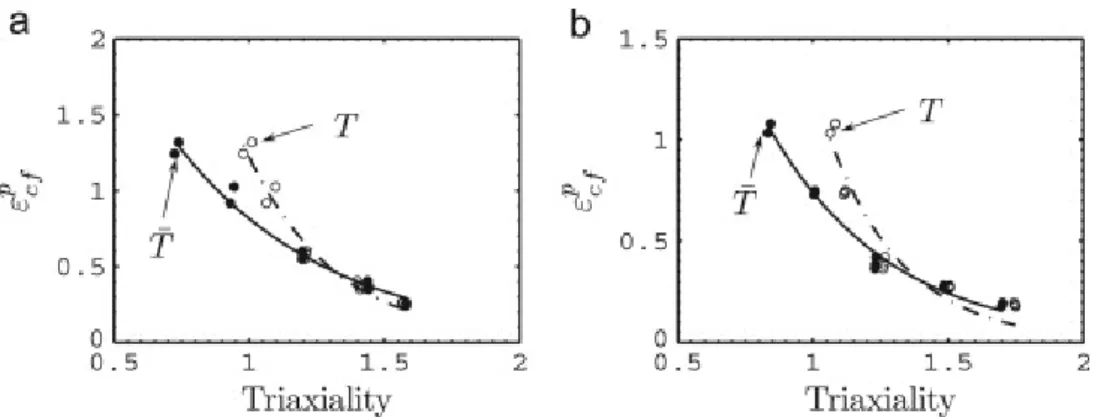
The effect of stress triaxiality on the ductile failure is illustrated in Figure 2.3 for a medium strength steel (a) and a high strength steel (b) [14]. The equivalent plastic strain at failure in the centre of the specimen (ϵp_cf) is plotted against the stress triaxiality. It can clearly be seen that the ductility decreases significantly with increasing stress triaxiality. In this plot T is the stress triaxiality at failure and ¯T is the average stress triaxiality during the test. As ductile damage is

a progressive phenomenon it is interesting to look at the evolution of the stress triaxiality over the entire loading history.

The evolution of the stress triaxiality as a function of plastic strain is shown in Figure 2.4 [14]. The stress triaxiality is plotted against the equivalent plastic strain at the centre of the specimen (ϵpc) and a/r is the ratio of the notch depth to the notch radius. The notch depth

(a) was kept constant at 3 mm while the notch radius was varied between 1 and 15 mm. The points on the graph are where the specimens failed. It can be seen that the stress triaxiality quickly rises to a certain value as plasticity starts to develop. This value is greater for a smaller notch radius. After this, the stress triaxiality continues to rise for specimens that started with

(29)

Figure 2.3: Influence of stress triaxiality on the equivalent plastic strain at failure in the middle of the specimen. Figure (a) shows a medium strength steel and figure (b) shows a high strength steel [14]

low stress triaxiality while it remains constant or drops slowly for specimens that started with higher stress triaxiality.

Figure 2.4: Stress triaxiality evolution during loading for different notch radii, with a/r = 0.2, 0.6, 1.2, 2.0, 3.0 [14]

The stress triaxiality also determines the mechanism in which the strain becomes localised and void coalescence occurs. There are two main mechanisms in which void coalescence can take place [13, 15]. The first is the local necking of the ligaments between voids once these voids have grown significantly, which dominates when the stress triaxiality is high. The second is shear localisation of the strain in ligaments between voids that have only grown a relatively small amount, which occurs when stress triaxiality is low. The stress triaxiality at which the transition between these mechanisms occurs is material dependant and not well defined. The transition stress triaxiality typically used in literature ranges between 0.3 and 0.8 [4, 16, 17, 18]. In case coalescence occurs by the first mechanism, the influence of the stress state on the material

(30)

10 2.3. DUCTILE FAILURE

behaviour can be accurately described by only using the stress triaxiality [17]. In case the second mechanism occurs, the stress triaxiality alone is no longer sufficient to describe the effect of the stress state and the Lode angle should be taken into account.

The effect of the stress triaxiality and Lode angle on the equivalent plastic strain at failure can be visualised in a fracture locus. This is shown in Figure 2.5 [4]. The exact values depend on the material but the trends shown are valid for all typical metals, except for the reduction in ductility when the Lode angle is negative. It can be seen that for high stress triaxiality values the effect of the Lode angle is negligible. Conversely, for low stress triaxiality levels, the effect of the Lode angle becomes very pronounced. In the case of low stress triaxiality, for

¯

θ = 1, corresponding with axially symmetric tension, ductility is high. This can be explained

as here there is not a lot of void growth, while void deformation by shearing is also low. Both mechanisms leading to void coalescence are thus slow in this stress state, and the material will be able to deform significantly before coalescence occurs. At generalised shear stress states (¯θ = 0)

with low stress triaxiality void coalescence will occur relatively quickly by shear localisation and hence the ductility is severely decreased compared to the case with axially symmetric tension.

Figure 2.5: 3D fracture locus showing the effect of stress triaxiality (η) and Lode angle (¯θ) on

the equivalent plastic strain at failure ( ¯ϵf) [4]

2.3.2 Fracture toughness testing

The fracture toughness behaviour of a material is commonly measured by applying a gradually increasing displacement to a test specimen that contains a sharp crack that was introduced prior to the test, for instance by fatigue precracking [5]. During the test, a measure for the crack

(31)

driving force and the growth of the crack are measured. Common measures for the crack driving force are the crack tip opening displacement (CTOD) or the J-integral for ductile failure. The required crack driving force to grow a crack by a certain amount can then be visualised in a crack growth resistance curve (R-curve), as shown in Figure 2.6 [19].

Figure 2.6: A crack growth resistance curve [19]

Three standardised tests for obtaining resistance curves are discussed: compact tension (CT), single edge notched bending (SENB) and single edge notched tension (SENT). The geometries of these specimens are shown in Figure 2.7 [5], the geometry for the SENT specimen is the same as the SENB specimen (but it is noted that the dimensions would be different). In CT and SENB tests the crack tip is loaded in bending, which induces a very high stress triaxiality at the crack tip. In SENT tests the crack tip is loaded in tension which induces a lower stress triaxiality at the crack tip, but still above the transition value discussed in subsection 2.3.1. This difference in stress triaxiality will cause failure to occur more quickly in CT and SENB specimens than in SENT specimens. For applications where defects are loaded in tension, such as pipelines, SENT tests are preferred as CT or SENB tests would substantially overestimate crack growth [5].

2.4 Conclusion

In this chapter ductile failure was discussed, by looking at the working principle, important parameters and testing methods. The following provides a brief overview of the current chapter: • The micromechanical mechanism of ductile failure is characterised by three stages: void

nucleation, void growth and void coalescence.

• The stress state is described by two dimensionless invariants: the stress triaxiality (η) and the normalised Lode angle (¯θ).

(32)

12 2.4. CONCLUSION

Figure 2.7: Possible specimen geometries for fracture toughness tests

• Void nucleation and void growth are both promoted by high levels of stress triaxiality, leading to decreased ductility. At high values of stress triaxiality, the coalescence occurs by local necking of the ligaments between voids, while at low values of stress triaxiality, coalescence occurs by local shearing.

• The effect of the normalised Lode angle is only pronounced at a low stress triaxiality level. In this case, void coalescence is promoted by generalised shear stress states (¯θ = 0).

• The resistance of material under a certain stress state against ductile failure can by de-scribed by a tearing resistance curve. In such a curve the required crack driving force to grow a crack by a certain amount is visualised. The resistance curve is obtained through standardised tests. This thesis focusses on SENT tests.

(33)

3

Gurson-based damage models

3.1 Introduction

The Gurson model is an early micromechanics-based model developed to describe ductile failure. It has received multiple extensions and modifications by various authors and continues to be further developed [7]. These Gurson-based models are widely used today. The original Gurson model and a few key modifications will be discussed below.

3.2 Original Gurson model

The original model developed by Gurson was based on the behaviour of a rigid-plastic material containing a single spherical void that doesn’t change in shape, but does change in size upon loading [20]. The material is subjected to a homogeneous strain rate at its boundaries. Gurson proposed a modification of the von Mises yield surface by introducing the hydrostatic stress and a new parameter called the void volume fraction (f ). This parameter is the ratio of the volume of the spherical void and the volume of the matrix material cell. This cell is initially a cube, where the length of a side should be approximately equal to the average spacing between large inclusions in the material [21]. The material is thus built up from these cubes, each having their own void volume fraction. This new yield surface was defined as

Φ(σe, σm, σf, f ) = ( σe σf )2 + 2f cosh ( 3σm 2σf ) − 1 − f2 _{= 0} _(3.1) 13

(34)

14 3.3. GURSON-TVERGAARD-NEEDLEMAN MODEL

where σf is the flow stress and f is the void volume fraction. It can easily be seen that if the void

volume fraction is 0, no voids are present and the yield surface reduces to the von Mises yield surface. When f is 1 the cell is completely void and thus has cannot carry any load anymore. This model doesn’t account for the interaction between voids or strain localisation however.

3.3 Gurson-Tvergaard-Needleman model

The first adjustment was made by Tvergaard, who added three parameters (q₁, q2, q3) to the

Gurson model [22, 23]. He analysed the micromechanics of a material containing periodically distributed voids with cell model calculations. The parameter q3 has been accepted to be equal

to q2

1. These parameters are necessary because Gurson approximated the plastic dissipation with

a Taylor series and only calculated the first order terms [24]. The parameter q1 is a material

property and can accurately account for the effect of this approximation for quasistatic loading conditions [24]. In case of dynamic loading the stress triaxiality can become very large and q₁ would also need to be dependent on the stress triaxiality. This might cause problems with the convexity of the yield function, so the Gurson model is unsuitable to predict dynamic failure. Two years later the model was modified a second time by Tvergaard and Needleman to be able to predict the effects of void coalescence [25]. To do this the void volume fraction was modified to artificially increase after a critical void volume fraction is reached, at which void coalescence starts to occur. This model is called the Gurson-Tvergaard-Needleman or GTN model and is described by the following equations:

Φ(σe, σm, σf, f∗) = ( σe σf )2 + 2q1f∗cosh ( 3q2σm 2σf ) − 1 − q2 1f∗2= 0 (3.2) f∗(f ) =            f if f < fc fc+ f_u∗− fc fF − fc (f − fc) if fc≤f ≤ fF f_u∗ if fF <f (3.3)

where f∗ is the modified void volume fraction, fc is the critical void volume fraction at which

coalescence starts, fF is the final void volume fraction at which failure occurs and fu∗ is the

ultimate value of the modified void volume fraction which is taken as 1

q1.

Void coalescence is not physically described in the GTN model. Instead the growth of the void volume fraction is artificially accelerated when a critical void volume fraction is reached, as described by Equation 3.3. fcis assumed to be a material property, to be empirically determined.

This adds another constant to the model that needs to be calibrated, and it has been shown that it causes a non-uniqueness problem in calibration [26], as further explained in section 3.5.

(35)

CHAPTER 3. GURSON-BASED DAMAGE MODELS 15

3.4 Void volume fraction evolution

The Gurson model also needs to include equations to describe the three stages of ductile failure, namely void nucleation, growth and coalescence. These are used to simulate the evolution of the void volume fraction during a certain deformation. The evolution of the void volume fraction can be split into two contributions: the part due to the nucleation of new voids and the growth of existing voids:

˙

f = ˙fnucleation+ ˙fgrowth (3.4)

The nucleation is controlled by the change in stress and strain as follows [27]: ˙

fnucleation= A ˙ϵpeq+ B( ˙σf + ˙σm) (3.5)

where A and B are parameters to be determined and ˙ϵpeq is the equivalent plastic strain rate.

Usually the nucleation is assumed to be either strain-controlled with B = 0 or stress-controlled in which case A = 0 [26] . Strain controlled nucleation is usually chosen in studies because it is easier to handle in the finite element implementation [26], and will also be used in this work. The parameter A is then the void nucleation rate and is assumed to follow a normal distribution [28]. It has the following expression:

A = fN SN √ 2πexp [ −1 2 ( ϵpeq− ϵN SN )2] (3.6) where fN is the volume fraction of void nucleating particles, ϵN is the mean void nucleation

strain and S_N is corresponding standard deviation.

The increase in void volume fraction due to the growth of existing voids is described using conservation of mass as:

˙

fgrowth= (1− f)˙ϵpii (3.7)

where ˙ϵp_ii is the plastic hydrostatic strain.

3.5 Complete Gurson model

The assumption that fc is a material property is not realistic. It has been shown that fc is

instead a strong function of the initial void volume fraction f0 and also depends (less strongly)

on the stress triaxiality and strain hardening exponent. Therefore, it has been suggested to determine fc as a function of f0 [29]. A large problem with taking fc as a function of f0 is

that it has also been shown that f0 and fc cannot be uniquely determined from tensile tests,

which is the method commonly used in literature [26]. To solve this problem the GTN model was modified to the complete Gurson model (CGM), which automatically predicts the start of void coalescence based on the principal stresses and strains [26]. This means that f_c is not a constant that should be calibrated any more, but is rather treated as a field quantity.

(36)

16 3.6. PARAMETER IDENTIFICATION

This is achieved by incorporating Thomason’s plastic limit load criterion [30]. This criterion compares the stress required for homogeneous deformation with the stress required for localised deformation. At the start of deformation the stress required for homogeneous deformation will be lower and thus homogeneous deformation will occur. However, at a certain point, the stress required for homogeneous deformation will become equal to the stress required for localised deformation, and void coalescence will start to occur. This point is described by [30]:

σ1 σf = ( α ( 1 r − 1 )2 +√β r ) (1− πr2) (3.8) r = 3 √ 3f 4πeϵ1+ϵ2+ϵ3 √ eϵ2+ϵ3 2 (3.9) where σ1 is the maximum principal stress, ϵ1,2,3 are the principal strains, α and β are fitting

constants. These constants were fitted to be α = 0.12 + 1.68n, where n is the Ramberg-Osgood hardening exponent, and β = 1.2 when used in the complete Gurson model [26].

When the condition in Equation 3.8 occurs in an integration point in the material, the value of fc in this point is taken as the void volume fraction at that time for this integration point.

In this way f_c is automatically determined for every integration point of the material during simulations. This is in contrast to the GTN model, where fc is a material property and is

determined before the simulations by fitting data from tensile tests. It should be noted that the void volume fraction at final failure is not automatically determined by the CGM. Thus, the parameter fF should still be calibrated, and takes on the same value for all integration points.

A drawback of the Complete Gurson model is that it cannot accurately predict the damage evolution, and thus the stress required for continued plastic deformation and strain at failure, for stress states with low stress triaxiality. This can be explained because coalescence no longer occurs by internal necking of ligaments between voids, as assumed in the CGM, but by shear localisation in the ligaments. In other words, the CGM predicts coalescence once the voids have grown to a critical size, whereas in states of generalised shear coalescence occurs earlier without much void growth. This problem has been addressed by introducing the effect of the Lode angle into the model [31]. This modification will not be used in this thesis, as stress states with high triaxiality are present at the crack tip in SENT specimens, on which the CGM will be applied. The calibration procedure of the CGM will use experiments with notched round bars, in which a high stress triaxiality is also present.

3.6 Parameter identification

In order to apply the complete Gurson model (CGM), 7 parameters (q1, q2, f0, fF, fN, ϵN,

SN) need to be identified alongside the idealised damage-free true stress-strain behaviour of

(37)

CHAPTER 3. GURSON-BASED DAMAGE MODELS 17

calculated). The first set of model parameters are the material parameters q1 and q2 introduced

by Tvergaard [22, 23], where they are suggested to be 1.5 and 1 respectively for all ductile metals. They have later been found to be material dependant and were calibrated by Faleskog et al. as a function of the strength (σ0/E), where σ0 is the yield strength and E the Young’s modulus,

and the Hollomon strain hardening exponent (N ) of the material.[21]. In the mentioned paper the following relation is used to approximate the true stress-strain material behaviour:

ϵ =    σ0 E if σ < σ0 σ0 E ( σ σ0 )1/N if σ_{≥ σ}₀ (3.10)

The calibrated values are shown in Table 3.1.

Table 3.1: Calibrated values of q₁ and q₂ [21]

σ0/E = 0.001 σ0/E = 0.002 σ0/E = 0.004 Hardening N q1 q2 q1 q2 q1 q2 0.025 1.88 0.956 1.84 0.977 1.74 1.013 0.05 1.63 0.950 1.57 0.974 1.48 1.013 0.075 1.52 0.937 1.45 0.960 1.33 1.004 0.1 1.58 0.902 1.46 0.931 1.29 0.982 0.15 1.78 0.833 1.68 0.856 1.49 0.901

The second set is the initial void volume fraction (f0) and nucleation parameter (fN). These

are usually determined by quantitative microscopical analysis of the undamaged material, using the inclusion volume fraction [11, 32, 33]. But this approach is only approximately correct as not all inclusions will nucleate voids. Therefore, these parameters should be calibrated using the macroscopic material behaviour [26, 34]. In this work these parameters will be determined with a surrogate-based analysis comparing numerical and experimental results as explained in chapter 5.

The remaining parameters are fc, fF, ϵN and SN. In literature, the parameters ϵN and SN are

often fixed to 0.3 and 0.1 respectively [11]. The void volume fraction at failure (f_F) can be approximated by the following relation [26].

fF = 0.15 + 2f0 (3.11)

However, this equation is only valid for materials with large inclusions where all voids are nucleated at low strain levels.

The void volume fraction at the onset of void coalescence (fc) is not viewed as a material property

but rather as a field quantity in the complete Gurson model, as discussed in section 3.5. It is determined by the plastic limit load criterion for coalescence by Thomason [30].

(38)

18 3.7. CONCLUSION

3.7 Conclusion

In this chapter, Gurson-based damage models were discussed, with particular attention paid to the complete Gurson model (CGM). The following provides a brief overview of the current chapter:

• The original Gurson model proposed a modification to the von Mises yield surface, by introducing the hydrostatic stress component and a new parameter called the void volume fraction (f ).

• Three material dependant parameters were added to the original Gurson model by Tver-gaard. Needleman modified the void volume fraction to artificially increase after a critical void volume fraction (fc) is reached, to model the effect of void coalescence. These

modi-fications are combined in the Gurson-Tvergaard-Needleman model. fc is assumed to be a

material property.

• When modified again to the complete Gurson model, fc is treated as a field quantity

instead of a material property. Thomason’s plastic limit load criterion is used to predict

fc for each integration point during simulations.

• Seven parameters need to be identified in order to use the CGM, alongside the damage-free true stress-strain curve of the material. Based on the tensile properties of the material, q1

and q₂ can be determined from calibrated values which were tabulated by Faleskog. • The CGM can not predict the damage evolution for stress states with low stress triaxiality,

where void coalescence occurs by shearing. There exists a modification that solves this issue, but this modification is not used in this thesis, as only tests which induce a high stress triaxiality are modelled.

(39)

Part II

Methods and results

(40)

4

Experiments

4.1 Introduction

In this chapter the performed experiments are described. These experiments are performed in order to compare the results with results from simulations. This comparison will be employed in the calibration procedure of the CGM, described in chapter 5. The experimental results will also be used to estimate the anisotropy of the material. The test specimens are described in section 4.2. The test setup is briefly described in section 4.3. Next, a more detailed look is taken at the digital image correlation system in section 4.4 and the diameter reduction image analysis in section 4.6. Finally, the results of the experiments are described in section 4.7.

4.2 Test specimens

4.2.1 Material

The test specimens that are used for the calibration procedure were machined out of steel grade L480. These specimens were extracted from a pipe with outer diameter of 941 mm and nominal wall thickness of 17.1 mm. The SENT test specimens were extracted from the same pipe. The SENT tests were performed within the scope of another research project [1], where the are described in detail.

(41)

CHAPTER 4. EXPERIMENTS 21

4.2.2 Geometry and dimensions

The performed experiments comprise of tensile tests of three notched round bar (NRB) spec-imens, and one rounded smooth specimen. The smooth specimen is used to obtain the true stress-strain material curve. The NRB specimens are used to calibrate the CGM. The calibra-tion procedure employed is described in chapter 5. Figure 4.1 presents the dimensions of the smooth specimen and Figure 4.2 the dimensions of the NBR specimens.

Figure 4.1: Geometry of the smooth specimen (dimensions in mm)

Figure 4.2: Geometry of the notched round bar specimens (dimensions in mm)

4.2.3 Influence of geometry on stress triaxiality

NRB specimens with different radii are chosen to induce different levels of stress triaxiality. The range of stress triaxiality should include the stress triaxiality present at the notch tip in SENT specimens. This starts at around 1 and evolves to around 1.7 as the test progresses, after which it starts to decrease again [35]. The calibrated CGM should be valid for all values of stress triaxiality higher than the transition value (0.3 - 0.8) where the influence of the Lode angle can be neglected, as described in subsection 2.3.1. The notch radii in the longitudinal direction are chosen to be 1.2, 2 and 6 mm. The smallest cross sectional radius is chosen as 3 mm, and the nominal cross sectional radius of the bar as 5 mm. With these values the stress triaxiality (η), at the centre of the cross section inside the notch, can be estimated using Bridgman’s formula [10]: η = 1 3+ ln ( 1 + ρ 2r ) (4.1) where ρ is the minimum cross sectional radius of the specimen and r is the notch radius in the longitudinal direction. The estimated stress triaxiality is 1.14 for r = 1.2 mm, 0.89 for r = 2 mm and 0.56 for r = 6 mm. These values are valid for the onset of plasticity.

(42)

22 4.2. TEST SPECIMENS

It has been observed that the stress triaxiality changes with increasing equivalent plastic strain [14] (see Figure 2.4). Therefore, preliminary simulations are performed using the finite elements software ABAQUS © (version 6.14). In these simulations, the effect of the strain hardening exponent (n) on the stress triaxiality is examined.

A quarter of the NRB specimens is simulated, using symmetry conditions. A displacement is imposed on the top face while the bottom face is constrained. The elastic material response is defined by a Young’s modulus (E) of 210 GPa and a Poisson’s ratio (ν) of 0.3. The plas-tic response is defined by a yield stress at 0.2% plasplas-tic strain (R_p0.2) of 592.84 MPa, and the Ramberg-Osgood relationship [36]: ϵp = K (_σ E )n (4.2) where ϵp _{is the plastic strain and σ the true stress. The simulations were performed for n = 10}

and n = 20, with K determined by the definition of Rp0.2.

Figure 4.3 illustrates the influence of the r and n on the stress triaxiality evolution versus the plastic strain, in the element at the centre of the cross section inside the notch. The stress triaxiality at zero plastic strain is close to the values predicted by Bridgman’s formula, as illustrated in Table 4.1. The strain hardening exponent has no influence on these stress triaxiality values, as they are determined at the onset of yielding, so no strain hardening has occurred. The stress triaxiality is higher for a sharper notch. The stress triaxiality quickly rises as plasticity starts to develop. With further increasing plastic strain the stress triaxiality continues to rise for r = 6 mm while it remains constant for r = 2 mm and drops for r = 1.2 mm. Furthermore, it is found that the stress triaxiality is higher for n = 20 than for n = 10, with a more pronounced effect for sharper notch radii.

Figure 4.3: Influence of r and n on stress triaxiality evolution

From the results of the preliminary simulations, it can be concluded that the presupposed stress triaxiality range, corresponding to that present at the crack tip of an SENT specimen (1 - 1.7), can be induced by the notch radii of 1.2, 2 and 6 mm.

Ductile fracture modelling of Single Edge Notched Tension (SENT) tests using the complete Gurson damage model

damage model

Tension (SENT) tests using the complete Gurson

Ductile fracture modelling of Single Edge Notched

Counsellor: Vitor Soares Rabelo Adriano

Supervisors: Prof. dr. ir. Stijn Hertelé, Prof. dr. ir. Wim De Waele

damage model

Tension (SENT) tests using the complete Gurson

Ductile fracture modelling of Single Edge Notched

Counsellor: Vitor Soares Rabelo Adriano

Supervisors: Prof. dr. ir. Stijn Hertelé, Prof. dr. ir. Wim De Waele

Preface

Ductile fracture modelling of Single Edge

Notched Tension (SENT) tests using the

complete Gurson damage model

Ben Van Raemdonck

Ductile fracture modelling of Single Edge Notched

Tension (SENT) tests using the complete Gurson

damage model

Contents

List of Figures

List of Tables

List of Symbols

1

Introduction

1.1

Research context

1.2

Objectives

1.3

Outline

Part I

Literature review

2

Ductile failure modelling

2.1

Introduction

2.2

Plasticity theory

2.3

Ductile failure

2.4

Conclusion

3

Gurson-based damage models

3.1

Introduction

3.2

Original Gurson model

3.3

Gurson-Tvergaard-Needleman model

3.4

Void volume fraction evolution

3.5

Complete Gurson model

3.6

Parameter identification

3.7

Conclusion

Part II

Methods and results

4

Experiments

4.1

Introduction

4.2

Test specimens