RIVM Report 861004001/2007
Uncertainty analysis and parameter optimisation in
early phase nuclear emergency management
A case study using the NPK-PUFF dispersion model
C.J.W. Twenhöfel M.M. van Troost S. Bader Contact: C.J.W. Twenhöfel RIVM chris.twenhofel@rivm.nl
This investigation has been performed by order and for the account of the Director General of RIVM, within the framework of project S/861004 (MUSHROOM)
© RIVM 2007
Parts of this publication may be reproduced, provided acknowledgement is given to the 'National Institute for Public Health and the Environment', along with the title and year of publication.
Abstract
Uncertainty analysis and parameter optimisation in early phase nuclear
emergency management
The determination of radiation doses received after a nuclear accident can be improved if model calculations are combined with an analysis of radiological measurements in the local environment of the release point. Dose estimates in the early accident phase are currently based on model calculations only. These calculations have large uncertainties. This was demonstrated in a case study by the National Institute for Public Health and the Environment (RIVM).
Uncertainty in model calculations after a nuclear accident makes it difficult for a decision maker to decide on counter measures to protect the population. For this reason RIVM will use measurements of the national radioactivity monitoring network to improve the model calculations. Important uncertain model input parameters were shown to be the release rate and some meteorological parameters.
The case study demonstrated that a small number of radiological measurements in the early phase of the release are sufficient to significantly improve the determination of radiation doses. It is therefore recommended to implement the method in the Back Office for Radiological Information (BORI) of RIVM. BORI estimates the radiological consequences for men and environment during and after a nuclear or radiological accident.
This research is part of the strategic research program of RIVM in the area of quantitative risk assessments.
Key words: nuclear emergency management, data assimilation, quantitative risk estimates, dispersion model, parameter optimization
Rapport in het kort
Onzekerheidsanalyse en parameteroptimalisatie in de vroege fase van de
kernongevallenbestrijding
De opgedane stralingsdosis na een kernongeval is beter te bepalen door modelberekeningen te combineren met een analyse van radiologische metingen in de directe omgeving van de lozing. Dosisschattingen die alleen op basis van modelberekeningen zijn gemaakt, zoals nu gebeurt, bevatten meerdere grote onzekerheden. Dit blijkt uit een casestudie van het Rijksinstituut voor Volksgezondheid en Milieu (RIVM).
Onzekerheid in modelberekeningen na een kernongeval maakt het de beleidsmakers lastig te beslissen welke maatregelen nodig zijn om de bevolking te beschermen. Daarom gaat het RIVM metingen van het nationale radiologische meetnet in Nederland gebruiken om de modelberekeningen te verbeteren. De belangrijkste onzekere variabelen zijn beperkt tot de lozingshoeveelheid en een aantal
meteorologische parameters.
Het onderzoek toont aan dat al in een vroeg stadium van het ongeval met slechts een klein aantal radiologische metingen een significante verbetering van de dosisberekening mogelijk is. Het verdient daarom aanbeveling deze methodiek te implementeren in het Back Office voor Radiologische
Informatie (BORI) van het RIVM. Het BORI heeft de taak in te schatten wat de radiologische gevolgen van een kernongeval zijn voor mens en omgeving.
Dit onderzoekt maakt deel uit van het strategisch onderzoeksprogramma van het RIVM (SOR) op het gebied van kwantitatieve risicoanalyse.
Trefwoorden: kernongevallenbestrijding, data-assimilatie, kwantitatieve risicoanalyse, dispersiemodel, parameteroptimalisatie
Contents
Summary 9
1 Introduction 11
2 Methods 13
2.1 Concept of the data assimilation method 13
2.2 Concept of uncertainty analysis 14
2.3 Case definitions 15
2.4 Calculation endpoints and gamma station layout 19
3 Proof of concept 23
3.1 Sensitivity analysis 23
3.2 Optimisations in two dimensions 25
3.3 Optimising the multi-dimensional parameter space 26
4 Case study uncertainty 29
4.1 Standard model output for the reference case 29
4.2 Reference case 29
4.3 Case variations 32
4.4 Cases with minimum and maximum knowledge 33
4.5 Ranking parameters 35
5 Case study data assimilation 39
5.1 Mapping MVT variability 39
5.2 Optimisation of parameters by MVT ranking 42
5.3 Optimisation using alternative geometries 45
6 Discussion and conclusions 49
References 51
Appendix 1 The NPK-PUFF dispersion model 55
Summary
A new method is developed and evaluated that can be used to improve the rapid assessment of radiation exposure in nuclear emergencies. The method combines meteorological dispersion calculations of the NPK-PUFF atmospheric dispersion model with sparsely available measurement data in the first phases of a nuclear accident to optimise model input parameters and improve the model output.
In the Netherlands radiological measurements are available in real time from the Dutch National Radioactivity Monitoring network (NMR) and from mobile measuring stations of RIVM, the Department of Defence and the local fire brigades. The real time availability of these measurements allows their use for a model optimisation method.
Uncertainty in the NPK-PUFF model results is dominated by a highly uncertain release rate and meteorological parameters. In practical emergency management, uncertainty estimates in model parameters are to a large extent based on expert judgement. Uncertainty is therefore not a matter of variability but of unknown inputs. For a typical scenario, prognosticated at the start of release, the model results can be within a range of several orders of magnitude. In this study we refer to this situation as the “minimum knowledge” case. An uncertainty analysis on the NPK-PUFF model input parameters revealed significant contributions from the release rate, mixing height, wind speed and wind direction. During rainfall, the precipitation rate has to be included as well. In practical cases the uncertainty analyses and the following parameter optimisation method can be limited to these five important parameters. Uncertainty in the model input parameters gives rise to a range of possible model outcomes. This interferes with a simple yes or no decision with respect to countermeasures; the probability of exceeding an intervention level enters the operational emergency management domain. Using the selected parameters from the uncertainty analysis a method was tested to optimise input parameters based on radiological measurements. We used the Model Validation Tool (MVT) of RIVM as a measure of conformity between model output and radiological measurements. The cases were constructed following operational examples and several spatial designs of the monitoring network were evaluated. We optimised dispersion model output for the early phase of nuclear accident management, represented by the first hour of monitoring data. With the exception of high stack releases and releases under conditions of (very) low wind speed all cases were easily optimised using the simulated radiological data. This was also the case for the spatial design of the NMR, although the number of variable model input parameters had to be limited to four (or five including precipitation): release strength, wind speed, wind direction and mixing height.
It is demonstrated that the optimisation method worked well, when applied to the simulated cases, i.e. the reliability of dose estimates improved significantly. Based on the new set of optimised model input parameters a recalculation of the dispersion model also improved the radiological prognosis. It is therefore recommended to implement the optimisation method as an extension to the current model capabilities of the Back Office for Radiological Information (BORI) at RIVM and to study the possibilities to extend its application to longer time scales (later phases) and spatial coverage.
1
Introduction
During large scale nuclear accidents an effective countermeasure strategy to protect the population and the environment in the early phase of emergency management, is generally based on quantitative risk estimates for the current situation (diagnosis) and the near future (prognosis); see e.g. (1-3). In view of the large social and economical impact of countermeasures, not only a prompt implementation but also the reliability of the underlying risk estimates is of crucial importance. In this study we have the objective to improve these quantitative risk estimates for the current situation and the near future in the very early phase of nuclear emergency management.
In off-site consequence assessments extensive use is made of models and data from radiological measuring networks and (mobile) environmental measurement facilities. These information sources have specific advantages and limitations as well. Model results give excellent geographical overviews of the radiological situation in the target area as a function of time, i.e. of the past, the present and the future. Models are further well suited of signalling when and where intervention contours or operational action levels are exceeded. An important disadvantage is the high level of uncertainty associated with early phase radiological model calculations due to uncertainty in the model input parameters and limitations in the conceptual model. Radiological measurements appear much more reliable when compared to model results. However, measurements have severe limitations in time, space and in the measurable quantity. Intervention levels (ILs), for example, are seldom expressed in terms of measurable quantities. An adequate description of the accident situation thus demands a considerable interpretation and calculation effort. Also, the availability of measurement results lags a certain time interval behind of the actual situation.
When fast and reliable results from the risk analyses efforts are required, the two techniques must be combined. In complex situations, as in case of nuclear accidents, a spectrum of radio nuclides is released in complicated time dependant release profiles and uncertain meteorological conditions. A fast and reliable method for performing quantitative risk estimates based on a combined approach of modelling and measurement capabilities is not currently at hand in these situations. Techniques of combining measurements and model calculations generally fall under the domain of data assimilation. Internationally some initiatives have been taken to design and test data assimilation schemas for nuclear risk estimates (4-6). We followed an approach based on an optimisation technique of the model input parameters. The methodology was introduced earlier in (7, 8).
In this report a proof of concept and a case study on uncertainty analysis and data assimilation for early phase nuclear emergency management are presented. The proof of concept is based on real, but non-radiological, dispersion and measurement data, the uncertainty and data assimilation case study uses simulated radiological measurement data generated by the dispersion model itself to study uncertainty and the optimisation of quantitative risk estimates. This latter analysis has the important advantage that release conditions and atmospheric dispersion characteristics are well under control. The proof of concept is described in chapter 3, the uncertainty and data assimilation studies are described in chapter 4 and 5. In chapter 2 the methodology and the case definitions are presented.
2
Methods
This chapter introduces the concepts of the data assimilation and the uncertainty analysis techniques. These techniques are applied in the case study on uncertainty and parameter optimisation; the subject of this report, described in chapter 3 to 5. Section 2.3 and 2.4 describe the case definitions and the spatial layout of the measurements.
2.1
Concept of the data assimilation method
Data assimilation is aimed at a reduction of uncertainty in the model results of the atmospheric dispersion model, thereby optimising the deterministic analysis, including the prognosis. For this, radiological measurements are included into the mathematical formalism. Examples of earlier studies on the subject are, e.g. found in (9-11). The technique, is often based on an implementation of a Kalman filter (12-15). Disadvantages of the Kalman filter are the complexity of the mathematical calculations and the vast data volume required for the optimisation process. We concentrated on the early release phase of accident management when monitoring data is sparsely available and fast calculations are required in order to support the emergency management process. We therefore followed a different approach. We optimised the input parameters of the atmospheric dispersion model based on observed radiological data. The method starts with an expert judgement on the plant status and the meteorological conditions around the release location on which a release scenario is defined. During the release period radiological measurements become available and are compared to the model results. In the Netherlands, these measurements are provided by the National Radioactivity Monitoring Network (NMR) (16) or they come from mobile measuring stations. We used ambient dose (equivalent) rate, H*(10), measured over a certain period in time. These measurements are easily performed and available from various sources in (almost) real-time.
Figure 1. Flow chart of the data assimilation technique using RIVM’s Model Validation Tool (MVT) and IMSL fitting procedure (BCPOL) to establish an improved prognosis from the dispersion modelling.
PLANT STATUS NPK-PUFF MODEL HIRLAM ECMWF LOCAL METEO MEASUREMENTS MODEL Validation Tool INPUT MODEL PARAMETERS MINIMISATION ROUTINE (IMSL)
The match between the model results and the observed data is delivered by the rank value of RIVM’s Model Validation Tool (MVT). The MVT integrates up to 10 statistical parameters to assess the spatial and temporal comparability of measurements and models. An optimisation of the input parameter values minimises the rank value of the MVT function. The conceptual method is shown in Figure 1. The NPK-PUFF atmospheric dispersion model and the MVT are described in Appendix 1 and 2. The minimisation procedure, BCPOL, is taken from the IMSL Math Library (17) and is suited for minimisation of non-smooth functions with simple bounds using a direct search complex algorithm, see e.g. (18). The minimisation routine samples the predefined input parameter space and starts model calculations based on the sampled input parameters. The MVT rank value is determined and optimised by the minimisation routine. Dependent on a predefined tolerance level or a maximum number of model runs (up to 500 can be defined) the iterative process will come to an end as significant improvements are not achieved by further iterations. This minimisation procedure was especially chosen for its robustness.
2.2
Concept of uncertainty analysis
In (19) a number of distinct categories of uncertainty, influencing the reliability of model predictions are identified. In this study we respectively assume a sufficient level of confidence in the assessment problem, the conceptual model and the model implementation. Of interest in practical emergency management analyses is the uncertainty in the estimation of the input parameter values, i.e.: the source (scenario) and the physical transport (meteorology, transfer factors, deposition process) (19).
In general two types of uncertainty can be identified in deterministic models: a stochastic variability, leading to uncertain probabilistic answers and uncertainty caused by a lack of knowledge of certain input parameters, which leads to imprecise deterministic answers. In reality both type of uncertainty are present in practical cases. However, the lack of knowledge by far dominates uncertainty in the assessment problem of nuclear accident management. This suggests a model output not of variability but of alternative possible true answers. The resulting model output is represented by a cumulative distribution function (cdf), P(Y≤y); the probability of finding a model result Y below value y. Technically we accomplished this by generating a random sample of certain size n (we used 500 in the final analysis) of n-tuples of input parameter values according to the joint probability distribution of these parameters. The corresponding n model output values are then ordered on increasing numerical value so that the cdf can be deduced. We used Latin Hypercube (LHC) sampling for the n-tuples (19). This method overpopulates the low probability regions of the individual probability functions of the parameters. Since the estimation of initial parameter uncertainty is primarily based on expert judgement of the radiological advisor the cdf, P(Y≤y) becomes a subjective probability function. Values are generally referred to as subjective confidence level. The general approach to the uncertainty analyses is (19):
1. Identify all parameters that are potentially important contributors to uncertainty; 2. Specify the maximum conceivable range of alternative values;
3. Construct (subjective) probability functions for the parameter values;
4. Derive quantitative statements on the effect of parameter uncertainty on the model prediction; 5. Rank parameters with respect to their contribution to the uncertainty in the model prediction. The first step is known as a sensitivity analyses. It concerns with the question how the model output reacts to variations in the nominal values of the model parameters, the initial conditions and the release scenario. A sensitivity analysis is addressed in section 3.1. The last two steps are associated with an
uncertainty analyses. The computer programme UNCSAM (20) of RIVM was used to sample the input parameters according to the user-defined probability functions. It was also used to calculate the ranking of the input parameters with respect to its contribution in the overall uncertainty. The uncertainty analysis is described in chapter 4.
2.3
Case definitions
This study is based on cases defined by the Kincaid data set, representing real atmospheric dispersion data and several modelled releases using the NPK-PUFF model. These latter cases allowed us to examine uncertainty and the performance of the data assimilation technique for specific release characteristics and meteorological conditions. A complete case specification (scenario) consists of a source term (release) description, meteorological conditions and dispersion model parameters, for short we will use the term parameter for all these inputs without distinction. A total of nine cases are used in this study.
Kincaid data set
The Kincaid data set (21) represents a high stack release from a coal powered electricity production facility in Illinois (USA). It represents a well known and real, but non-radiological data set. It consists of 350 hours of observations of SF6 tracer gas, in the vicinity of the electricity production facility. Data
was accumulated in periods of 24 days during 1980 and 1981. The Kincaid data set represents releases at high altitudes (187 m) with a considerable heat content (several hundreds of MWs), which results in an effective release height of about 700 m (22). The data set comprises detailed meteorological data and observations of air concentrations of SF6 in a ring geometry at several distances up to about 55 km.
We used the Kincaid data set to perform sensitivity studies on model parameters and provide a measure of conformity between the daily time-integrated air concentration from the model calculations and the measurement data. The time-integrated air concentrations were taken from a particular day from the Kincaid data set (16 May 1981). This case is used in the proof of concept in chapter 3.
Reference case
The reference case defines a modelled accident with realistic off-site consequences. We used the well known PWR5 accident (23). The case consists of a ground release (10 m) of radio nuclides over a time period of 4 hours. The release has a small heat content of 0.088 MW for which the estimated plume rise is about 10-40 m, the actual value depends on the wind velocity at the release point. We will limit model calculations of releases in the case study to a maximum of three (radio) nuclide groups; noble gasses, aerosol bounded iodine isotopes and an aerosol group which includes the remaining radio nuclides. The groups are represented by the isotopes: 133Xe, 131I and 137Cs respectively. The PWR5 release specification is given in Table 1.
Table 1. Source characteristics of a PWR5 accident scenario.
Parameter Symbol Reference value
Start of release (after initiator) ts 2 h
Release duration td 4 h
Release fraction of Noble Gasses <NG> 30% (of inventory) Release fraction of I group <I> 3% (of inventory) Release fraction of Cs-Rb group <Cs> 0.9% (of inventory)
Release Height H 10 m
The start of the release is assumed well known. This is considered a reasonable condition; the release is easily signalled by high activity readings from on-site or fence monitoring systems or mobile measuring vans or is directly communicated by the power plant emergency response team. Release fractions may vary considerably over the release period. We will assume averaged release profiles with hourly updates to conform to the hourly updates of the meteorological data in the model. This choice is of practical origin. Although smaller time periods are feasible in principle, they require enhanced processing times and more monitoring data due to the increasing number of model parameters. Although release height and heat content may vary during the release, these variables are normally (but not necessarily) assumed constant over the full release period. We further imply excellent knowledge of the released quantities in the reference case to prevent too large uncertainty in the release estimates to dominate the overall uncertainty analysis. The situation is too optimistic under operational conditions. The minimum and maximum knowledge cases, defined later, do not have this restriction. Meteorological conditions are assumed average, i.e. typical for a class D stability with wind speeds of about 4 m/s. This value is slightly below the average 6 m/s wind speed at the location of the power plant in Borssele. Under these conditions the atmospheric boundary layer (ABL) is expected to be around 750 m. A realistic hourly wind vector series was taken from the HIRLAM model for station Vlissingen during typical class D conditions. The reference case has no precipitation during the time of dispersion of the plume.
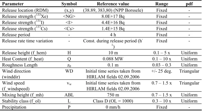
In general a uniform probability distribution function (pdf) was chosen unless additional information is available, in which case a triangular distribution was assigned. This is the case for e.g. wind speed and direction for which estimates from the meteorological expert is available at any moment. An overview of the parameter uncertainty ranges is given in Table 2 for the scenario specific and Table 3 for the non-scenario related parameters.
Table 2. Reference values and the range of variation of the PWR5 reference scenario. Values in this table represent the parameters accessible during emergency management. The pdf is the shape of the probability distribution for the parameter.
Parameter Symbol Reference value Range pdf
Release location (RDM) (x,y) (38.89, 383,80) (NPP Borssele) Fixed -
Release strength (133Xe) <NG> 8.0E+17 Bq Fixed -
Release strength (131I) <I> 4.4E+16 Bq Fixed -
Release strength (137Cs) <Cs> 1.4E+15 Bq Fixed -
Release period - 4 h Fixed -
Release rate time variation - Const. during release period (h
-1) Fixed -
Release height (f_hem) H 10 m 0.1 – 5 x Uniform
Heat Content (f_heat) Q 0.088 MW 0.1 – 10 x Uniform
Roughness Length z0 0.1 m 0.03 – 0.3 Uniform
Wind direction (winddir)
WD Initial time series taken from HIRLAM fields 02.09.2006
+/- 25 deg. Triangular Wind speed
(f_windspeed)
vw Initial time series taken from
HIRLAM fields 02.09.2006
0.7 – 1.5 x Triangular
Mixing height (f_mh) ABL 750 m 0.7 – 1.5 x Uniform
Stability class (f_ol) L Class D (OL = 1000) 0.3 – 10 x Uniform
Table 3. Standard values of model parameters in the reference scenario. Parameters reflect modelled processes included in uncertainty and parameter optimisation analyses.
Parameter Symbol Reference value Range pdf
Initial plume width (f_siginit)
σinit 0.03 km 0.3 – 10 x Uniform
Surface resistance (I) (f_rc) rc 500 s/m 0.1 – 2.0 x Uniform
Surface resistance for aerosols (Cs) (f_rc)
rc 500 s/m 0.1 – 2.0 x Uniform
Scavenging coef. mixing layer iodine (f_scav1)
ΛMixing 1.1E-5 [s-1] * 0.7 – 10.0 x Uniform.
Scavenging coef. transport layer iodine (f_scav2)
ΛTranspor t
7.0E-5 [s-1] * n.a n.a.
Scavenging coef. mixing layer (f_scav1)
ΛMixing 1.1E-5 [s-1] * 0.7 – 10 x Uniform
Scavenging coef. transport layer (f_scav2)
Λ-Transport
7.0E-5 [s-1] * n.a. n.a.
Windshear F_ws 1 0.75 – 1.25 x Tri
Cross mixing parameter crossmix 10.0 7.5 – 15.0 deg. Tri The initial plume width is related to the dimension of the source. Its range is between 10–300 m. The surface resistance parameter (rc) is used to model the dry deposition process. The 500 s/m value is
taken from the default value in the model for aerosol bounded particles (24). A large range of rc values
is reported in the literature, see e.g. (25) and references therein. The Scavenging coefficients for the mixing and transport layer are also taken from the operational model. In the case study however, precipitation processes where assumed only in the mixing layer. The use of local meteorological parameters did not allow the modelling of precipitation in the transport layer. Finally the effect of uncertainty in the parameters of the dispersion process is taken into account via the Monin-Obukhov length and wind shear parameters.
The other cases are variations of the reference case defined above. The cases differ in general in one or two important properties with the reference case. The cases are defined in Table 4 and shortly described below.
Precipitation
An average precipitation rate of 0.5 mm/h is added to the scenario. It represents moderate rain intensity, but the effect on deposition extends over the full period of the plume passage. Uncertainty in precipitation rates is normally high, and mainly reflects unknown fluctuations of the precipitation rate in a particular area during passage of the plume. The wet deposition process is modelled via the ΛMixing
parameter. Since local meteorology is used in the analyses only the wet deposition process from the mixing layer is modelled here. Uncertainty in ΛMixing and the rain intensity are linearly related. It was
Table 4: Parameter and uncertainty ranges for the cases. Only the parameter values different from the reference case are shown Case variations are calculated without variations in the release profiles, except the minimum and maximum knowledge cases.
Case Value Range pdf
Precipitation P = 0.5 mm/h (plume passage) 0.1 – 3.0 x Uniform
Stable Class EF L = 30 ABL = 200 m 0.3 – 3.0 x 0.3 – 1.3 x Uniform Uniform Unstable Class AB L = -12 ABL = 1500 m WD 0.5 – 2.0 x 0.5 – 1.5 x +/- 30 deg. Uniform Uniform Triangular Low windspeed L = 1000 ABL = 750 m vw = 0.4 m/s WD 0.3 – 3.0 x 0.3 – 3.0 x 0.5 – 3.0 x +/- 105 deg. Uniform Uniform Triangular Triangular Stack Release hem = 160 m Q = 1 MW Fixed 0.1 – 10 x - Uniform Minimum knowledge Prognosis
during threat phase
<NG> = 8.0E+17 Bq <I> = 4.4E+16 Bq <Cs> 1.4E+15 Bq H = 10 m Q = 0.088 MW z0 = 0.1 WD = <HIRLAM> vw = <HIRLAM> ABL = 750 m L = 1000 P = 0.5 mm/h 0.01 – 2.0 x(1) 0.01 – 2.0 x(1) 0.01 – 2.0 x(1) 0.1 – 4.0 x 0.1 – 100 x 0.03 – 0.3 +/- 40 deg. 0.4 – 1.6 x 0.7 – 1.5 x 0.3 x – 10x 0.1 – 3.0 x Uniform Uniform Uniform Uniform Uniform Uniform Triangular Triangular Uniform Uniform Uniform Maximum knowledge Evaluation
after controlled stack release <NG> = 8.0E+17 Bq <I> = 4.4E+16 Bq <Cs> 1.4E+15 Bq H = 10 m Q = 0.088 MW z0 = 0.1 WD = <HIRLAM> vw = <HIRLAM> ABL = 750 m L = 1000 P = 0 mm/h 0.8 – 1.2 x(1) 0.8 – 1.2 x(1) 0.8 – 1.2 x(1) 0.9 – 1.1 x 0.1 – 5 x 0.05 – 0.2 +/- 10 deg. 0.8 – 1.2 x 0.8 – 1.2 x 0.6 – 4x n.a. Uniform Uniform Uniform Uniform Uniform Uniform Tri Tri Uniform Uniform n.a. Stable
The case ”stable” represents a stable stratification of the atmosphere corresponding to a Pasquill class between E and F, which an uncertainty interval ranging from -0.5 to +0.5 class. This corresponds to a Monin-Obukhov length (L) between 100 (class E, stable) and 13.3 (class F, very stable). The boundary layer is 200 m. Stability does not change during the release and dispersion period.
1 The release rates of noble gasses, aerosols and the iodine group are not independent variables. The uncertainty analysis was
Unstable
The case ”unstable” represents an unstable stratification of the atmosphere corresponding to a Pasquill class between A and B, with uncertainty interval of ± 0.5. This corresponds to a Monin-Obukhov length (L) between -6.7 (class A, very unstable) and -25 (class B, unstable). The boundary layer is 1500 m. Stability was assumed fixed during the full release and dispersion period.
Low wind speed
This case represents situations with (very) low wind speeds. The standard HIRLAM wind vectors were modified and wind speeds were lowered to about 0.4 m/s. These conditions are accompanied by large uncertainties in the wind direction, which is expected to have considerable influence on the uncertainty analysis and data assimilation.
High Stack release
Represents a high, 160 m, release point, representing the stack height of the nuclear power plant Emsland in Germany, at 20 km from the Dutch border. The release is however not above the atmospheric boundary layer, i.e. the release is fully contained in the mixing layer of the atmosphere. The case is combined with a heat content of 1 MW.
Minimum knowledge
The minimum knowledge case describes the situation before an actual release. The accident scenario is prognosticated and estimates of release rate and meteorological conditions have large uncertainty. We have chosen to vary release rates between 0.01x and 2x of the prognosticated value. In practice larger uncertainty ranges are possible. The three release fractions, <NG>, <I> and <Cs> are assumed fully correlated, i.e. if <NG> is varied by factor “x”, the other release fractions are also varied by this factor.
Maximum knowledge
This case represents an accident scenario with maximum knowledge of the release and meteorological conditions. Determination of the release rate was possible via a stack monitoring system with an accuracy of ± 20%. Meteorological conditions are measured on-site and are therefore well known. The evaluation moment of this case is shortly after the end of the release phase. Release fractions were again assumed correlated.
2.4
Calculation endpoints and gamma station layout
Relevant endpoints for the model calculations during early phase nuclear emergency management are doses to the public and concentrations on the ground from deposition of radio nuclides. The Dutch early phase countermeasures for shelter, evacuation and iodine prophylaxis are based on an effective and a thyroid dose in the first 24 hours2 after the start of the first release phase (26). We have also
included a grazing ban, above 5000 Bq/m2 of I-131 deposition after plume passage (26) in the study. Endpoints are presented in Table 5.
2 Sheltering is sometimes evaluated using an integration period of 6 hours after the start of release. In this study we used a 24
hour period for all effective dose related endpoints to restrict the number of calculations. The effect on the uncertainty calculation is hardly influenced by this simplification since both integration periods cover the 4 hour release period.
Table 5. Calculation endpoints in the uncertainty analyses.
Calculation Endpoint Countermeasure Value Integration Period
Shelter(3) 5 mSv 24 hours (2)
Evacuation 50 mSv 24 hours
Effective dose to public
Relocation 50 mSv 1 year
Thyroid dose
(calculated for Adults)
Iodine prophylaxis for children
250 mSv(4) 24 h
Ground contamination Grazing ban 5000 Bq/m2 Plume passage
For practical reasons we have limited the effective dose (E) evaluations to 24 hour time integrated dose estimates. This conveniently covered the period of the plume passage in the evaluation area. The endpoints were not directly calculated but were constructed from the calculated time integrated air concentrations after 24 hours (TIC24) for noble gasses, the iodine-group and aerosols, respectively represented by 133Xe, 131I and 137Cs and the time integrated deposition (TID24) values from the model. From the TIC24-values effective doses can simply be deduced using a conversion factor. The same method was applied to determine an effective yearly dose estimate from the deposited 137Cs concentration. A correction value of 0.5 was applied to account for dose reductions due to the wash out of radio nuclides from the urban environment due to precipitation (27). The conversion factors applied on TIC24 for the early phase countermeasures and TID24 for the grazing ban and relocation are given in Table 6. Where appropriate the relative weight of the three nuclide groups to the effective dose (E) was taken into account in the analyses. The relative contribution to E is also given in the table. In the early phase the inhalation component dominates the dose estimate, these are easily extracted from the TIC24-values for the three nuclide groups. The year doses and the iodine contamination however is dominated by the deposition, e.g. external radiation.
Table 6. Conversion factors from TIC24 and TID24 per nuclide to a 24 hour integrated effective dose (E), thyroid dose (Ht), effective year dose estimate (Ey) and iodine contamination on the ground (CI) after plume passage.
Conversion factors are approximate numbers, assumed constant over time and space. Model Output Effective dose E mSv/Bq.h.m-3 Fraction of nuclide group to E Thyroid dose HT mSv/Bq.h.m-3 Year dose EY mSv.a-1 per Bq.h.m-2 Ground conc. CI Bq.m-2/Bq.h.m-2
TIC24 131I 24.6E-6 63% 284E-6 - -
TIC24 137 Cs 0.8E-3 21% - - -
TIC24 133Xe 1.25E-6 16% - - -
TID24 137Cs - - - 2.2E-6 -
TID24 131I - - - - 6.0E-3
The model output is calculated at several fixed locations. They are based on existing measurement locations of the NMR. The selected locations are given in Table 7 and described below:
3 Dutch intervention levels have a range of values in which health effects of countermeasures against other variables are
optimized. In this study we used low values of the intervention level for shelter and evacuation for simplicity.
1. (‘s Heerenhoek) represents the local area around the power plant and close to the centre axis of the plume. This location is represented by the NMR γ-station 1256, in ‘s Heerenhoek at 4 km from the release point.
2. (Goes) the city of Goes at a distance of 15 km, Goes has 37.000 inhabitants. An evacuation order has sizeable consequences in this area. City of Goes is in the centre plume axis and is represented by a mobile measuring station (id=2001) in the city centre.
3. (St Maartensdijk) NMR γ-station at about 30 km, it represents the practical limit of the validity of local meteorology used in the dispersion calculations.
4. (Stavenisse) NMR station 1208 also at 30 km, but at an off centre-axis position. 5. (Zuid Bijerland) NMR station 1028 at 60 km on the plume axis.
6. (Rotterdam) NMR station 1040 at 80 km on the plume axis. Rotterdam has 600.000 inhabitants and is therefore of major concern when countermeasures are to be considered.
Table 7. Locations of evaluation points of uncertainty analysis. Locations ‘s Heerenhoek, Stavenisse, Zuid Beijerland and Rotterdam coincide with a location of an NMR station. Co-ordinates are given in the system “Shifted Polar 60 deg.” (SP60). The coordinate system corresponds to the HIRLAM fields.
Location NMR Id. Distance to NPP Coordinates in SP60
‘s Heerenhoek (local area) 1256 4 km (2.37, 8.48)
Goes 2001 15 km (2.45, 8.42)
St Maartensdijk 2002 30 km (2.56, 8.34)
Stavenisse (off-axis) 1208 30 km (2.50, 8.30)
Zuid Beijerland 1028 60 km (2.73, 8.16)
Rotterdam 1040 80 km (2.87, 8,03)
In this study calculation endpoints are integrated ambient dose rates in units of H*(10) over suitable time intervals. The primary focus is on the first hour optimisation of model and release parameters. We have chosen to use hourly integrated air concentrations in the feedback loop of the optimisation method. The use of hourly updated ambient dose rates was motivated by several factors.
1. Time integrated ambient dose measurements are related to received doses to the public and thus represent an endpoint of direct interest in early phase emergency management
2. Hourly averaged ambient dose rate measurements are less sensitive to fluctuations in meteorological conditions and release quantity over time scales below the averaging period (including the exact timing of the start of release).
3. Hourly optimisations of the dispersion model require less processing time as compared to the minimum time period of ten minutes the measuring network.
Of course the method is not limited to hourly integrated measurements. At the expense of a factor of six increase in processing time the minimum averaging period can be set to the 10 minutes evaluation period of the National Measuring Network.
The data assimilation study was performed using three distinct monitoring configurations. They are shown in Figure 2(a)-(d). In (a) an equidistance grid geometry guarantees sufficient measurement locations under all conditions. The measurement locations on top of or very close to the release point are excluded, since the large dose rate values would dominate the comparison too much. In (b), a circular geometry was configured at 5 and 10 km distance. This geometry resembles the existing rings of increased density of the National Measuring Network around the nuclear power plant of Borssele. This geometry is applied several times with decreasing monitoring density; (b) and (c). Finally in (d),
the existing monitoring locations of the NMR with two additional mobile measuring stations are used to demonstrate the applicability of the method under operational conditions.
# # # # # # # # # # # # # # # # # # # # # # # # # # # # # # # # # # # # # # # # # # # # # # # # # # # # # # # # # # # # # # # # # # # # # # # # # # # # # # # # # # # # # # # # # # # # # # # # # # # # # # # # # # # # # # # # # # # # # # # # # # # # # # # # # # # # # # # # # # # # # # # # # # # ## # # ## # # ## # # # # # # # # # # # # # # # # # # # # # # # # # # # # # # # # # # # # # # # # # # # # # # # # # # # # # # # # # # # # # # # ## # ## ## ## ## ## ## # # ## # # # # # # # # # # ## # # # # # # # # # # # # # # # # # # # # # # # # # # # # # # # # ## ## ## ## # # # # # # # # # # # # # # # # # # # # # # # # # # # # 1197 1199 1201 1202 1207 1208 1212 1214 1215 1216 123 1252 1253 1254 1255 1256 1257 1258 1259 1260 1261 1262 Mob1 Mob2
Figure 2. Configurations of monitoring locations for the case study. (a) equidistance grid, (b) double circular geometry, (c) double circular geometry with reduced density, (d) the existing NMR locations and two additional mobile measurement locations (Mob1, Mob2).
(a) Grid Geometry (b) Circular Geometry (40)
3
Proof of concept
In the proof of concept the parameter optimisation method is demonstrated, based on the Kincaid data set. The selection of parameters is based on a sensitivity study of model parameters. This study differs from the case study presented in the next chapters in one important aspect: the analysis is demonstrated here on a real and well known data set, while the case study uses the model itself to generate an appropriate set of reference measurements.
3.1
Sensitivity analysis
Based on the modelled processes in NPK-PUFF, we have identified parameters contributing to the variation of the model outcome. To quantify the sensitivity of the various input parameters we applied the overall ranking number from the Model Validation Tool (MVT). The measured time-integrated concentration in air is compared with the NPK-PUFF results after varying a specific input parameter. The sensitivity analysis for the parameter describing the mixing layer height or atmospheric boundary layer (ABL) is shown in Figure 3a. The standard mixing layer height profile (in time) increased from 484 to 2274 m. This was adjusted by a multiplication factor fABL between 0.3 and 2 per model run. An
optimum was found for fABL ≈ 0.9, i.e. close to unity as expected. This demonstrates that the observed
mixing layer height profile (in time) of the Kincaid data set agrees well with our dispersion calculations when ranked using the MVT method. A sensitivity analysis of the wind direction (WD) is shown in Figure 3b. The default input wind directions were changed for all (24) model hours. It can be seen that for this particular day the registered wind direction in the Kincaid data set corresponds well with the MVT ranking results and the MVT method allows relative good determination of the daily averaged wind direction. Other parameters studied include the effective emission height (hem), the wind speed
(vw), the Monin-Obukhov length (L), the time step (dt); a model parameter describing the smallest
internal time step of the calculations, and the grid size; the dimensioning of the equidistance output grid. Results of the sensitivity analyses for these parameters are shown in Figure 3c-g. Results of MVT variability for these parameters were generally found less pronounced than those from the mixing height and wind direction. Although the effective emission height does show a minimum around the expected value of about 700 m, the MVT response is rather weak with respect to parameter changes. The same holds for the Monin-Obukhov length and the variation of the (hourly averaged) wind speed parameter. Although optimum values of the MVT function could be extracted and found in agreement to the expected values, it is likely that the daily averaged air concentrations make MVT scores of these parameters relatively independent of these parameter variations. The grid size and time step parameters represent typical examples of model implementation parameters. Both optimise at low values, i.e. smaller time steps and a smaller grid size tend to make calculations more accurate. In all further analyses optimum grid sizes (< 0.05 degree) and time step (10 minutes) were selected.
More model parameters (not shown) in the sensitivity study include the roughness length (z0), the
initial horizontal dispersion coefficient (σy) and the surface resistance (rc). Sensitivity analyses for
these parameters showed little or no variation of the corresponding MVT values. To a large degree this was anticipated. The effective release height is several hundred meters (about 700 m), which make the parameters influencing the local ground level air concentration (σy) and the deposition processes (rc, z0)
Figure 3. Sensitivity, expressed in the MVT ranking, of the day summed air concentrations of the NPK-PUFF dispersion model for (a) atmospheric boundary layer ( fABL), (b) variation in wind direction (WD), (c) emission
height (hem), (d) wind speed (wv), (e-f) the Monin-Obukhov length, for L<0 and L>0 respectively, (g) the model
time step (dt), and (h) model output grid size.
(a) Atmospheric Boundary Layer
30 40 50 60 70 80 0 0.5 1 1.5 2 f_ABL [x] M V T-ra nki n g (b) Wind Direction 30 40 50 60 70 80 -30 -10 10 30 50
Wind Direction Variation [°]
M V T-ra nk in g (c) Emission Height 30 40 50 60 70 80 0 200 400 600 800 1000 1200 1400 Emission Height [m] M V T-ra nki n g (d) Wind Speed 30 40 50 60 70 80 0 2 4 6
Wind Speed Variation [x]
MV T -r a n k in g
(f) Monin Obukov Length
30 40 50 60 70 80 1 10 100 1000 10000 MO Length [m] MV T -r an ki n g
(e) Monin Obukov Length
30 40 50 60 70 80 1 10 100 1000 10000 MO Length [m] MV T -r a n k in g --- -Neutral Stable Unstable (g) Time Step 30 40 50 60 70 80 0 0.2 0.4 0.6 0.8 1 dt [h] MV T -r a n k in g (h) Grid Size 30 40 50 60 70 80 0 0.05 0.1 0.15 0.2 Grid Size [°] M V T-ra nki n g
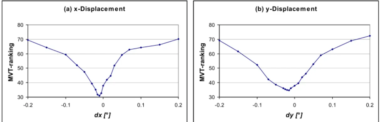
Figure 4 shows the MVT sensitivity as a function of the release location (x,y). Although the release location is normally well known when releases from nuclear power plants are concerned, unidentified releases can to some extent be localised using the techniques. The figure shows large sensitivity with respect to (small) geographical displacements. The horizontal scale spans a range from -0.2 to +0.2 degrees (in rotated latitude-longitude) which corresponds to about 44 km (North-South) and 28 km (East-West). If releases contain large heat contents the locations found in this way may deviate slightly from the real value since the effect of plume rise due to heat content may shift the (apparent) release location from the real stack location. This effect is visible in the figure.
Figure 4. Sensitivity for small displacements of the release location in (a) x- and (b) the y-direction.
3.2
Optimisations in two dimensions
In Figure 5, the results are shown of the data assimilation technique using the effective emission height and the wind vector as adjustable parameters. For both the effective emission heights and the wind vectors (measured at an altitude of 100 m) the adjustments were kept the same for all the hours at one iteration step. So, for the first iteration step, the effective emission height was kept at 400 m and the wind angle correction was kept at 0 degrees for all hours. Kincaid day July 25, 1980 was evaluated as the input data and observed data. The reason is that assumed wind vectors for this day of the Kincaid data set appeared to be inconsistent (28) with the measurements. One of the questions was if the minimisation routine was able to find a correct minimum for this particular situation. Results are shown in Figure 5 and Figure 6. The original ranking performance showed extreme disagreement. Then, after some 25 iterations the ranking parameter value dropped to 57.7, indicating a “reasonable” agreement. After 42 iterations, the minimisation procedure BCPOL stopped as the cut-off criterion was satisfied. The effective emission height was determined to be some 1070 m and the original input wind vectors were changed about 54 degrees. Validating the NPK-PUFF model in a previous instance the effective emission height was calculated to some 700 m (22). Depending on the atmospheric conditions it is of course possible that the effective emission height (or centre of mass of the puff) is in effect higher, due to an underestimated thermal plume rise of the initial stage in combination with high mixing heights (29). Other possibilities are 1. the model was unable to describe the complex physical state or 2. that an incomplete set of parameters is optimised, thereby leading to spurious data assimilation results.
In Figure 6, the results of the data assimilation are shown using a geographical information system. It is clear that the modelled results are significantly improved (final iteration). Nevertheless, the calculated dispersion is rather compact compared to the observed concentrations. Therefore, the dispersion calculation may be further improved if more input parameters (e.g., surface resistance, Monin-Obukhov
(a) x-Displacem ent
30 40 50 60 70 80 -0.2 -0.1 0 0.1 0.2 dx [°] MVT-rank in g (b) y-Displacem ent 30 40 50 60 70 80 -0.2 -0.1 0 0.1 0.2 dy [°] MVT-rank in g
length, mixing height) were used in this data assimilation. On the other hand, it is of importance that the number of iterations remains limited in order to deliver an improved prognosis in time. By identifying the most important parameters using the sensitivity and uncertainty analysis an optimisation with respect to computing time can be made.
0 20 40 60 80 100 120 0 5 10 15 20 25 30 35 40 45 iteration number MVT ranking value effective height/10 (m) wind angle correction (deg)
Figure 5. Results of the data assimilation technique applied on the two parameters, wind direction and the (effective) emission height for Kincaid day July 25, 1980 (21). Start values were 400 m emission height and zero degrees wind direction offset. Parameters progressively iterate towards their final values. The MVT ranking minimises slightly below 60. The lines are drawn to guide the eye. Results are from (7).
Figure 6. Graphical representation of the result of the fitting procedure for Kincaid day July 25, 1980. The crosses represent receptor points, the filled contours show the interpolated observed concentrations, and the other contours are the modelled results of the first (- - -) and last (——) iteration. Results are from (7).
3.3
Optimising the multi-dimensional parameter space
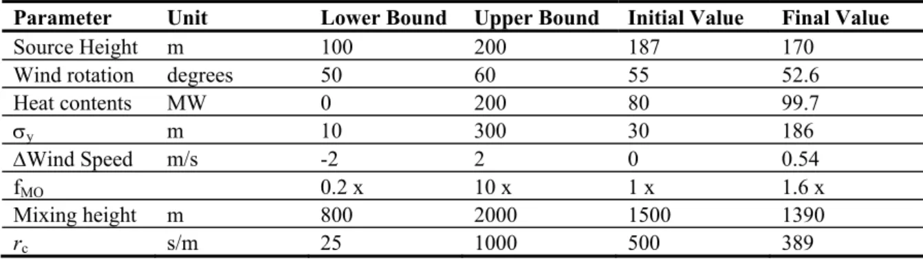
The next step was the simultaneous optimisation of eight (nine when the emission strength is also included) parameters. The model parameters are given in Table 8. Parameters were selected based on the previous sensitivity study and uncertainty analyses (30), presented in section 3.1. The initial values,
km iteration 1 final iteration -20 -10 0 10 20 30 40 km -10 0 10 20 30 40
the lower and upper bounds and the final parameter values after optimisation are given in the table. The cut-off value for the optimisation loop was set at 0,5% relative to the minimum MVT value resulting from previous iterations. The minimisation routine reached its minimum value of 40.8 after 267 iterations with eight parameters, i.e. with fixed emission strength. Inclusion of the emission strength dropped the MVT value to 39.5, comparable to the “eight parameter” optimisation run. However, as the cut off criterion was reached much sooner after about 125 iterations, the algorithm was much faster then in the eight-parameter optimisation run. The MVT values indicate a “reasonable” agreement between predicted and observed data.
Table 8. Initial and final parameter values of the model optimisation run.
Parameter Unit Lower Bound Upper Bound Initial Value Final Value
Source Height m 100 200 187 170
Wind rotation degrees 50 60 55 52.6
Heat contents MW 0 200 80 99.7 σy m 10 300 30 186 ΔWind Speed m/s -2 2 0 0.54 fMO 0.2 x 10 x 1 x 1.6 x Mixing height m 800 2000 1500 1390 rc s/m 25 1000 500 389
Figure 7 shows the MVT values per iteration for the optimisation runs. In Figure 8 the graphical representation of the modelled daily time-integrated air concentration is shown. Compared to the two parameter optimization from the previous section the improvement is visible and is further reflected in the lower MVT ranking number after optimisation. The results from Table 8 show that final parameter values are found that are in conceivable range of the expected values.
0 20 40 60 80 100 0 50 100 150 200 250 number iterations M V T rank 8 parameters 9 parameters
Figure 7. The number of iterations and the MVT ranking value per iteration step for the 8 and 9 parameter optimisation runs with the NPK-PUFF model.
The results of the NPK-PUFF optimisation for the full Kincaid data set5, can be compared to the results
without the parameter optimisations. Figure 9 shows the results of this comparison as a function of the
5 The TSTEP and WinREM models use only 19 and 21 Kincaid data days respectively. In the remaining days the release
conditions were unfavorable for the respective models, e.g., a substantial part of the release went directly into the reservoir layer.
daily averaged air concentration for all Kincaid days. If data assimilation is turned on the final MVT ranking after optimisation id reduced between 10 – 50 points, indicating better agreement between modelled output and measurements.
Figure 8. Graphical representation of the modeled output for the first and the final iteration.
Figure 9. Overview of MVT ranking numbers for the daily integrated air concentration per Kincaid day for the NPK-PUFF dispersion model, with and without the data assimilation.
The results in this chapter clearly show the potential improvements in modelled time-integrated air concentrations that can be obtained by applying the parameter optimisation method. These results demonstrate a proof of concept of the methodology and further investigations into the applicability seems appropriate. This will be the topic of chapter 5, after we investigate the effect of parameter uncertainty in the model (chapter 4).
0 20 40 60 80 100 0 5 10 15 20 25
Kincaid day number
NPK-PUFF MVT MVT rank iteration 1 final iteration -20 -10 0 10 20 30 40 km -10 0 10 20 30 40 km
4
Case study uncertainty
In this chapter we investigate the combined effect of input parameter uncertainty on the model output. The simulated cases, defined in chapter 2 are used in this analysis. The identification of relevant parameters followed from the sensitivity study of chapter 3. The range of model input parameters is used in the model calculations to determine a range of model output values. We will use the range of model output values as an indicator for the model uncertainty. At the end of this chapter the input model parameters are ranked with respect to their contribution to the overall model output uncertainty. This ranking provides the basis for parameter selection for the data assimilation technique of chapter 5. In the uncertainty analysis, we analyse and present modelled results of the following observables at the monitoring locations.
1. The uncertainty factor (UF, UF*) of the model output
2. Probability of finding doses above the sheltering and evacuation threshold (5 and 50 mSv) 3. Probability of finding a grazing ban (5000 Bq/m3 of 131I)
4. Probability of finding a year dose above the intervention for relocation (50 mSv/year) 5. Probability of finding a thyroid dose above 500 mSv for children (=250 mSv for adults) The uncertainty factor (UF) is defined as the ratio of the 95% over 5% output values of the cumulative and normalized subjective probability function P(Y ≤ y), defined in section 2.2. We will use this ratio as a measure of uncertainty for a certain endpoint, usually a dose, received over a certain time period. In some cases the value of the probability function at y=0 (model output has value zero) can be larger than zero, i.e. the model calculates doses of zero value in a number of instances at a particular location. In other words not all variations of the radioactive plume reach the evaluation location. In these cases a corrected UF* value is defined as the ratio of 95% to 5% values, excluding the model outputs of value zero.
4.1
Standard model output for the reference case
An example of the model output based on the reference scenario is shown in Figure 10. Shown are the air concentration of 131I after 2, 4, 6 and 8 hours, the 131I concentration on the ground after plume passage and the effective dose to the public, 24 hours after the start of the release. The radioactive cloud is following the prevailing south-south-west wind direction and threatens several communities, e.g. Goes at 15 km and the city of Rotterdam at about 70-80 km distance. The calculations are performed using standard parameter values from Table 2 and Table 3. From the model output it can be seen that the intervention level for sheltering (5 mSv/24h) is exceeded to almost the city of Goes, at 15 km distances. Iodine prophylaxis for children is exceeded up to distances of almost 5 km. A grazing ban is exceeded in the full evaluation area.
4.2
Reference case
The uncertainty analysis for the reference case was based on the parameters from Table 2 and Table 3. Figure 11 shows the results. Source strength variations are not included here. The figure shows
subjective probabilities P(Y>y), i.e., (1 - P(Y≤y)), of finding model values Y above the value y. The horizontal scale (y) of the figure shows time-integrated concentration or deposition and is converted into the appropriate endpoint: effective dose, thyroid dose, yearly received dose from external radiation using the conversion factors from Table 6 in section 2.4.
Figure 10. Footprints from the reference PWR5 release showing 131I air concentration at (a) t=2, (b) t=4, (c) t=6
hours, and (d) t=8 hours; (e) 131I concentration on the ground from (dry) deposition after cloud passage and (f)
the calculated effective dose, E after 24 hours. Dutch intervention levels for shelter and evacuation are at 5 and 50 mSv respectively (low levels).
Table 9. The effective dose reference value, the 5% and 95% values and the uncertainty factor (UF) for the reference case without variations in the source strength.
Reference value (mSv) 5% (mSv) 95% (mSv) Uncertainty factor (UF) ‘s Heerenhoek (4 km) 43.3 14.2 65.5 4.6 Goes (15 km) 11.8 4.3 16.1 3.7 St Maartensdijk (30 km) 5.6 1.4 7.9 5.6 Stavenisse (30 km, off-axis) 2.4 0.6 6.5 11.3 Zuid Beijerland (60 km) 2.7 0.8 3.8 5.1 Rotterdam (80 km) 1.9 0.4 2.7 6.8
Uncertainty factors range from 3.7 in Goes to 11.3 in Stavenisse. Stavenisse represents an off-axis location, i.e. at the very outside of the cloud coverage in that area. On these locations variations in e.g. wind direction is expected to have there largest influence on the model outcomes and therefore the uncertainty estimates. It is further seen that the uncertainty increases with the travelling distance of the radioactive cloud. The reference model output is usually centred in the middle of the cdf curve. This could be expected, since the uncertainty range on the individual parameters is also centred around these “best estimates”. (a) Concentration in Air t+2 h (b) Concentration in Air t+4 h (c) Concentration in Air t+6 h (d) Concentration in Air t+8 h (e) I-131 Ground Contamination kBq/m2 (f) Effective Dose (mSv) t+24 h
(a) Effective Dose (24 h) 1028 1040 1208 1256 2001 2002 0 0.1 0.2 0.3 0.4 0.5 0.6 0.7 0.8 0.9 1 0.1 1 10 100 1000 E (mSv) P ro ba bil ity P (Y > y) 1256 4 km 's Heerenhoek 2001 15 km Goes 2002 30 km St Maartensdijk 1208 30 km Stavenisse 1028 60 km Zuid Beijerland 1040 80 km Rotterdam
(b) Thyroid Dose Adults (24h)
1028 1040 1208 1256 2001 2002 0 0.1 0.2 0.3 0.4 0.5 0.6 0.7 0.8 0.9 1 1 10 100 1000 10000 Thyroid Dose (mSv) P ro ba bi lity P (Y > y) 1256 4 km 's Heerenhoek 2001 15 km Goes 2002 30 km St Maartensdijk 1208 30 km Stavenisse 1028 60 km Zuid Beijerland 1040 80 km Rotterdam
(c) Year Dose from Deposition
1028 1040 1208 1256 2001 2002 0 0.1 0.2 0.3 0.4 0.5 0.6 0.7 0.8 0.9 1 0.01 0.1 1 10 100
First year effective dose (mSv)
P ro ba bilit y P (Y > y) 1256 4 km 's Heerenhoek 2001 15 km Goes 2002 30 km St Maartensdijk 1208 30 km Stavenisse 1028 60 km Zuid Beijerland 1040 80 km Rotterdam
Figure 11. Subjective probability distributions for (a) effective dose P(E>e), (b) thyroid dose to adults P(H>h) and (c) yearly effective dose from external radiation following deposition P(E>e). P(E>e) is the probability of finding a dose value at the indicated evaluation locations above a given value, e. Calculations are for the reference scenario without variations in the release strength. Intervention levels are 5, 50 mSv effective dose for sheltering and evacuation, 250 mSv thyroid dose for iodine prophylaxis for children and 50 mSv effective year dose for relocation.
From the data in Figure 11 confidence levels are deduced for exceeding intervention levels for effective dose, thyroid dose, a year dose from external radiation (relocation) and the grazing ban. Results are presented in Table 10.
Table 10. Subjective probabilities of exceeding intervention levels for shelter, evacuation (lower limits), iodine prophylaxis, relocation and grazing ban. Calculations based on the reference run without variations (uncertainty) in source strength.
P(E> 5 mSv) P(E> 50 mSv) P(Ht> 1000 mSv) (adults) P(Ht> 250 mSv) (children) P(E>50 mSv) (after plume passage) P(C>5000Bq/m2) ‘s Heerenhoek (4 km) (representing local area)
99.9% 13% 70%(child) 1.5% (adults) - 100% Goes (15 km) 90% - 1% (child) - 100% St Maartensdijk (30 km) 26% - - - 99% Stavenisse (30 km, off-axis) 12% - - - 98% Zuid Beijerland (60 km) 1% - - - 99% Rotterdam (80 km) - - - - 97%
From the reference model it was concluded that the intervention level for sheltering at 5 mSv was exceeded up to distances of about 15 km. From the table it is concluded that the intervention level for sheltering can be exceeded up to distances of about 30 km (and more) with significant probabilities. Evacuation at 50 mSv still has a confidence level of 13% in the local area around the release location (4 km). In the reference model output the effective dose was never above the evacuation threshold. It is clear that the introduction of uncertainty in the analysis converts statements regarding intervention levels into confidence levels of exceeding a particular intervention level. At what level, i.e. how certain one must be in order to effectuate countermeasures is beyond the scope of this case study.
4.3
Case variations
Results of the uncertainty analysis for the case variations are presented in Table 11. The reference scenario is, again, included in the table for convenience. Instead of UF, the uncertainty factors are reported in units of UF*, i.e. zero model output values are excluded when calculating the 95% over 5% ratios. If defined the uncorrected UF factors are indicated between parentheses.
In general the behaviour of the uncertainty factors compare rather well to those of the reference case. It is shown that precipitation and the stack release do not influence the uncertainty factors in the model output very much when compared to the reference case. This behaviour is expected since the 24 hour dose calculation is primarily related to the time integrated air concentration, considered in this analysis. If deposition would have been considered also, precipitation is expected to add to the overall uncertainty of the model output.
Notable differences are visible in the other cases: stable and unstable conditions increase the model output uncertainty with a factor between 2 and 5 times, compared to the reference case and up to 10 times for off-the-plume-axis (Stavenisse) locations. Uncertainty for the low wind speed scenario
also increases uncertainty, especially at larger distances: up to 2-4 times below 30 km and up to about 25 times for distances above 30 km.
Table 11. Corrected uncertainty factors, UF*, for all cases as deduced from the uncertainty analysis. The uncorrected uncertainty factors (UF) are given between parentheses if different from the UF* values. Values are deduced from the 24 hours effective dose model output.
Reference Precipitat
ion
Stable Unstable Low wind Stack ‘s Heerenhoek (4 km) 4.6 4.6 6.6 6.4 9.1 (∞) 4.2 Goes (15 km) 3.7 4.3 9.2 (11.9) 9.9 (11.4) 15.4 (∞) 4.0 St Maartensdijk (30 km) 5.6 6.3 (6.4) 21.8 (116) 12.0 (29.1) 19.4 (∞) 5.7 Stavenisse (30km, off-axis) 11.3 11.7 122 (∞) 30.1 (32.2) 20.8 (∞) 12.7 Zuid Beijerland (60 km) 5.0 (5.1) 6.9 17 (68) 12.9 (24.9) 129 (∞) 4.9 Rotterdam (80 km) 6.1 (6.8) 8.4 19.9 (∞) 28.1 (83) 150 (∞) 6.5
4.4
Cases with minimum and maximum knowledge
In operational emergency management situations, uncertainty of the model parameters can be considerably larger then presented in the cases above. The case “minimum knowledge” represents such a scenario. Here, little is known a priori about the release strength, the release conditions and the meteorology. In practice, the minimum knowledge case represents conditions before the actual release takes place. The primary objective of these calculations is the evaluation of early countermeasures and so, uncertainty in the release strength is explicitly included in the analysis. The reference parameter values in the minimum knowledge case are chosen such that the release quantity is estimated conservative, i.e. the uncertainty range extents more towards the lower parameter values (uncertainty in release strength is in range 0.01 – 2x). The case “maximum knowledge” represents a scenario with relatively good knowledge of the release quantity and other case parameters. One can think of the maximum case as being constructed shortly after the release has occurred and the dominating nuclide compositions (Noble gasses, Iodine and aerosols) could accurately (±20%) be determined by a stack monitoring system. Table 12 to table 15 give results on uncertainty factors and intervention levels. The variation of release strength in the analyses was assumed correlated, i..e, if the fraction of noble gasses was varied a factor y, the aerosols (Cs) and iodine (I) groups release rates were also varied with this factor y. This correlation is conceivable in reality. Here it maximises the uncertainty fraction, UF or UF*.
Table 12. Case maximum knowledge. Reference value, 5% and 95% percentiles of 24 hours effective dose, and the corrected uncertainty factors.
Reference value (mSv) 5% (mSv) 95% (mSv) Uncertainty factor UF* (UF) ‘s Heerenhoek (4 km) 27.5 12.7 43 3.4(3.4) Goes (15 km) 7 4.2 10 2.5 (2.5) St Maartensdijk (30 km) 3.4 2.1 5 2.4 (2.4) Stavenisse (30 km, off-axis) 1.5 0.3 3 8.9 (8.9) Zuid Beijerland (60 km) 1.6 1.0 2 2.4 (2.4) Rotterdam (80 km) 1.1 0.7 1.7 2.4 (2.4)
Table 13. Case with minimum knowledge. Reference value, 5% and 95% percentiles of 24 hours effective dose, and the corrected uncertainty factors.
Reference value (mSv) 5% (mSv) 95% (mSv) Uncertainty factor UF* (UF) ‘s Heerenhoek (4 km) 27.5 1.90 51 27.4 (51) Goes (15 km) 7 0.1 13 37.7 (94.5) St Maartensdijk (30 km) 3.4 0 6 54.5 (∞) Stavenisse (30 km, off-axis) 1.5 0.09 4.7 48 (51) Zuid Beijerland (60 km) 1.6 0.01 3 50.0 (540) Rotterdam (80 km) 1.1 0 2 49.1 (∞)
Table 14. Case with maximum knowledge. Subjective probabilities of exceeding intervention levels for shelter, evacuation, iodine prophylaxis, relocation and the grazing ban.
P(E> 5 mSv) P(E> 50 mSv) P(Ht> 1000 (250) mSv) (adults/child) P(E>50 mSv) (after plume passage) P(C>5000 Bq/m2) ‘s Heerenhoek (4 km) 100% 1% 0.05% (adults) 93% (child) 0.1% 100% Goes (15 km) 88% - - - 100% St Maartensdijk (30 km) 5% - - - 100% Stavenisse (30 km, off-axis) - - - - 100% Zuid Beijerland (60 km) - - - - 100% Rotterdam (80 km) - - - - 100%
Table 15. Case with minimum knowledge. Subjective probabilities of exceeding intervention levels for shelter, evacuation, iodine prophylaxis, relocation and the grazing ban.
P(E> 5 mSv) P(E> 50 mSv) P(Ht> 1000 (250) mSv) (adults/child) P(E>50 mSv) (after plume passage) P(C>5000 Bq/m2) ‘s Heerenhoek (4 km) 82% 5% 5% (adults) 50% (child) 34% 99% Goes (15 km) 43% - 4% 7% 94% St Maartensdijk (30 km) 8% - - 0.4% 85% Stavenisse (30 km, off-axis) 5% - - - 87% Zuid Beijerland (60 km) 1% - - - 75% Rotterdam (80 km) - - - - 65%