Multiple stress by repeated use
of plant protection products in
agricultural areas
Colophon
© RIVM 2017
Parts of this publication may be reproduced, provided acknowledgement is given to: National Institute for Public Health and the Environment, along with the title and year of publication.
R. Luttik (author), RIVM (retired in 2013)
M.I. Zorn (author), College voor de toelating van gewasbeschermingsmiddelen en biociden
T.C.M. Brock (author), Wageningen Environmental Research E.W.M. Roex (author), Deltares
A.M.A. van der Linden (author), RIVM Contact:
Ton van der Linden
ton.van.der.linden@rivm.nl
This investigation has been performed by order and for the account of the Ministry of Infrastructure and the Environment, within the
framework of the project Risk Assessment Methodology (RIVM) and the framework of the project KPP fresh water quality (Deltares) and the Ministry of Economic Affairs, within the framework of project BO-AGRO M&G-BTG-001 Instruments for risk assessment of aquatic organisms.
This is a publication of:
National Institute for Public Health and the Environment
Synopsis
Multiple stress by repeated use of plant protection products in agricultural areas
Current risk assessment of plant protection products is performed on a formulated-product-by-formulated-product basis and does not take into account the fact that products may be mixed and/or that different products are used sequentially within a growing season. This report evaluates three possibilities for taking these aspects into account in the future that target the risks for surface water. The investigated methods have been shown to be able to take ‘multiple stresses’ into consideration. Further investigation is needed to check if these methods are sufficient.
In this report, three different methods were used to assess the multiple stresses caused by parallel and sequential applications of plant protection products according to realistic application scenarios during the growing season of a tuber crop and an orchard crop. The methods show the effects of the different products on the organisms living in a ditch at the edge of a field. The first method used is the so-called Toxic Unit method, in which the contributions of the individual substances to the overall toxicity are summed and the maximum in time is calculated. The second method, the mixture toxic pressure method (msPAF), calculates the potentially affected fraction of aquatic organisms, taking into account differences in the sensitivity of the organisms to the various substances. The third method, the MASTEP population model, calculates the time necessary for a sensitive aquatic organism (an aquatic isopod) to recover from its exposure to the various substances. The Toxic Unit method (TU) is the one most comparable to the current authorization assessment.
All three methods show that a few substances determine a large part of the calculated total effect. The TU-method and the mixture toxic pressure (msPAF) method are useful in identifying these active substances. These selected substances were then used in the MASTEP calculations. The MASTEP method, using Asellus aquaticus as indicator species, did indicate no or hardly any longer recovery times for the multiple applications in comparison with those calculated for the individual pesticide applications. This result applies to species with a high number of offspring. It is recommended that the MASTEP method is used with water organisms that have other survival strategies.
At the moment, EFSA (European Food Safety Authority) undertakes activities to develop tools and guidance to assess the human and ecological risks of combined exposure to multiple active substances. This report can contribute to these activities.
Keywords: plant protection products, environmental risk assessment, tank mixture, sequential applications, surface water, multiple stresses, recovery, Toxic Unit (TU), mixture toxic pressure (msPAF), MASTEP
Publiekssamenvatting
Meervoudige stress door herhaaldelijk gebruik van gewasbeschermingsmiddelen in landbouwgebieden
In de huidige toelatingsbeoordeling van gewasbeschermingsmiddelen worden effecten beoordeeld op basis van de werkzame stoffen die er in zitten. Er wordt daarbij geen rekening mee gehouden dat er meerdere
gewasbeschermingsmiddelen, met andere werkzame stoffen, bij dezelfde teelt worden gebruikt. Dit onderzoek verkent drie mogelijkheden om hier in de toekomst wel rekening mee te houden, gericht op de risico’s voor
oppervlaktewater. De onderzochte methoden blijken deze ‘meervoudige stress’ te kunnen meenemen. Wel is meer onderzoek nodig om na te gaan of deze methoden toereikend zijn.
Voor dit onderzoek zijn met de drie methoden realistische scenario’s van het gebruik van gewasbeschermingsmiddelen binnen een groeiseizoen voor een knolgewas en een fruitteeltgewas doorgerekend. De methoden nemen de effecten mee die de verschillende middelen hebben op de organismen in de nabijgelegen sloot. Een van de methoden telt toxiciteitsindexen bij elkaar op (de Toxic Unit-methode, TU), een andere houdt rekening met verschillen in gevoeligheid van soorten organismen voor het bestrijdingsmiddel (de toxisch druk-methode, msPAF) en de derde methode berekent effecten op en het herstel van een gevoelig waterorganisme (het MASTEP-populatiemodel voor de waterpissebed). De TU-methode is het meest vergelijkbaar met de huidige toelatingsbeoordeling.
Bij alle drie de methoden blijkt dat enkele stoffen een groot deel van het totaal berekende effect bepalen. De TU-methode en de toxische druk-methode (msPAF) blijken nuttig om deze werkzame stoffen te bepalen. Met deze werkzame stoffen zijn vervolgens de MASTEP-berekeningen uitgevoerd. Uit de MASTEP-berekeningen blijkt dat de periode die de waterpissebed nodig heeft om te herstellen van het effect van de middelen niet of
nauwelijks langer duurt als meerdere middelen tegelijk worden gebruikt. Dit resultaat geldt voor waterorganismen die als overlevingsstrategie hebben dat ze veel nakomelingen produceren. Het verdient aanbeveling de MASTEP-berekeningen ook uit te voeren voor organismen met andere
overlevingsstrategieën.
EFSA (European Food Safety Authority) zoekt momenteel naar
mogelijkheden om richtlijnen en instrumenten te ontwikkelen voor het beoordelen van de risico’s van gecombineerde blootstelling van mens en milieu aan meerdere werkzame stoffen. Dit rapport kan hieraan bijdragen. Kernwoorden: gewasbeschermingsmiddelen, milieurisicobeoordeling, oppervlaktewater, tankmengsel, meervoudige stress, herstel, Toxic Unit (TU), toxische druk (msPAF), MASTEP
Contents
Summary — 9
1 Introduction — 11
2 The use of tank mixtures in agriculture — 13
2.1 Introduction — 13 2.2 Tank mixing — 13
3 Realistic worst-case crop scenarios — 15
3.1 Introduction — 15
3.2 Information on the use and environmental impact of PPP — 15 3.3 Development of realistic worst-case scenarios — 17
3.4 Results — 18
4 Impact of multiple stresses on the aquatic ecosystem — 21
4.1 Exposure assessment — 21 4.1.1 Tuber scenario — 21
4.1.2 Orchard scenario — 23 4.2 Impact assessment — 26 4.2.1 Toxic Unit (TU) approach — 27
4.2.2 Mixture toxic pressure (msPAF) approach — 27 4.2.3 The MASTEP population model — 30
4.3 Results — 32
4.3.1 Toxic Unit (TU) approach — 32
4.3.2 Mixture toxic pressure (msPAF) approach — 37 4.3.3 MASTEP calculations — 38
5 Discussion — 41
6 Conclusions and recommendations — 45
References — 47
Glossary and abbreviations — 51 Acknowledgement — 53
Appendix A Example of open field, soft fruit PPP treatment — 55 Appendix B Crops and PPP use information — 57
Appendix C Typical application regimes — 59 Appendix D Summary of an outdoor aquatic mesocosm study — 68
Summary
The environmental risk assessment of the agricultural use of plant protection products is based on the evaluation of individual substances or formulations containing a few active substances. However, plant protection schemes for a cropping period include several formulations, which may sometimes be applied in tank mixtures. Consequently, organisms in edge-of-field surface waters may become repeatedly exposed, simultaneously or consecutively, to different substances in one growing season.
This report evaluates the potential impact on aquatic ecosystems in field ditches resulting from exposure to the total plant protection product package used in representative tuber and orchard crops in the Netherlands. Three methods are used to assess these high input crops:
• the Toxic Unit approach;
• the mixture toxic pressure (msPAF)approach, and; • the MASTEP population model approach.
In the Toxic Unit approach applied here, acute toxicity estimates for the base set organisms (primary producers, crustaceans and fish) for the different products that contribute to simultaneous exposure are combined using the Concentration Addition (CA) principle.
The mixture toxic pressure approach is based on species sensitivity
distributions (SSD) for appropriate groups of organisms. SSDs are used to calculate the concentration x at which a specified proportion of species is expected to suffer from direct toxic effects, called the hazardous
concentration (HC). In this report, the SSD approach is used, based on LC50 data, in a reciprocal way and the fraction of the species that is potentially affected by the exposure to multiple substances is calculated. This fraction is indicated as the ‘multi substances Potentially Affected Fraction’ (msPAF). The MASTEP population model approach is a completely different method. In this case, the MASTEP population model developed for the aquatic isopod Asellus aquaticus is used for calculating the magnitude of effects and the time necessary for the population to recover when exposed to a sequence of plant protection products. In the population model, recovery is based on internal recovery in the stretch of ditch that is exposed to the plant
protection products, as well as on immigration from non-exposed stretches of ditch outside the treated area.
The MASTEP population model indicated cumulative effects for the orchard cases, but in both crops the simultaneous and/or repeated exposure to plant protection products hardly increased the time needed for recovery by Asellus aquaticus. It is recommended that multiple stresses for organisms with other survival strategies be investigated before drawing conclusions about current risk assessment procedures.
1
Introduction
The risk assessment of plant protection products (PPP) in the prospective legislative authorization process is based on the separate evaluation of individual active substances1 or formulated products2. Usually, a tiered
approach is followed in which the modelled concentrations of substances in an “edge-of-field ditch” are compared to the regulatory acceptable concentrations (RACs) of the substances under consideration in environmental
compartments. In the first tier, the RAC is based on threshold levels of effects, whereas in higher tiers the risk analysis may also consider the potential for ecological recovery.
The implementation of the threshold and recovery options in the aquatic risk assessment for individual substances or formulated products may be
unrealistic if different PPP are applied simultaneously, consecutively and/or repeatedly during the growing season. This multiple stress problem is also noted in an EFSA (European Food Safety Authority) opinion on the
development of specific protection goals for the environmental risk assessment of PPP (EFSA 2010).
The EFSA website3 states (December 2016):
‘People, animals and the environment can be exposed to multiple chemicals from a variety of sources. EFSA has already developed some approaches for assessing combined exposure to multiple pesticides and contaminants in humans and multiple pesticides in bees. Our scientists are developing new approaches and tools for harmonizing how we assess the risks to humans and the environment from multiple chemicals in the food chain: “chemical
mixtures” and their “cocktail effects”.
EFSA’s Scientific Committee has set up a working group of experts to develop guidance on the combined exposure to multiple chemicals. This initiative is called MixTox.’
EFSA is currently undertaking activities to contribute to the development of tools for assessing the human and ecological risks posed by single and multiple chemicals. The plan is to finalize ‘Technical reports on tiered
approaches for human and ecological risk assessment of combined exposure to multiple chemicals’ in 2017. This report can contribute to the desired tools and guidance development for mixture assessments of PPP.
1 Active substance means any substance or micro-organism, including a virus, having a general or specific action
against harmful organisms or on plants, parts of plants or plant products, or substances used to protect plants and increase their resistance to pathogens or to regulate the growth of plants.
2 Formulated product means a mixture or solution composed of two or more substances, at least one of which is an
active substance, and is intended for use as a plant protection product.
The aim of this report is to investigate the possible influences of exposure to substances resulting from realistic PPP-application regimes that currently are not considered in the authorization procedures by addressing the following questions:
1. To what extent are substances used in single tank mixtures? (See Chapter 2).
2. What are typical and realistic worst-case application scenarios for some of the important crops in the Netherlands? (See Chapter 3). 3. What is the potential impact on aquatic organisms of simultaneous,
consecutive and/or repeated application (multiple stresses) of PPP in two representative crops? (See Chapter 4).
4. What is the potential impact of these multiple stresses on the recovery of aquatic organisms? (See Chapter 4, Section 4.2.3). Two example crops are evaluated in this report as an illustration of the potential consequences of multiple exposures, but it was not the intention to be exhaustive, such that the evaluations represent a complete and final risk assessment for these crops. Data selection and scenarios used for the calculations are not necessarily in agreement with current procedures in the authorization process. Therefore, no conclusions can be drawn about the current regulatory status of the substances. Also, not all possible mitigation options were implemented or used in the scenario calculations and, besides endpoints for the substances available in the dossiers, additional toxicity values were used (see Section 4.1).
This report also does not provide a complete recipe for assessing recovery, as recovery has only been addressed using one particular model (the MASTEP population model), while other approaches exist as well. The research thus intends to demonstrate the potential relevance of multiple stresses under realistic use conditions by using several additional exposure and effect assessments.
In this report, the term ‘multiple stresses’ is related only to the effects caused by simultaneous, consecutive and / or repeated applications of PPP to a crop in one growing season. Stress due to others factors, such as temperature and drought, are not considered.
2
The use of tank mixtures in agriculture
2.1 Introduction
In the environmental risk assessment of PPP, normally applications of individual active ingredients or formulated products are taken into account, including repeated applications according to label instructions. When the formulated product contains more than one active substance, toxicity tests with the formulated product have to be made available for the dossier. In such cases, it is possible to compare the outcomes and to assess whether the substances in the formulated product behave in a synergistic or
antagonistic way. However, this is often only done for the species found to be most sensitive to the individual substances.
When a substance or formulated product is applied more than once during the growing season, the series of applications is taken into account in the authorization process. Usually this is done by accounting for the specified maximum number of applications and the minimum time interval between the applications. Yet it is common practice to apply multiple products together in so-called tank mixes (see below) and these are usually not considered in the authorization process. Only when the label specifies that a formulated product is to be used in a tank mix, is the overall toxicity of the tank mix calculated using the concept of Concentration Addition (CA); the tank mix as such is never tested. Note that in the tank mix not only can different active substances be mixed, but also additives, such as stickers and synergists, which will supposedly enhance the performance of the mixture, but may also influence unintended effects.
2.2 Tank mixing
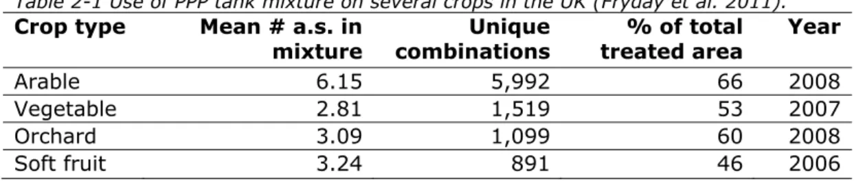
One of the few studies focused on the contents of tank mixes was published by Fryday et al. (2011). The results of this study are summarized for four different crop categories in the UK (i.e. arable crops, vegetable crops, orchards and soft fruit) in Table 2-1.
Table 2-1 Use of PPP tank mixture on several crops in the UK (Fryday et al. 2011).
Crop type Mean # a.s. in
mixture combinationsUnique treated area % of total Year
Arable 6.15 5,992 66 2008
Vegetable 2.81 1,519 53 2007
Orchard 3.09 1,099 60 2008
Soft fruit 3.24 891 46 2006
Table 2-1 shows that 66% of the arable crop area in the UK was treated in 2008 with tank mixtures and that, on average, 6.15 active substances were used per application. On 34% of the arable crop area, single formulated products were used. The table also shows that a huge variety in tank mixtures exists, as nearly 6,000 different tank mixtures were noted for the arable crops. For the other three crop categories, approximately 50% of the area was treated with tank mixtures and, on average, with three different substances per application.
These data show that the use of tank mixes in agriculture in the UK is a common phenomenon. There are no indications that this phenomenon does not occur in other member states of the European Union.
3
Realistic worst-case crop scenarios
3.1 Introduction
The purpose of this chapter is to gain insight into the package of PPP applied to particular crops during one growing season in the Netherlands, the
frequency of the applications and, to some extent, the variability in the application regimes. The aim is to present information for larger crops (in terms of crop area) in particular. The following criteria were used to obtain typical and realistic worst-case scenarios (analyses performed by the research institute “Praktijkonderzoek Plant en Omgeving” (PPO)):
1. The total amount (kg) of active substances used per hectare on a certain crop in a growing season, based on surveys by Statistics Netherlands (CBS).
2. The different categories of PPP applied to the crop (i.e. fungicides, growth regulators, herbicides, insecticides and others).
3. The number of environmental indicator points (EIPs) calculated by the Dutch Environmental Indicator (DEI; see below) for the aquatic ecosystem, for the acute situation, as well as for the chronic
situation.
4. Whether ecotoxicological studies are available for a particular crop in which the effects of multiple use of PPP in a growing season were studied.
Based on the information described in this chapter, a tuber crop and an orchard crop were selected for further investigation of the multiple stresses (Chapter 4).
3.2 Information on the use and environmental impact of PPP
The use of PPP in larger crops is described in the Dutch Environmental Indicator (Kruijne et al. 2011a, Kruijne et al. 2011b). The point of departure of the DEI is the average application rate of a substance in a crop, based on surveys conducted by CBS. Figures were adapted by 1) rounding the
application frequency to the nearest integer while keeping the total amount used on the crop and 2) accounting for non-response. An example of the underlying information for an open field soft fruit cultivation is presented in Appendix A. Appendix B gives the crops that are included in the DEI,
together with the total amounts (kg) of active ingredients of PPP used on the crop, the crop acreage and whether it is a covered crop or not. The crops in which more than 10 kg of active substance per hectare per year is applied are summarized in Table 3-1. Many of the substances in the inventory of 2004 are still on the market and plant protection management schemes have not changed dramatically (see Spruijt et al. 2011).
Table 3-1 Active substances per hectare per crop for the year 2004 for different substance classes (source DEI). All crops are field crops.
Crop
kg/ha
fungicide herbicide insecticide other fumigant total
lilies 29.8 10.4 81.5 0 11.9 133.6 pears 20.8 2.4 11.3 0 34.5 hyacinths 6.0 8.4 0 0.1 15.6 30.1 apples 20.0 2.8 2.3 0.3 25.4 irises 13.4 4.5 0.5 6.3 24.7 tulips 11.7 6.1 0.7 0.1 5.8 24.4
other fruit trees 15.3 6.2 0.9 0 22.4
gladiola 12.6 4.1 1.5 0.3 3.5 22.0 seed onions 16.1 2.9 0 1.5 20.5 narcissus 4.1 4.5 0 11.3 19.9 onions 15.3 3.2 0.6 0.1 19.2 seed potatoes 7.6 2.1 4.0 0.3 0 14.0 public green
(trees & shrubs) 1.5 2.2 0.1 0 9.6 13.4
industrial potatoes 11.2 0.9 0.1 0.8 13.0 consumption potatoes 8.2 2.4 0.2 0.3 11.1 rose shrubs 8.6 1.7 0.4 0.1 0 10.8 strawberries 8.5 1.5 0.2 0 10.2
The crops with the highest amount of PPP used per hectare are bulb species (lilies, tulips, irises and hyacinths) and fruit trees (apple, pear and other fruit trees). The crop with the highest amounts of fungicides, as well as
insecticides and herbicides, is lilies (field crop). Pear crops are characterized by the large use of fungicides and insecticides. Apple crops are characterized by the large use of fungicides, ‘other fruit trees’ and hyacinths by the large use of herbicides.
The DEI combines the use information of individual substances (for example, dose, application method and timing) with information on emission pathways (for example, drift and drainage). Next, it calculates exposure
concentrations in receiving environmental compartments and finally compares these with ecotoxicological effect concentrations. Results are expressed as Environmental Indicator Points (EIPs), which express the risk per unit area of agricultural land on which the substance is used. Results can subsequently be aggregated over crop, time and / or spatial scale to obtain appropriate risk indicators.
Table 3-2 presents the aggregated EIPs for 2004 in descending order for crops with 10 or more EIPs per hectare. For field crops, EIPs are given for both the acute and the chronic situation. For covered crops, EIPs refer only to the acute situation. Differences in the order of the EIPs are mainly due to the fact that ecotoxicological reference values differ between the acute and chronic assessment.
Table 3-2 Environmental Indicator Points (EIPs) per hectare for a number of crops in 2004. For field crops (non-bold entries), both chronic and acute results are listed. For covered crops (bold entries), only the acute results are listed. Values are averages for each crop in the Netherlands.
Crop EIPs /ha
chronic
Crop EIPs/ha acute
Brussels sprouts 316.61 gerbera 1208.29
apples 28.38 mushroom 701.22
pears 23.28 radishes 525.84
plants (perennial) 18.34 chrysanthemum 497.24
cauliflowers 17.06 lilies covered 219.19
lilies 14.04 pears 179.47
public green (trees & shrubs) 13.73 gladiola 118.07
tulips 10.60 hyacinths 111.07 irises 10.59 cucumbers 105.59 freesia 103.15 flowerbed plants 95.99 alstroemeria 63.20 tulips 53.21 apples 46.05
pot plants (flowers) 42.47
tomatoes 38.74
lilies 28.12
pot plants (leaves) 26.81
plants (perennial) 22.89 narcissus 22.44 fruit trees 22.40 roses 20.23 irises 18.89 rose shrubs 16.12 asparagus 12.09
3.3 Development of realistic worst-case scenarios
In order to estimate the possible adverse effects of multiple applications on aquatic ecosystems, both typical and realistic worst-case PPP application scenarios were developed for a number of crops with high EIP values. ‘Typical’ here means that the number and timing of PPP applications is such that adequate pest control is guaranteed in a growing season with average pest pressures. ‘Realistic worst-case’ here means that adequate pest control is guaranteed in a growing season with high pest pressures. Both types of scenarios were developed by the research institute “Praktijkonderzoek Plant en Omgeving” (PPO). Typical PPP application scenarios were derived in a project on the effectiveness of mitigation measures in terms of lower ecotoxicological pressure on the aquatic ecosystem and the costs of implementing these measures (Spruijt et al. 2011). Realistic worst-case scenarios were developed for two types of orchard fruit crops, a tuber crop and three types of flower bulb crops. The realistic worst-case scenarios for the tuber crop and one orchard crop were used for addressing multiple stresses in the context of this report.
3.4 Results
The results of the two inventories are presented in Table 3-3 for typical PPP application scenarios and in Table 3-4 for realistic worst-case PPP application scenarios. The tables give the frequency of application for different types of substances, i.e. fungicide, insecticide, herbicide or other type of PPP. The frequency of application is defined as the number of treatments of the crop with a single active substance at one moment in time and ranges from nine to 33 for the typical PPP application scenarios and from 21 to 82 for the realistic worst-case scenarios. Note that generic crop names have been used in Table 3-4.
The sequence in which the substances are applied is depicted in
Figure 3-1 and the figures in Appendix C. For example, the total number of applications to the crop asparagus was 16; six times a fungicide, five times a herbicide and five times an insecticide (Table 3-3 and Figure 3-1). In the realistic worst-case scenarios for the three flower crops, up to seven substances are applied in the same week: two to three fungicides, two herbicides and one to two insecticides.
Note that the application frequency is not equal to the number of spraying events. The frequency of spraying is not shown in the figures, but will most often be lower than the number of substance applications because formulated products often contain more than one active substance. Often two substances from the same substance category (e.g. fungicide) are applied on the same day, for example as part of a formulated product or a tank mixture or in the same week. The number of spraying events will often be higher than the number of weeks with applications. Formulated products do not always allow mixing with other formulated products.
Table 3-3 Overview of typical PPP application scenarios (Spruijt et al. 2011). More details are provided in Appendix C.
Crop number of applications
total fungicides insecticides herbicides others
consumption potatoes (C1) 23 18 2 3 -sugar beets (C2) 10 1 - 9 - winter wheat (C3) 9 4 1 4 - seed onions (C4) 26 14 3 8 1 winter carrots (C5) 13 5 4 4 - strawberries (C6) 26 12 4 8 2 leeks (C7) 24 9 8 7 - asparagus (Figure 3-1) 16 6 5 5 - tulips (C8) 33 8 10 15 - narcissus (C9) 15 9 - 6 - hyacinths (C10) 29 8 11 10 -
Table 3-4 Application frequencies in realistic worst-case PPP application scenarios, in between brackets are the number of different active substances (Spruijt et al. 2011). More details are provided in Appendix C.
Crop number of applications
total fungicides insecticides herbicides others
fruit 1# (C11) 52 35 (9) 11 (8) 6 (5) - fruit 2 (C12) 48 32 (10) 9 (8) 7 (4) - tuber 1 (C13) 21 11 (4) 7 (2) 3 (3) - flower 1 (C14) 36 8 (3) 14 (3) 14 (5) - flower 2 (C15) 82 40 (5) 29 (3) 18 (5) - flower 3 (C16) 52 22 (5) 15 (6) 15 (3) -
# The real names of the crops for which realistic worst-case scenarios have been produced are
not mentioned in this document. It is not the purpose of this report todirectly or indirectly provide final or regulatory information on specific crops, but rather to explore the potential implications of multiple stresses for scenario-types that may occur in practice. Therefore, the crops have a more generic name, such as fruit, flowers and tubers.
Figure 3-1 A typical PPP application regime for asparagus. F fungicide, H herbicide, I insecticide. The total number of applications is 16.
As it is expected that a higher application frequency is related to higher multiple stresses, two scenarios from the available six realistic worst-case PPP application scenarios were chosen for a further impact assessment:
1. The tuber 1 scenario (see Table 3-4 and Figure C - 13, further referred to as tuber scenario): because a recent experimental ditch study is available that can be used to compare the simulation results with. 2. The fruit 1 scenario (see Table 3-4 and Figure C - 11, further referred
to as orchard scenario): because it is the one with the highest number of applications in one growing season. There was one other scenario with a higher number of applications, but in that case mineral oil was one of the active substances. The dossier for mineral oil appeared incomplete with respect to ecotoxicological information.
0
10
20
30
40
50
0
1
2
3
4
week
number of appli
cat
ions
F H I4
Impact of multiple stresses on the aquatic ecosystem
4.1 Exposure assessment
This section describes the calculation of emissions of substances to surface water and resulting concentrations, i.e. predicted environmental
concentrations (PECs) in edge-of–field ditches for a tuber scenario and an orchard scenario.
4.1.1 Tuber scenario
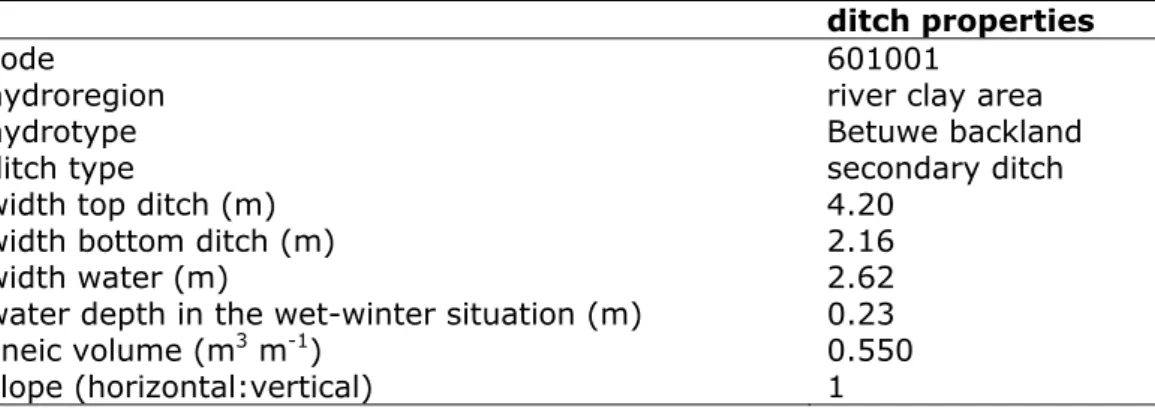
Calculations for this scenario have been performed using the proposed new exposure assessment methodology for the authorization of PPP in the Netherlands, as implemented in the DRAINBOW risk assessment tool (see Tiktak et al. 2012a, Tiktak et al. 2012b and van de Zande et al. 2012 for details). DRAINBOW includes emissions to surface water from drift as well as drainage. Details of the edge-of-field ditch derived for this scenario are given in Table 4-1. The ditch is characterized by the fact that the water flow
velocity is rather low most of the time.
The calculations are performed for a 15-year period (plus 5-year warm-up period4) and the year with the 63th percentile annual peak concentration in the
surface water is taken as the evaluation year. This scenario has not yet been approved for implementation and current PPP labels are possibly not fully compatible with this scenario.
Table 4-1 Characteristics of the ditch for the downward-directed spraying scenario (see Tiktak et al. 2012a).
ditch properties
code 601001
hydroregion river clay area
hydrotype Betuwe backland
ditch type secondary ditch
width top ditch (m) 4.20
width bottom ditch (m) 2.16
width water (m) 2.62
water depth in the wet-winter situation (m) 0.23
lineic volume (m3 m-1) 0.550
slope (horizontal:vertical) 1
Drift deposition on surface water in this scenario is calculated taking into account the appropriate drift curves for downward spraying (curves labelled ‘field crop’ and ‘field bare’ in Figure 7 of Tiktak et al. 2012a), assuming a total crop-free zone of 150 cm (i.e. including a 75 cm buffer) and 50% drift
reduction. Which curve is taken for the calculation of the drift deposition depends on the growth stage of the crop, as indicated by the BBCH code (Meier 2001). The approach is similar to a Step 3 approach as described in the FOCUS surface water guidance (FOCUS 2001), except that the Dutch
compulsory risk mitigation measures of using 50% drift-reducing technology (DRT) and a non-cropped buffer zone of 75 cm (total crop-free zone of 150 cm) are taken into account.
4 The procedure is analogous to the procedure used for leaching assessments (refs). The warm-up period and
Drainage is calculated using the preferential flow option of the PEARL model (Tiktak et al. 2012b). Water and dissolved substances may bypass the most active layer of the soil profile and reach the drainage system faster and in higher concentrations compared with results obtained without the
preferential flow.
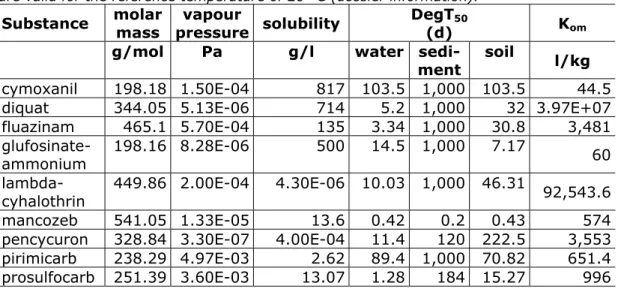
Calculations were performed for all substances listed in the tuber plant protection management scheme as proposed by PPO and given in Table 3-4 and Figure C - 13. Physico-chemical and fate properties of the substances used in the calculations are given in Table 4-2. These properties are taken from the Ctgbase (Dorgelo 2006). The Ctgbase contains endpoints of individual studies on the physico-chemical, fate and ecotox properties of PPP as supplied in the authorization dossiers. Table 4-2 gives appropriate central values (arithmetic or geometric means) of the approved data. If not available, the degradation half-life of a substance in sediment, DegT50sed, was set to a default value of 1,000 days, leading to negligible transformation in the sediment.
Table 4-2 Substance characteristics used in the tuber scenario calculations. All values are valid for the reference temperature of 20 °C (dossier information).
Substance molar mass pressure solubilityvapour DegT50
(d) Kom
g/mol Pa g/l water
sedi-ment soil l/kg
cymoxanil 198.18 1.50E-04 817 103.5 1,000 103.5 44.5
diquat 344.05 5.13E-06 714 5.2 1,000 32 3.97E+07
fluazinam 465.1 5.70E-04 135 3.34 1,000 30.8 3,481
glufosinate-ammonium 198.16 8.28E-06 500 14.5 1,000 7.17 60
lambda-cyhalothrin 449.86 2.00E-04 4.30E-06 10.03 1,000 46.31 92,543.6
mancozeb 541.05 1.33E-05 13.6 0.42 0.2 0.43 574
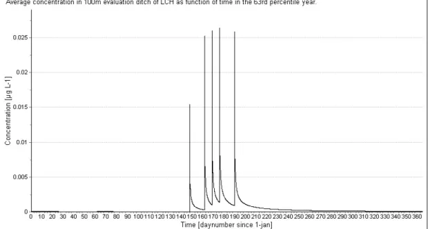
pencycuron 328.84 3.30E-07 4.00E-04 11.4 120 222.5 3,553 pirimicarb 238.29 4.97E-03 2.62 89.4 1,000 70.82 651.4 prosulfocarb 251.39 3.60E-03 13.07 1.28 184 15.27 996 Figure 4-1 gives an example of the predicted daily average concentration of lambda-cyhalothrin in the surface water of the edge-of-field ditch. Lambda-cyhalothrin is applied five times, with intervals of seven or 14 days. As can be observed, there is a slight accumulation of the substance in the water because the substance has not completely disappeared between the two applications. As expected, due to the high sorption coefficient of this
substance, the contribution of the drainage route to the concentration of the substance in the surface water is of minor importance.
Figure 4-1 Predicted daily average concentrations of lambda-cyhalothrin (LCH) in surface water in the edge-of-field ditch
4.1.2 Orchard scenario
As a new approach for upward and sideways spraying is still under
development, calculations for this scenario have been performed using the current methodology used for the authorization of PPP in the Netherlands, using the TOXSWA model, version 1.2 (Adriaanse 1996). In this methodology, emissions to surface water are caused by drift only, as other potential routes are not considered. Drift deposition values for a default crop-free zone of 3 m were used and the calculations were performed for a 1-year simulation period with no warm-up.
Details of the edge-of-field ditch derived for this scenario are given in Table 4-3. The ditch is characterized by the fact that the water flow velocity is constant, but differs between spring and autumn.
Table 4-3 Characteristics of the ditch for the orchard scenario (current NL standard ditch).
ditch properties
ditch type not defined
width top ditch (m) 4.00
width bottom ditch (m) 0.4
width water (m) 1
water depth in the wet-winter situation (m) 0.30
lineic volume (m3 m-1) 0.210
slope (horizontal:vertical) 1
Calculations were based on the standard drift percentages used in the authorization procedure in the Netherlands for fruit cultivation, without accounting for additional drift mitigation measures. For insecticide and fungicide sprayings, a distinction was made between trees without leaves (applications before May 1) and trees in full leaf (application after May 1).
For downward directed sprayings, the default value of 1% drift was used. The approach is similar to a Step 3 approach as described in the FOCUS surface water guidance (FOCUS 2001).
Calculations were performed for all substances listed in the orchard scenario given in Table 3-4 and Figure C - 11. The physico-chemical and fate
properties of the substances used in the calculations are given in Table 4-4, based on the Ctgbase (Dorgelo 2006). Table 4-4 gives the appropriate central values (arithmetic or geometric means) of the approved data. If not available, the DegT50sed was set to a default value, leading to negligible transformation in the sediment.
Table 4-4 Substance characteristics used in the orchard scenario calculations. All values are valid for the reference temperature of 20 °C (dossier information).
Substance molar
mass pressurevapour solubility DegT50 (d) Kom
g/mol Pa g/l water
sedi-ment l/kg amitrol 84.08 3.30E-05 340 93 10,000 54 bupirimate 316.42 1.60E-05 0.02 94 10,000 934 captan 300.59 4.20E-06 0.0049 0.16 10,000 48 difenoconazole 406.27 1.20E-07 0.0079 2.2 10,000 2,092 dithianon 296.32 1.41E-09 0.0002 0.28 1,000 1,478 dodine 287.45 1.00E-04 0.523 1.086 1,000 1,340 fenoxycarb 301.35 4.44E-07 0.0056 18.7 10,000 886 flonicamid 229.16 9.43E-07 5.2 33.8 10,000 0.94 glufosinate-amm. 198.16 8.28E-06 500 14.5 10,000 60 glyphosate 169.07 6.80E-06 0.0102 4.5 10,000 13,050 indoxacarb 527.84 9.90E-11 0.000166 25 10,000 894 kresoxim-methyl 313.36 2.30E-06 0.002 1.03 1,000 178.75 linuron 249.1 5.10E-03 0.0638 47 10,000 346 MCPA 200.62 1.20E-04 462 20.6 10,000 14.5 mepanipyrim 223.3 2.32E-05 0.0031 14.5 10,000 514 methoxyfenozi de 368.47 1.33E-05 0.0033 217 10,000 236 pirimicarb 238.29 4.97E-03 2.62 89.4 10,000 651.4 pyrimethanil 199.26 1.14E-03 0.0796 14.85 10,000 201 spirodiclofen 411.33 3.00E-07 5.00E-05 0.7 2.5 18,250 thiacloprid 252.72 3.00E-10 0.185 16.76 10,000 351.4 triadimenol 287.45 1.00E-04 0.523 1.086 10,000 1,340
Figure 4-2 gives an example of the captan concentrations in the surface water at the end of the ditch. The peak concentrations in the water reflect the application rates. Since captan has a low sorption coefficient, a decline of concentrations is due to transformation rather than to sorption to sediment. Due to the fast transformation of the substance in water, there is no build-up of the substance in the ditch.
Figure 4-2 Predicted daily concentrations of captan at the end of the edge-of-field ditch.
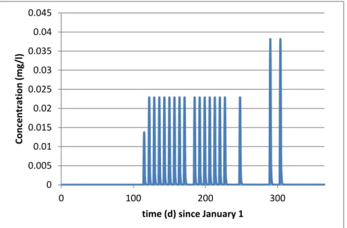
The modelled peak concentrations in surface water were used to calculate recovery times of Asellus aquaticus with the MASTEP model (See Section 4.2.3). Figure 4-3 shows concentration profiles and associated peak
concentrations of the selected substances used in the MASTEP calculations. 0 0.005 0.01 0.015 0.02 0.025 0.03 0.035 0.04 0.045 0 100 200 300 Concentration (mg/l)
Figure 4-3 Predicted exposure profiles of selected substances. The circles denote the peak concentrations that were evaluated regarding their effects on a population of Asellus aquaticus.
4.2 Impact assessment
For the evaluation of the potential risks of the concentration profiles of PPP used in the tuber and orchard scenarios, various types of ecotoxicological data have been collected from both dossiers and other sources. The data were used in three effect assessment models to assess ecotoxicity of separate substances and their mixtures, representing three tiers of
increasing modelling refinement. The three used models were an approach
Tuber exposure profiles
Orchard exposure profiles
0.001 0.01 0.1 1 Concen tr ation ( μ g/ L) Date Dithianon 0.1 1 10 100 Concen tr ation ( μ g/ L) Date Dodine 0.01 0.1 1 10 Concen tr ation ( μ g/ L) Date Thiacloprid 0.01 0.1 1 10 Co n ce n tr at io n ( μ g/ L) Date Fluazinam 0.01 0.1 Con ce n tr at ion ( μ g/ L) Date Lambda-cyhalothrin
species sensitivity distribution modelling, SSDs), and a population-modelling approach (evaluating potential impacts on a selected species, the model is named MASTEP).
The source of the dossier data was, for most of the substances, the data provided to the Board for the authorization of pesticides and biocides (Ctgb) or the European Food Safety Authority (EFSA). In a few cases, supplemental data were obtained from databases like Agritox (database of l’Agence
nationale de sécurité sanitaire de l’alimentation, de l’environnement et du travail (Anses)) and Footprint (www.eu-footprint.org), or by personal communication with Ctgb.
For constructing species sensitivity distributions (SSDs) and the calculation of the multi substances Potentially Affected Fraction (msPAF), information from several literature sources was used, but often data collected within the framework of setting (Dutch) environmental quality standards (EQS) could be used (these data are not provided in this document).
4.2.1 Toxic Unit (TU) approach
In order to estimate the joint risks of the PPP in the two different application scenarios, the results from the fate modelling were first evaluated via Toxic Unit (TU) calculations.
Evaluating (aggregated) Toxic Unit is simple and straightforward. It consists of determining the ratio of a measured or predicted environmental
concentration (here: the PEC) and an ecotoxicity endpoint (e.g., NOEC, or EC50 or else), so that values >1 signal insufficient protection against the selected ecotoxicity endpoint. When using the concept in cumulative
assessment, the evaluation consists of linear summation of Toxic Unit values over the different substances. This is an approach that utilizes Concentration Addition (CA) modelling to address the expected mixture exposure, with the implicit assumption of a linear dose-response curve for all substances, and with higher sum-TU values suggesting higher risk, and again a critical sum-TU value of 1. The review of Kortenkamp et al. (2009) refers to the CA model as a default mixture model approach, though it is one that may have a tendency to overestimate risks, unless a mixture induces specific synergistic effects. The CA-concept is further based on the assumption that all substances have the same mode of action and that different substances do not interact on a physico-chemical level or in their kinetics or toxicodynamics (Backhaus and Faust 2012).
TU calculations were done by dividing the PEC for each substance in a mixture on each day by the lowest L(E)C50 separately for each of the three trophic levels in the base set, i.e. primary producer, crustacean and fish resulting in a TUprimary producer, a TUcrustacean and a TUfish. When more than one value for the same species was available, the geomean value of these values was calculated before selecting the lowest value. Subsequently, the values for the individual substances were summed to one ΣTU-value for each trophic level for each day.
4.2.2 Mixture toxic pressure (msPAF) approach
A more sophisticated approach to quantify the predicted joint toxicity of a mixture is called the mixture toxic pressure method, as proposed by (De Zwart and Posthuma 2005). This method makes use of the available toxicity
data for a substance for all species of which ecotoxicity data are known, instead of taking the lowest or geomean of the base set species. Available data are assumed to be a representative sample from the distribution of sensitivities towards a substance in an ecosystem. The data can then be used to calculate the proportion of species at risk at a certain predicted toxicant concentration, PEC, yielding the so-called toxic pressure for every substance for which there is a PEC, and expressed as Potentially Affected Fraction of species (PAF). This outcome bears a relationship with biodiversity effects, according to various validation studies, especially when the SSD is constructed from effect data such as LC50s or EC50s. In this study LC50s and EC50s were used to construct SSDs, and likewise, the toxic pressure that is derived is expressed as PAFEC50.
First, a SSD EC50 is created per substance using the ETX 2.0 software (van Vlaardingen et al. 2004). This program calculates the average and standard deviations of the log10-transformed ecotoxicity values, as well as the hazardous concentration for 5% of the species (HC5, EC50), assuming a log-normal distribution of the ecotoxicity data. In cases in which only one or two toxicity data were available, the HC5 was estimated using the geometric mean of the HC50/HC5 ratio of all other substances as an extrapolation factor. When only one data point was available, this value was used as the best estimate of the HC50. In cases of two values, the geometric mean was used. For the tuber scenario, the extrapolation factor to estimate the HC5 on the basis of the HC50 was 15. For the orchard scenario, it was a factor of two higher because of the limited number of available data for the selected substances (Table 4-5).
The SSD for a substance and a selected test endpoint (e.g., the EC50) is determined by two parameters, Xm and Sm:
Xm the concentration at which the effect criterion (e.g. L(E)C50) is
exceeded for 50% of all species tested. In practice, this is the median of the toxicity data of the data set.
Sm the slope of the curve. In practice, this is the standard deviation of log(Xm). An extrapolation factor was used when only one or two data were available.
The toxic pressure for a certain concentration of a substance (PEC) can be calculated using the Excel NORMDIST function, and expressed as PAF: PAF = NORMDIST(log(PEC), log(Xm), Sm, 1)
If the toxicity values for a certain substance show that a particular
taxonomic group of species is more sensitive (factor >10 according to (Brock et al. 2011) than the rest, then the toxic pressure has been calculated for that particular sensitive group, i.e., by utilizing the same modelling steps, but then for ecotoxicity data for the selected taxonomic group only. This yields the estimated toxic pressure for a taxonomic group, PAFtaxonomic group. The PAF values for single substances are combined into the mixture toxic pressure of a situation (expressed as msPAF) for all substances (a,b,…,n) by using the formula (De Zwart and Posthuma 2005):
The approach of De Zwart and Posthuma describes an option for aggregating toxic pressures over substances within both ‘subgroups of substances with similar modes of action’, and ‘across such groups’. The above formula represents the approach for substances with different modes of action. This formula was applied in the current study.
Table 4-5 Arthropod SSDLC50 parameters of the substances as used in the calculations
including estimated 5th percentiles and ratios of peak PECs and the estimated 5th
percentiles (n=number of test data underlying the mean and standard deviation).
mean μ (log10 LC50) standard dev. ∆ (log10 LC50) n HC5, LC50 (μg/L) max peak /HC5(-) tuber scenario λ-cyhalothrina -1.12 0.71 21 0.0050 6.73 pencycuron 2.48 NA 1 20c 0.25 fluazinama 1.92 0.62 7 7.02 0.17 mancozeb 3.25 0.63 3 105 0.08 prosulfocarb 3.00 0.10 5 659 0.02 diquat 3.69 1.13 13 62.1 0.01 glufosinate 4.60 0.93 9 1,039 0.00 pirimicarb 4.23 1.20 15 1600 0.00 cymoxanil 4.58 NA 1 37,831 0.00 orchard scenario dithianonb 1.12 NA 1 0.439c 8.07 spirodiclofen > 1.57 NA 1 > 1.23c < 3.59 dodineb 2.35 NA 2 7.46c 3.23 thiaclopridb 1.38 0.906 12 0.701 2.77 kresoxim 2.08 NA 2 4.01c 0.83 methoxyfenozide 2.4 0.882 6 7.25 0.44 fenoxycarb 2.29 1.2 4 1.23 0.38 indoxacarb 2.26 NA 2 6.07c 0.16 bupirimate 3.28 NA 1 63.5c 0.11 captan 3.52 0.452 7 541 0.07 pirimicarb 4.23 1.2 15 160 0.05 pyrimethanil 3.53 NA 2 113c 0.03 triadimenol 3.4 NA 1 83.7c 0.02 difenoconazole 2.89 NA 1 25.9c 0.02 linuron 3.19 0.887 7 45.5 0.01 amitrol 4.55 1.01 7 642 0.01 glyphosate 4.48 0.779 8 1375 0.01 glufosinate 4.85 NA 2 2360c 0.00 MCPA 5.33 0.212 3 83870 0.00 flonicamid > 5 NA NA > 3333c 0.00
a selected for tuber scenario effect simulations (see Section 4.2.3) b selected for orchard scenario effect simulations (see Section 4.2.3) c extrapolated value, see text for further explanation
4.2.3 The MASTEP population model
We used the MASTEP population model for a selected species, Asellus aquaticus for simulating the population dynamics of impacts and recovery over time, given the time-dependent PEC patterns (Galic et al. 2012). In the model, Asellids are individually simulated using stochastical input
parameters for key ecological parameters of the species, amongst which proliferation time and natural mortality (van den Brink et al. 2007). All population parameter values were used as given in the model description (Galic et al. 2012). Individual movement was taken as the only locomotion process.
The modelled environment consisted of a 1,000 m long and 1 m wide watercourse, where exposure over time was assumed to happen only in the first 300 m. The boundary conditions were periodic, so that the end of the watercourse was directly connected to the beginning, thus mimicking
upstream and downstream sections. PPP concentrations were taken from the DRAINBOW and TOXSWA model results for the tuber and fruit scenario, respectively.
Dose response function
Pesticide-induced mortality was calculated by using the logistic
dose-response relationship, which is standard in ecotoxicological studies (Rubach et al. 2011):
= 1
1 + ∙( )
whereby C (μg/L) is a given exposure concentration (predicted as PEC), LC50 (μg/L) is the lethal concentration leading to 50% mortality, slope (-) is the steepness of the dose response relationship, and m is mortality (%). Mortality rates were calculated for each day in response to the given changes in the predicted exposure concentrations, and a corresponding number of randomly chosen individuals were removed from the population. Monte Carlo sampling and simulations
For assessing the variability of sensitivities of aquatic macro-invertebrates towards the different pesticides, we simulated the population dynamics and pesticide effects in a Monte Carlo style. We varied the sensitivities of the simulated populations by generating random LC50 values. The LC50 values were constructed by drawing random numbers ri from a normal distribution with parameters mean value μ and standard deviation σ and then raising r to the power 10:
, = 10
As parameters of the normal distribution used for the Monte Carlo sampling of the LC50 values, the effect simulations, mean value and standard
deviations of the log10-transformed LC50 data were used (Table 4-6). For each of the drawn LC50 values, pesticide effects and populations dynamics were simulated in 10 replicates.
simulated exposure dynamics, the slopes were taken from the literature, when available.
The slope of the dose-response function was calculated, when available, from literature data by the formula:
=
1− 1 ( ) −
whereby p (-) is a given percentage of mortality and Cp is the associated concentration. Using p values different from 0.5, e.g. LC10 or LC90 values, the slope can be calculated from respective data. For lambda-cyhalothrin and fluazinam, respective data was available (Schroer et al. 2004, van Wijngaarden et al. 2010) and the slopes have been calculated (Table 4-6). For dithianon, dodine and thiacloprid, no such data was available, so we used a slope with a default value of 2. We checked the sensitivity of the mortalities for the peak concentrations of the three substances and found a variation of the mortalities of 10% at maximum (results not shown).
Choice of substances for effect simulations
The ratio PECmax/HC5, LC50 was used for ranking of the substances
concerning the expected effects. For the tuber scenario, it was decided that substances with only one toxicity value (pencycuron) would be excluded, while all other substances with a PeakConc/HC5, LC50 ratio larger than 0.1 were included (lambda-cyhalothrin and fluazinam, Table 4-5). For the
orchard scenario, all substances with a PeakConc/HC5, LC50 ratio larger than 1 were included, except spirodiclofen for which only a “greater than” toxicity value was available. The cut-off criterion for the orchard was set higher in order to limit the number of simulations. Table 4-6 lists all the parameters used to describe the distributions of the toxicity (LC50) values and the slope used to describe the full dose-response relationship. The toxicity was
included in a probabilistic way in terms of LC50, the slope was deterministic.
Table 4-6 Parameters of the pesticides as used in the MASTEP simulations.
mean μ (log10 LC50) standard dev. σ (log10 LC50) slope day of 1st exposure max peak (μg/L) tuber scenario λ-cyhalothrina -1.12 0.71 2.43a 148 0.03 fluazinamb 1.92 0.62 1.82b 169 1.23 orchard scenario dithianon 1.12 0.62c 2d 92 3.55 dodine 2.35 1.24 2d 88 24.1 thiacloprid 1.38 0.906 2d 141 1.93
a calculated from Schroer et al. 2004
b calculated from van Wijngaarden et al. 2010 c average of the standard deviations of all substances d default value
Simulation scenarios
For the tuber scenario, we performed simulations with lambda-cyhalothrin and fluazinam alone and the mixture of the two, while for the orchard scenario the effects of dithianon, dodine and thiacloprid were simulated individually, as well as for the mixture of the three substances.
The mixture toxic effects were simply estimated by adding the single
substance mortalities. In practical terms, that only resulted in more frequent exposures, because the time points of exposure peaks were different for the single substances.
For each pesticide, a control scenario without exposure was simulated in 100 replicates and, for each of the Monte Carlo (MC) permutations, population effect dynamics were simulated in 10 replicates. For evaluation, the average of the 100 control simulations and the average over 10 replicates of each MC permutation were used.
The time course of the average of each 10 replicates for one LC50 value was divided by the mean of the controls, which yielded the relative abundances. This relative abundance is 1 for no effect of the substance and smaller than 1 for a negative impact. Monte Carlo simulations were performed with 1,000 permutations for the tuber and with 1,400 permutations for the orchard scenario. From these 1,000 or 1,400 simulated time series, the average and some percentiles were calculated and visualized.
Recovery times
From the simulated time series, population recovery times were calculated as follows. For a defined threshold T=0.9 and a defined effect starting day (Table 4-6), we observed how long (d) it took for the relative abundance to be larger than the threshold again. To deal with the stochastic fluctuations of the simulated values, we considered recovery to be reached when on five of 10 consecutive days the threshold was exceeded. The distribution of these recovery times was plotted in so-called violin plots or kernel-density plots to illustrate the distribution of the data.
4.3 Results
4.3.1 Toxic Unit (TU) approach 4.3.1.1 Tuber scenario
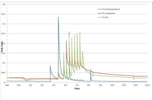
Figure 4-4 displays the results of the TU calculations for primary producers, crustaceans and fish in the tuber scenario. A per substance TU > 1 means that the acute 50%-effect threshold is exceeded. Taking into account a TER of 100 for crustaceans and fish according to the aquatic risk assessment under 1107/2009/EC, a TU value of 0.01 could be distinguished as a trigger value above which adverse effects may occur on the group of crustaceans and fish. Based on the TER of 10 for primary producers, a trigger value of 0.1 TU could be used for primary producers. The calculations show that, depending on the substance, different trophic levels are affected, while the ΣTU value never exceeds the value of 1. Figure 4-5 to Figure 4-7 show the results for the separate trophic levels and individual PPP.
Figure 4-4 Aggregated Toxic Unit values (LC50-based) for the three trophic levels during time in the tuber scenario.
Primary producers are mainly at risk due to exposure to pencycuron (- line) and prosulfocarb (- line) in spring and to mancozeb (- line) later in the season (Figure 4-5). For primary producers, the trigger value of 0.1 is exceeded only shortly after the applications of prosulfocarb and mancozeb. The level of risk decreases very rapidly after application of these substances.
Figure 4-5 Toxic Unit values (LC50-based) for individual substances and the aggregated exposure scenario for primary producers during time in the tuber scenario.
Crustaceans are most at risk due to exposure to pirimicarb and lambda-cyhalothrin and, to a lesser extent, to mancozeb (- line) (Figure 4-6). For crustaceans, a TU value of 0.01 could be distinguished as a trigger value above which adverse effects may occur on the group of crustaceans. This value of 0.01 is exceeded from the first application in the year up to the end of the year.
Figure 4-6 Toxic Unit values (LC50-based) for individual substances and the aggregated exposure scenario for arthropods during time in the tuber scenario.
Fish are mainly at risk due to exposure to lambda-cyhalothrin (- line) and, to a lesser extent, to mancozeb (- line) and fluazinam (- line) (Figure 4-7). The threshold value of 0.01, which according to EFSA (2013) also pertains to fish, is exceeded from May, after the first PPP application, to the end of the year.
4.3.1.2 Orchard scenario
Figure 4-8 shows the results of the ΣTU calculations for the orchard
scenario. It shows that the different trophic levels (i.e. primary producers, crustaceans, fish) are indicated to be at risk because of different substances in the mixture.
Figure 4-8 Aggregated Toxic Unit values (LC50-based) for the three trophic levels during time in the orchard scenario.
Figure 4-9 to Figure 4-11 show the TU values split up for the different trophic levels and the different pesticides. The graphs show that the relative influence of the different substances may vary during the year. The group of primary producers (Figure 4-9) is at risk mainly in the spring (> 98%) due to exposure to dodine (- line), later in the season due to exposure to linuron (- line, >93%) and, to a lesser extent, to spirodiclofen (- line, maximum 47%) and captan (- line, maximum 21%). Dodine, linuron, spirodiclofen and captan are the main contributors to the toxicity.
For primary producers, a TER of 10 is taken into account in the acute risk assessment under Regulation 1107/2009/EC (EFSA 2013). This means that a TU of 0.1 could be regarded as a threshold, above which significant adverse effects may occur with respect to this group of organisms. This threshold value is exceeded during a relatively long period running from day 150 to 190, merely caused by linuron, and during a few shorter peaks, caused by dodine and captan. Most peaks in the TU values are caused by one dominant substance. The contribution of other substances is minimal. Only linuron and its adherent effects on the group of primary producers is present for a relatively long time in the water column.
Figure 4-9 Toxic Unit values (LC50-based) for individual substances and the aggregated exposure scenario for primary producers during time in the orchard scenario.
Figure 4-10 shows the TU-values for crustaceans resulting from PPP-application in the orchard scenario. Crustaceans are mainly affected by dithianon (- line, 67%) and dodine (- line, 33%) in the spring and pirimicarb (- line, maximum 30%) and thiacloprid (- line, >97%) later in the season. Taking a TER of 100 into account for crustaceans according to the aquatic risk assessment under Regulation 1107/2009/EC, a TU value of 0.01 could be distinguished as a trigger value, above which adverse effects may occur on the group of crustaceans. This value is exceeded in spring for three short periods of a few days and for a long period running from day 125 to 300, mainly caused by the cumulative effect of thiacloprid and pirimicarb. For this trophic level, a combined effect of the different substances is more
pronounced than it is for the group of primary producers. This could be caused by the fact that, during the year, more insecticides than herbicides are applied.
Figure 4-11 shows the TU-values for fish due to PPP-applications in the orchard scenario. Fish are mainly affected by spirodiclofen in the spring (- line) and, due to a combined effect of fenoxycarb (- line) and captan (- line), later in the season. The threshold value of 0.01, which according to EFSA (2013) also pertains to fish, is exceeded for a long period in the year, starting from day 115 (application of spirodiclofen) and running up to day 330 after the last application of captan. Also for this trophic level, a more
pronounced combined toxicity is predicted.
Figure 4-11 Toxic Unit values (LC50-based) for individual substances and the aggregated exposure scenario for fish during time in the orchard scenario.
4.3.2 Mixture toxic pressure (msPAF) approach
Figure 4-12 displays the acute (mixture) toxic pressure results for the tuber scenario. As can be seen, for most of the time >90% of the total toxic pressure (msPAFLC50) is caused by the single substance pressure by lambda-cyhalothrin (- line). Only during a short time, cymoxanil (- line) also
contributes to the acute mixture toxic pressure for a maximum of 30% in the beginning of June. However, in that period, the acute mixture toxic pressure value is relatively low. Later in the season, the acute mixture toxic pressure value is substantially influenced by diquat-dibromide (- line), related to an exposure that exceeds the HC5, LC50 for a short time. The acute mixture toxic pressure value of 0.05 is exceeded only for a few separate periods.
Figure 4-12 Temporal variation of the toxic pressure of individual substances and the total mixture (expressed as acute msPAF) over a full year for the tuber scenario. The red line is a selected criterion, marking when it is predicted that more than 5% of the species would be affected beyond their LC50; the Y-axis can be interpreted as a relative predictor of species loss due to (mixture) exposure.
Figure 4-13 displays the acute mixture toxic pressure results for the orchard scenario. A closer look at the results shows that dodine (- line) has a
relatively high contribution to the total toxic pressure in the spring, followed by a high peak caused by spirodiclofen (- line) and a longer period of relative high mixture toxic pressures caused by a combination of captan (- line) and thiacloprid (- line). As a result, the predicted acute mixture toxic pressure exceeds the selected value of 0.05 during a large part of the growing season. This value of 0.05 may be seen as a trigger value, above which adverse effects on the ecosystem may occur. The Y- axis – given the use of LC50-values to derive the mixture toxic pressure – can be seen as a
predictor of species loss due to (mixture) exposure.
Figure 4-13 Time-dependent change of the acute mixture toxic pressure values over a full year for the orchard scenario.
Figure 4-14 shows the predicted change in abundance of a species over time for the individual substances and their mixtures. For the tuber scenario, lambda-cyhalothrin resulted in long-term effects on the population size of the modelled species, while fluazinam hardly resulted in any effects.
Figure 4-14 Effects relative to control for individual substances and combinations expressed as relative abundance changes (1=initial population size). Scenarios: tuber (a: fluazinam, b: λ-cyhalothrin, c: combination); orchard (d: dithianon, e: dodine, f: thiacloprid, g: combination). Dashed vertical lines indicate exposure events. Grey shaded areas: between the 10th and 90th percentiles. Thick solid lines:
The effect sizes of the mixture of both substances in the tuber scenario are almost identical to the ones for lambda-cyhalothrin only. This absence of interaction on effect size and recovery of the mixture of substances used in the tuber scenario is also shown by the distribution of the recovery times (Figure 4-15). Both the fractions of simulations where the population was affected (0.63 and 0.64 for lambda-cyhalothrin and the mixture, respectively) and the median recovery times (349 and 344 days for lambda-cyhalothrin and the mixture, respectively) were not really different between the runs with lambda-cyhalothrin only and the mixture.
In the orchard scenario, the applications of the three substances alone resulted in large effect sizes just after exposure (Figure 4-14). The mixture shows increased effect sizes after the exposure events to the three substances between days 78 and 141. The recovery times, however, are not higher for the mixture compared with those associated with exposure to the individual substances (Figure 4-15). The chance of having an effect is, however, much higher when the population is exposed to the mixture (80%), compared with the individual substances (27 – 45%). The shorter median recovery time for the mixture can be ascribed to the higher fraction exposed slightly above the levels that result in effects.
Figure 4-15 Recovery times (Y-axis, in days) for individual substances and their mixtures for the tuber and orchard scenarios. The numbers in the figure give the median recovery times. The number below the density plots denotes the percentage
5
Discussion
In this report three methods, of increasing complexity and probable
specificity and precision, are used for assessing the impact of simultaneous, consecutive and/or repeated applications of PPP in the growing season of crops. For all three methods, the results can be assessed regarding the
question whether cumulative exposures expectedly result in higher impacts. We applied the Toxic Unit approach by using the basic acute toxicity dossier data for primary producers, invertebrates and fish in combination with the default toxicity exposure ratios of 0.1 for primary producers and 0.01 for invertebrates and fish. The mixture toxic pressure approach was applied based on acute-LC50 species sensitivity distributions, separate for specific groups of organisms, and the fraction of species potentially affected by the mixture was determined. Due to the use of the LC50-ecotoxicity endpoint in this model, the predicted (mixture) toxic pressures likely closely relate to the fraction of species lost due to predicted (mixture) exposures. The MASTEP-model was applied to include recovery in the assessment, by also
considering the potential for population recovery upon peak exposures to individual PPP, applied in a realistic sequence.
Both the TU and the msPAF approach provide more information how
simultaneous and/or consecutive applications result in combined toxic stress. These approaches allow the use to identify if the combined use will exceed trigger values (where single use does not) and in case of the msPAF, what fraction of species would be affected.
It is noted that, even for some single substances, a potential risk is identified, despite the fact that these substances are authorized for the uses considered in this report. There are several reasons that may cause this discrepancy. The effect data used in this study are solely based on acute laboratory toxicity studies on base set species, while in the authorization process higher tier methods, such as mesocosms or other semi-field studies, may have been used as well. For the tuber scenario, state-of-the art exposure modelling was applied. The newly developed DRAINBOW model differs from the models currently used in the authorization process, but is considered more appropriate because it includes drainage and realistic adaptations such as lower water velocities during part of the year, which leads to slower
dissipation. Furthermore, drift values were obtained from newly derived drift deposition curves (van de Zande et al. 2012) and additional,
substance-specific drift mitigation measures were not taken into account. Such additional substance-specific drift mitigation measures may have been applied in the authorization process and laid down in the use instructions.
Both the TU approach and the mixture toxic pressure approach indicate that mixtures may have higher effects than single substances. In most cases, however, one or a few substances dominate the combined effect. This phenomenon is also frequently observed in other contexts (e.g., the ongoing EU-project SOLUTIONS, preliminary data analyses. See also Van Broekhuizen et al. 2017).