An analysis of the applicability of games in an Operations Management course

(1)

AN ANALYSIS OF THE APPLICABILITY

OF GAMES IN AN

OPERATIONS MANAGEMENT COURSE

Word count: 26.537

Klara Sabbe

Student number: 01503257

Supervisor: Prof. Dr. Veronique Limère

Master’s Dissertation submitted to obtain the degree of:

Master in Business Engineering: Operations Management

Academic year: 2019-2020

(2)

CONFIDENTIALITY AGREEMENT

PERMISSION

I declare that the content of this Master’s Dissertation may be consulted and/or reproduced, provided that the source is referenced.

(3)

PREAMBLE

The COVID-19 crisis had no extreme influence on this research. The initial research study with games had not yet been worked out, so an adjustment to an online research was quickly made. Due to the fact that every research had to be conducted online from now on, respondents were inundated with questionnaires. Because of this, the enthusiasm of students was perhaps a bit lower to fill in again another questionnaire. In addition, the libraries were closed, so some sources were not available. However, after a while electronic scans could be requested.

A quick ventilation and distraction with fellow students was not possible, but the good care of my parents made up a lot. The COVID-19 crisis however, ensured that the full attention could go to the master dissertation

(4)

FOREWORD

This dissertation is the final step to obtain my Master Degree Business Engineering at the University of Ghent. Throughout my studies I have learned a lot and I am very grateful for the many people I have met. Of course there were some difficult and stressful moments, but most of all I experienced many unforgettable moments. It were 5 valuable years during which I not only developed myself intellectually, but also personally.

Writing this dissertation would not have been possible without the help of a few people. First of all, I would like to thank my supervisor Prof. dr. Veronique Limère to be available whenever I had questions and to guide me through this process. I would also like to thank my family and friends for their support, not only during this whole masters dissertation process, but also for the past years. The last few months have been an unusual and special period, but luckily we could stay connected and found support and courage online.

Klara Sabbe June 2, 2020

(5)

LIST OF ABBREVIATIONS

OM Operations Management

PPC Production planning and control WS Workstation

SC Supply chain WIP Work in progress

(8)

LIST OF FIGURES

Figure 1: Gamification framework (Deterding et al., 2011) ... 4

Figure 2: Four stages of the learning cycle (Kolb, 1984) ... 8

Figure 3: Board layout Beer Game (Universität Klagenfurt) ... 12

Figure 4: Worksheet assembly process (Klotz, 2011) ... 22

Figure 5: Assembly process Littlefield Technologies (Responsive Learning Technologies 2014) ... 30

Figure 6: Game layout Medica Scientific Processim Lab ... 44

Figure 7: Initial parameters SodaPop Game ... 56

Figure 8: Demand pattern SodaPop Game... 57

LIST OF TABLES

Table 1: Starting inventories MRP ... 18

Table 2: Starting inventories JIT ... 19

Table 3: Starting inventories CONWIP ... 19

Table 4: Starting inventories TOC ... 19

Table 5: Examples of lean games ... 24

Table 6: Overview games ... 53

Table 7: Respondents according study field that completed the full test ... 58

Table 8: Respondents according study field that only filled in the pre-test ... 59

Table 9: Average scores of pre-test ... 60

Table 10: Comparison pre- and post-test results (mean values) ... 62

(9)

LIST OF GRAPHS

Graph 1: Average grouped results ... 60 Graph 2: Student responses ‘evaluation of game’ ... 63 Graph 3: Student responses learning efficiency ... 64

(10)

I. INTRODUCTION

Gaming has been around for a very long time. Children learn a lot by playing games. Older people play in their spare time and for pleasure. When hearing the term ‘game', many people think of Monopoly or Scrabble, but games are also more widely used – for example in business life, where they are used to encourage employees to get more physical movement during working hours by using apps, a credit system or leader boards. Companies are also using games in their application procedures to test how risk averse a candidate is. Business games that imitate an economic situation are also used in trainings and help learning employees to make strategic decisions. So, why not also use games in (higher) education?

For groups with a large number of students, traditional lectures are the most common way of teaching. Conventional classes often focus on giving definitions, passively applying information on certain topics and using formulas in exercises or individual tasks (Chwif & Pereira-Barretto, 2003). In this way students learn in a passive way, which prevents them from actively participating in the learning process. By shifting the focus to a more student-centered approach of learning which focuses on experiences – like the use of games and simulations - students become more actively involved in the course content and will be more motivated (Fish, 2007).

Also in the area of Operations Management (OM) it is not always easy to motivate students and to allow them to actively participate in the lessons, as they have little experience and could have difficulties in placing the concepts in a broader context (Satzler & Sheu, 2002). Through the use of integrated games, students get a first, simplified and risk-free experience on how the real business world works. They can “apply theoretical knowledge to complex practical situations in a controlled environment” (Gundala & Singh, 2016, p. 2). Scenarios can be set up to simulate specific situations, one can experiment with decision-making, and several solutions can be tested and compared to each other

This research focuses on existing games that can be applied in an introductory course of Operations Management, given to a large group of undergraduate students. The target groups considered are 3rd_{bachelor students Business Engineering, Business Economics and Business Administration at} the University of Ghent. An average of 230 students from the first group mentioned, and 550 students from the last two, participate in the course annually.

This research investigates which games could be feasible towards this large group of students. Consideration is given to limited space and movement possibilities, to the time frame which is limited in-class to 3 hours, and to the logistical and organisational aspects of using games during the lecture.

(11)

A concrete study will be set up to determine to what extent students are open to playing games in the Operations Management course. A specific game is chosen and played by students in order to obtain information about the students' perception about the use of games as a (partly) replacement of a classic lecture and to check whether this initial feeling changes after being presented to a short game. In this way it can be analysed whether the use of a game would be useful in the Operations Management course to stimulate students’ motivation.

This master dissertation contains five parts. In this first part the aim of the research is explained. In part two, a brief explanation is given of what is meant by the use of games in education, followed by a section on motivation and a concise comparison between manual games and digital games. Part three covers specific games that might be eligible to be applied in the Operations Management course. A distinction is made between manual games and digital simulations. The games are briefly compared with each other and suggestions are given for the best applicable ones. Part four includes the research study in which the SodaPop Game of GameLab Education is used to determine the initial perception of students in regard to the use of games in the OM course. The effect of the game and the game itself will be analysed. The master dissertation ends with a discussion of the limitations and further research.

(12)

II. LITERATURE REVIEW

What are games?

1.1 Gamification framework

Gamification is defined as “the use of game elements in non-gaming contexts to improve the user experience and engagement” (Deterding, Dixon, Khaled, & Nacke, 2011). A serious game according to Michael and Chen (2006) is “a game in which education (in its various forms) is the primary goal, rather than entertainment”. These two concepts share a number of aspects, yet are not completely the same.

There is a difference between gamification, serious games, toys and a playful design. According to Caillois (2001), the first distinction can be made between play and game, referred to as ‘paidia’ and ‘ludus’. ‘Ludus’ or ‘gaming’ includes playing in a competitive manner with guidelines, rules and tactics towards an objective, for example winning or losing the game. Whereas ‘paidia’ or ‘playing’ implies a wider and more loose concept including the interactions and environment for playfulness. The word ‘element’ in the definition of Deterding (2011) is important for the second difference between the concepts, namely the use of ‘whole’ games or specific ‘elements’ or ‘parts’ of the game. A software program used in daily situations may incorporate some game ‘elements’ (e.g. badges, points, leader boards) in order to make the use of it more enjoyable (Matallaoui, Hanner, & Zarnekow, 2017), whereas the ‘whole’ refers to full-fledged and complete games. Deterding et al. (2011) make use of four quadrants to illustrate this difference between game and play (defined on the y-axis) and between ‘whole’ versus specific ‘parts’ of games (indicated on the x-axis). Those four components make up a model with four different kind of games (Figure 1).

Toys are set up from the beginning till the end and are complete, used in playful contexts without the typical rules and boundaries of a game. Similar to toys, the playful design is used in playful situations leaving room for improvisation, but incorporates only some game elements. Serious games are – as implied within the term – used in more serious contexts with a goal that goes beyond amusement. These are complete games and are often used as simulation, e.g. in military or educational training. They are set up according to the game structure and incorporate learning value in addition to entertainment. Gamification is again part of the ludus and makes use of gaming elements in a competitive and structured environment (Deterding et al., 2011). Different game techniques such as points, badges, bonusses or other rewards are used to increase motivation and to create a competitive environment.

(13)

Figure 1: Gamification framework (Deterding et al., 2011)

There is quite some confusion about the word ‘gamification’ which often results in an incorrect use of the term. Gamification and serious games both try to achieve a goal that is more than just playfulness and their difference is subtle. Serious games have a holistic approach that responds to the overall behaviour and commitment of players. Specific rules need to be followed and particular actions are needed to get to the end result (Oliveira & Petersen, 2014). Gamification, on the other hand, can exist without a real game. Gamification elements are used in daily situations to guide and motivate players to adopt a certain behaviour (Oliveira & Petersen, 2014).

‘Toys’ and ‘playful-design’ are beyond the scope of this research, which focuses on the implementation of full games into lectures. As a result, ‘gamification’ will not be reviewed either. Some elements of it, however, might occur in the discussion below.

1.2 History serious games

Abt (1970) was the first who gave a formal definition of serious games which is closely related to the meaning nowadays, and defines it as follows: “These games have an explicit and carefully thought-out educational purpose and are not intended to be played primarily for amusement” (Abt, 1970, p. 9). In his book ‘Serious Games’ he describes the concept of serious games with the main goal to use it during trainings and in education (Abt, 1970). Abt explains several non-digital ‘pen and paper’ games, but he made also the transition to digital games. For example, the TEMPER game was developed by Abt and the Raytheon Company as a computer simulation of a cold war conflict. This simulation model was unique as it covered a worldwide scope and complex interactions between different nations and regions (Forces, 1968). Sawyer (2002) increased the popularity of the term. In collaboration with David Rejeski he wrote the white paper “Serious games: Improving public policy through game-based learning and simulation”. It enhances the improvement of simulation games for policy making by use of the technology and knowledge obtained from video

(14)

games (Sawyer & Rejeski, 2002). Rapidly followed, together with The Woodrow Wilson Centre he co-founded the ‘Serious Games Initiatives’ which promotes the development of games in the field of policy and management topics. It is still one of the leading organisations in the serious games market (Wilsoncenter, n.d.). Also, in 2002 the U.S. Army launched the free digital game ‘America’s Army’. The game was designed as a recruitment tool in which training sessions are simulated and where players can act as militaries. In this way, young people are informed about what the military looks like (Gudmundsen, 2006). This game together with the Serious Games Initiatives created great public interest in serious games. The year 2002 is therefore known as the starting point of the 'new wave' of serious games (Djaouti, Alvarez, Jessel, & Rampnoux, 2011). The military sector has a long background with regard to serious games, but the development of games also occurred in other important sectors such as politics, corporation, education and the healthcare industry, to name a few (Michael & Chen, 2006).

(15)

Motivational aspect

2.1 Self-Determination Theory

Developing serious games can be challenging as the games have to motivate players as well as serve as an educational tool. Engaging and motivating students is one of the most important drivers to teach students successfully (Buckley & Doyle, 2014). The Self-Determination theory of Deci and Ryan (Deci & Ryan, 1985; Ryan & Deci, 2000) recognises different types of motivation based on the aim and goal of an action. The most important distinction is made between intrinsic and extrinsic motivation. Intrinsic motivation refers to taking actions related to inherent interest and leading to inherent satisfaction and pleasure (Ryan & Deci, 2000). Students who are intrinsically motivated are interested in what they learn as well as in the process it entails (Harlen & Deakin Crick, 2003). The intrinsic motivation emerges from an interest in the subject and reflects a personal goal. Extrinsic motivation refers to behaviour based on achieving external goals or benefits or avoiding punishments. It is driven by external rewards or pressure (Ryan & Deci, 2000). Extrinsic engaged students are engaged in learning not because of interest in the content, but because it is a means to end. The motivation is a reward, for example a degree, prize or avoiding failure (Harlen & Deakin Crick, 2003).

When the basic psychological needs for autonomy, competence and relatedness are supported during education, students tend to be more likely to create internal self-motivation (Niemiec & Ryan, 2009). Competence is the ability to perform tasks successfully and to achieve goals. Because of this, it is important to provide students with the necessary tools and feedback in order to allow them to test and improve themselves (Niemiec & Ryan, 2009). Competence on its own will not enhance intrinsic motivation unless combined with autonomy. This means that in addition to the feeling of competence, students must also consider that their behaviour was the result of their own actions and to a certain extent be given the opportunity for self-direction (Ryan & Deci, 2000). The third aspect relatedness refers to a social connection, to a sense of belonging to the group.

These three aspects can be combined in games. Competence is stimulated through the use of a scoreboard or by having a player reach a new level; autonomy is granted when players are given the freedom of making their own decisions; and relatedness or involvement can be evoked through competition or sharing the game results. When a game that is integrated into lectures, pays attention to these elements, it can be used to stimulate the intrinsic motivation of the participating students (Werbach & Hunter, 2012).

2.2 Experiential teaching methods

The problem with traditional lectures is that it keeps the students quite passive: they have to sit down and listen, sometimes even without having to take any notes. They are expected to absorb

(16)

what they hear, without much room for discussion about what they hear or have to learn. This approach is usually preferred for large groups of students, as it is practically not easy to organise regular and intense interaction with students (Nicholson, 2000). In addition, in this way the learning material is brought to the student as efficiently and completely as possible, the teacher retains control, the organisation of the lectures is limited so that the focus can go to the content, and the risk for the students is reduced since the past has shown that this way of teaching works (Piercy, Brandon-Jones, Brandon-Jones, & Campbell, 2012; Smith & Van Doren, 2004).

On the other hand, the effectiveness of learning in large groups decreases as a result of reduced attention, little interaction between the student and the teacher, and reduced student participation in the active processing of information. As operations management students in general do not have practical experience, they have difficulties in applying the taught concepts in practice (Ammar & Wright, 1999; Piercy et al., 2012; Satzler & Sheu, 2002).

A comparative study of instructor-focused teaching methods (e.g. lectures and readings) and learning methods with a focus on the active involvement of the student, shows that the latter leads to increased motivation (Fish, 2007). This experiential learning method focuses on learning by doing whereby students actively participate in the process of acquiring knowledge (Ahn, 2008). In this way they combine theory and practice to increase learning efficiency (Chang, Chen, Yang, & Chao, 2009). This experiential learning method is therefore ideal to use in an operations management curriculum in order to put the various separately learned concepts from theory into practice. In this way students gain an integrated knowledge of the decision making process in a company (Chang et al., 2009; Fish, 2007; Satzler & Sheu, 2002).

Kolb defines experiential learning as “the process whereby knowledge is created through the transformation of experience” (1984, p. 38). He considers experiential learning as a process in which experiences are gained and transformed into knowledge afterwards. The ‘experiential learning cycle’ defined by Kolb, includes four stages (Figure 2). The learning process can start at any point of the cycle, but students have to go through the four stages in order to learn effectively. The first step in the four-stage cycle is the active involvement of students in the experience, the concrete experience. Secondly, students have to observe and reflect on their gained experience, the reflective observation. The third step is the analysis and creation of concepts and theories based on the experience, the abstract conceptualisation. And in the last step, students should have sufficient problem-solving skills to be able to apply the theories to solve new problems, the active experimentation.

(17)

Figure 2: Four stages of the learning cycle (Kolb, 1984)

Keys and Biggs (1990) found that (business) games often consist of three phases: the experience, the content and the feedback. In the first phase it is about the game play itself. After that, certain concepts, ideas and principles are learned out of the experience. The last step, feedback, is the most important, as this is where the reflection takes place and where theory is compared to the experience. These three phases of the game are in accordance with the framework of Kolb (1984). By actively participating in the game, students go through the stage of the ‘concrete experience’. The reflection and the critical analysis of the strategic actions taken in the experience is the second stage of ‘reflective observation’. After the game, students look back at what they did and why. In the ‘abstract conceptualisation’ it is about grasping the underlying concepts, theories and methods of the experience and to transform it to abstract ideas. Those are stored in our minds and built up with every new experience (Haapasalo & Hyvönen, 2001). In the ‘active experimentation’ phase, students are challenged to apply what they learned during the previous experience into new experiences, hopefully with new insights. Provided that games are designed in such a way that they allow to go through the four phases of the learning cycle, the utilisation of such games in a course will contribute to experiential learning.

Concrete

experience

Reflective

observation

Abstract

conceptualisation

Active

experimentation

(18)

(Dis)advantages of simulation games compared to manual games

Both manual and digital games each have their advantages and drawbacks and are used in a different way. The first big difference is related to the price. Manual games are most of the time a one-time purchase, in general at a reasonable and more or less fixed cost. For digital games, the price is quite variable: sometimes software can be downloaded for free, in other cases licences have to be purchased. These licences can be valid for a certain group over a certain period or could be charged per person. The price will often depend on the size of the group. Games can also be tailor-made on request and are developed by specialised organisations. The price of those digital games depends mainly on how extensive the simulation is and whether or not maintenance needs to be carried out.

Despite the sometimes high cost, digital simulations may bring quite some advantages. Avramenko (2012) summarises some benefits of simulations. One of the most significant is that learning objectives can be practiced in a risk-free environment that is closely related to the real world (Faria & Dickinson, 1994). It is possible to experiment with different scenarios and decisions without any risks (Fripp, 1997). Also situations that occur very rarely or require very specific actions can be practiced (Baker, Navarro, & Van Der Hoek, 2005; Salas, Wildman, & Piccolo, 2009). But also the opposite can be simulated, by simplifying the real world in order to practice very specific parts of a situation (Doyle & Brown, 2000).

As we are talking about dynamic simulations, it is possible to receive immediate feedback on the decisions made. This increases the experimental learning and quickly shows the impact of (unintended) actions ²which is often not possible in real life (Faria & Dickinson, 1994; Fripp, 1997; Machuca, 2000). Students are encouraged for a deeper learning and it supports independent learning (Sun, 1998) with the development of quantitative problem-solving and behavioural skills (Salas et al., 2009). Introducing simulations in addition to the traditional lessons, increases student motivation (Fripp, 1997). Since this learning environment is not a daily routine and moreover, they are responsible for their own choices (Adobor & Daneshfar, 2006), they are more actively involved in the lesson. Another motivating aspect is that they can compare their own results with other students and also with real life data from the industry (Musselwhite, 2006; Whiteley & Faria, 1989). Using simulations has also disadvantages. They are performed on a computer so students might interpret them as just playing a game and be less aware of the learning benefits (Doyle & Brown, 2000). To counter this, grades can be linked to the game. But by doing so, there is the risk that despite their efforts, students failed to win the game which could cause frustration (Adobor & Daneshfar, 2006; Anderson, 2005). Sometimes winning is not the result of good skills, but just having good luck (Thorngate & Carroll, 1987). This can give students the wrong impression that they have mastered the subject material. Using simulations can be costly and is time consuming to

(19)

prepare and test them intensively (Damron, 2008). But on the other hand, it also requires a lot of time and energy to prepare traditional lessons (Salas et al., 2009). If the simulations are played during the lessons, there should be enough time for it during the session. If it is given as homework, the teacher should be sufficiently prepared to remotely manage the game and give feedback (Pasin & Giroux, 2011). In general, most cases it is not sufficient to teach solely through simulations and to gain the appropriate theoretical knowledge only in this way (Whiteley & Faria, 1989). A combination of lectures and a game is a preferred solution (Doyle & Brown, 2000).

(20)

III. SPECIFIC GAMES

During the search for appropriate games, the focus was put on games that could successfully be used in the specific OM course. Search terms used included: serious, digital, interactive, simulations, games; higher education, in-class, large groups; operations management, logistics, production management; inventory control, variability, queuing theory, forecasting, manufacturing.

Throughout the literature review, it was already considered which games certainly could not be used and which ones could be an option. For instance, games of which the software is not (or no longer) readily available, needing a lot of space and room during execution, or with a too long duration (e.g. games played over an entire day) were not explored. The main focus was on finding games which correspond to the learning objectives of the OM course as taught in the 3rd_Bachelor Business Engineering at the Ghent University.

Manual games

In this chapter, specific manual games are discussed, which can be board or spreadsheet games. To keep an overview, the games are categorised according to the outline of the Operations Management course given in the 3rd_{Bachelor of Business Engineering Students.}

For each game the analysis consists of: the topic to which it belongs, a description with game guidelines and principles, the expected duration, group size, etc. Additionally, the learning outcomes and a short evaluation are noted.

4.1 Inventory Management

4.1.1 Beer game

Topic

The Beer distribution game is first developed by MIT1_{’s Sloan School of Management in the 1960’s.} It is seen as one of the most famous roleplay games of material and information flows in a four-stage supply chain (SC). Rules and actions are simple: try to meet the customer demand at the lowest cost. The main purpose of the game is to introduce students to the effects of decision making in a SC and to let them experience the bullwhip effect: the increased order variation when going from retailer over the different stages to the factory.

Description

The description is mainly based on the version described by Sterman in the paper “Teaching Takes Off: Flight Simulators for Management Educations” (Sterman, 1992). The goal is to deliver beer

(21)

from the factory to the end consumer via the manufacturer, distributor, wholesaler and retailer at the lowest cost.

Figure 3: Board layout Beer Game (Universität Klagenfurt)

To avoid horizon effects, students are told to play for 50 weeks, but in fact they only play 36 rounds. In every round each player decides how many cases of beer he wants to order from its upstream partner and tries to fulfil the order of the downstream partner. To stay as close as possible to the real-life situation where several participants have no information about others’ activities (e.g. amount of cases ordered, inventory of cases, shortages). Players are not allowed to communicate with each other, so information is only shared through orders. The retailer is the only one who has information about the customer demand. Customers demand is four cases of beer from week one till week four and from week five the order amount increases to eight cases of beer, for the remainder of the game. Shipping and order processing do not happen instantaneously. The orders have a delay of one week, receiving the shipments takes two weeks. Each player decides how many cases he wants to order from the previous player and writes this down. In the next step, every player has a look to the ordered amount of cases and delivers the maximum possible amount to the player who placed the order. Delays should be taken into account. If a player is not able to fulfil the order, the missing quantity is seen as backorder and added to the order of the next round. At the end of each round the inventory and backorders are calculated. For each item in inventory a cost of $0.50 per case per week is charged. Backorder costs equal $1/case/week. See Appendix A.1 for an example of an evaluation sheet.

Learning outcomes

The biggest learning outcome is the introduction to the bullwhip effect; small variations in customer demand can create a complete out of balance system. Additionally, with limited information from the teacher, the students experience the effects of poor communication, even in an easy supply chain with a more or less constant demand rate. Searching for the cause of the poor results, students identify the change in demand as main reason. After discovering the fairly stable demand pattern, they realise that the internal structure and poor coordination of the SC are the

(22)

root cause of high variability (Jackson & Taylor, 1998). The benefits of a good communication and information sharing – in combination with opting for a pull over a push system are learned by this game.

Evaluation

The popularity of the game is mainly due to its easy structure and no need of prior knowledge, but the game is a very simplified replication of the real-world: no problems occur, no limits on labour and capacity, no additional delays. There are also different versions of the game available.

In the paper version, no material, except sheets to fill in the orders, are needed. Students can sit next to each other and play the game with limited space requirements. The orders of the players are communicated to each other via small sheets of paper, inventory and backlogs are written down on the evaluation sheet. The complex rules of the game (orders, shipments and their delays) are not visualised in this paper version of the game. Due to the slow progress of the game and the high risk of making mistakes during the various actions, it is not recommend to use this game version (Szander, Strommer, & Bajor, 2014).

The board game, benefits from the actual movements of objects and stock. Students see where they have to place their orders and when the shipments will arrive. There is a more real feeling of quantities and actions, e.g. they really experience an empty inventory or contrary an overloaded inventory. The drawback is that it is also quite time consuming, more complex to manage in large groups and requiring a lot space. Players can also observe the inventory of other team players and could base their order decision on what they see on the game board.

Typically, teams consist of four to eight people, respectively one or two students representing a participant of the SC. The duration is between 1.5h and 2h.

The digital versions of the beer game are discussed in section 5.1.

Extension

Snider, Balakrishnan and da Silveira (2010) customised the Beer Game of Sterman (1992) to allow it to be more easily played in large groups of students. In their research, 400 undergraduate students played in 100 simultaneous games. Some of their adjustments and advices are listed here below.

For large groups the purchase of equipment can be expensive. The costs are kept low by developing their own game board, reducing the cost from $85 USD per board (MIT’s System Dynamics Society) to about $15 USD (B. Snider et al., 2010). After about 20 minutes of preparation and setup of the game by assistants, students entered and joined their predefined team. Through interactive PowerPoint slides they were introduced to the game structure and goal. The first 2 rounds were

(23)

played under supervision, afterwards, students played in their group with the possibility to ask questions to the supervisors. Demand was made known to the retailer by means of cards. Card 37 indicate STOP to make it clear that the game was over. In the last part of the session students filled in a summary table and graphs were made. All this takes about 1.5 to 2 hours. The debriefing with pictures, results of students compared to average results of Sterman (1992) and answers to questions of 'why problems occurred', 'how they could be solved in the game' and 'how the can be tackled in the real world' are discussed in another class session afterwards. This post game analysis is important as its allows students to improve their understanding of supply chain principles (Onofrei & Stephens, 2014).70% of participating students mentioned to keep on playing manual and not to opt for an electronic version. They also reported that the assistants needed to have better knowledge of the game in order to be able to provide appropriate help to groups with profound insights (B. Snider et al., 2010). Snider et al. prove that with the right organisation and enough assistance it is possible to play the manual beer game with large groups of students. Prior preparation is key to ensure a smooth game play.

4.1.2 A Gamification Approach for Experiential Education of Inventory Control

Topic

The focus of this game is on inventory control policies by using an excel spreadsheet. The game consists partially of classroom teaching and partially of homework assignments.

Description

The goal of the game of Egilmez and Gedik (2018) is to implement a certain inventory policy in order to maximise the revenues. Prior to the game, students are given information (e.g. item, order, stockout, holding costs and the unit price) about 3 products (watch, TV and Xbox ) and data of the past 12 months. Students have to simulate the game for another 12 months, where they decide for each product the order quantity, safety stock and the review strategy (fixed or continuous). Some assumptions are made in the game. The lead time is randomly generated between 1 and 6 days and also demand is uncertain. The reorder point is the lead time demand plus a certain safety stock (decision of the student). Two inventory strategies are possible: in the continuous review a new order is automatically placed every time the inventory level is lower than the reorder point. In the fixed period review every week the student can decide if he wants to place a new order.

The game has two sheets, one annual strategy review and one weekly review. The first gives an overview of the different costs, past demand, and the student can decide which strategy to apply and set the values for reorder point and safety stock. The second gives a more detailed view of the inventory level, profits and different costs (e.g. total order cost, holding costs, total sales). Both include graphs based on certain values.

(24)

The game is first played for a certain time in class to ensure students understand the game and can ask for feedback if necessary. Afterwards students are given a homework assignment including four parts that guides them through the game. The first two parts include specific questions to calculate values (e.g. EOQ, lead time) and to analyse for one product the continuous and fixed review strategy. Part three includes open questions so that students can develop their own strategy where they decide upon the order quantity, safety stock, reorder point and method of reviewing. The student that achieves the highest revenue is the winner. The last step evaluates the experience of the students related to the game. By using those steps, learning objectives can be realised.

Learning outcomes

Throughout the game students are confronted with decisions regarding the EOQ model and safety stock based on previous data. They learn also about two inventory review policies (i.e. continuous and fixed) and how to use them. Also lead time and demand uncertainty and the evolution of inventory costs over time are covered.

Evaluation

The game is played after the lecture of inventory control and during the in-class session, the teacher walks through the game step by step. This takes about 1 hour: introduction, demonstration by teacher, short game experience and analysis. During the individual assignment, the complexity increases gradually and enables students to apply their knowledge. An evaluation of the game shows an increased motivation, students enjoyed playing and an increased learning efficiency (results compared with previous years) (Egilmez & Gedik, 2018). Only the spreadsheet is required as material. Once the sheet is developed and the lecture prepared, the organisational time and effort is limited. Unfortunately, the authors of this game did not respond to the question to share the spreadsheet.

4.2 Forecasting

4.2.1 Beat the instructor: An Introductory Forecasting Game

Topic

The game of Snider and Eliasson (B. R. Snider & Eliasson, 2013) can be used as an introduction to the forecasting principles. The general forecast exercises are usually very theoretical or are used after the introduction of the theory rather than used as an application of learned theory (Albritton & McMullen, 2006). During this game, students get acquainted with different demand distributions without having learned the theory before. The goal “beat the instructor” creates a competitive environment between the instructor and the fellow students. Beat the instructor is an ideal tool to make students curious about prediction techniques that will be taught afterwards during the lecture (B. R. Snider & Eliasson, 2013).

(25)

Description

Students, divided into groups of four to five, receive a spreadsheet with the historical demand of four products over the previous 12 periods. Each of the products has a specific demand pattern, to illustrate the principles of level, trend, cyclical and cyclical trend. Just like the teacher, students must predict the demand for the next six periods based on the given spreadsheet. After the submissions of the demand predictions, the actual demand for those six periods is randomly generated. Next, the cumulative error is calculated and the team with the lowest value wins the game. Results of the different teams can be shown on a graph. Students get about 5 minutes for each item to make the prediction of the demand. A little more time is provided for item one as this is the first round.

Learning outcomes

Students learn first to analyse given data. Sorting data, checking what is important information and what is not, creating and interpreting graphs. Once data is prepared, the students are challenged to make correct decisions to predict the demand of the following period. Since the students have no prior knowledge, dialogue and discussion within the team will be necessary. Students will discover that the past is not always a good way to predict the future. Forecast errors cannot be avoided, but depending on the technique used, the size of this error will differ.

Evaluation

The total duration of the game is about 30 minutes, which makes it ideal as an introduction to a forecast lecture. The cost is negligible as it concerns only a limited number of printed pages. As preparation, a spreadsheet for the students with historical data of the products needs to be created. In addition, a spreadsheet for the teacher where actual demand can be generated and where the errors of the forecasts can be generated is necessary. The interaction about the strategy and decisions with the other team members make students eager to learn about prediction techniques. A survey of 247 students showed that 94% of them recommended continued use of the game (B. R. Snider & Eliasson, 2013). 78% indicated that the game increased their interest in prediction techniques. Schiefele (1991) showed that an increased interest of students in a certain topic contributes to improved learning results. Since undergraduate students do not yet have the opportunity to choose subjects without any obligation, this can be an extra motivation to use this interesting game as an introduction in the OM class (B. R. Snider & Eliasson, 2013).

(26)

4.3 Manufacturing

4.3.1 Game of Goldratt

Topic

Goldratt describes in his very popular novel ‘The Goal’ (Goldratt & Cox, 2014) the ‘die and matchsticks game’, which aims to understand the impact of statistical variation (the roll of a die) on the flow of a process, e.g. different tasks performed in sequence.

Description

This exercise simulates a production line with five workstations (WS). Post-it notes or coloured markers can visualise the stations. Every roll of a die indicates the amount of parts processed by a certain WS. This amount follows a uniform distribution, so the average production equals 3,5 units. Units can be represented by providing students pennies, paperclips, small candies, and so on. It is assumed that the production line is already in process, so each station has a starting inventory of four parts. After each round, the inventory of WS 1 is replenished up to four units again (or to another desired level).

The rules of Ammar and Wright (1999) are followed during this game. Each person responsible for his own WS, rolls the die at the same time to determine the possible production. The units that actually can be processed is the minimum of the die number and the available inventory at that WS. Repeat this 20 times. Compared to the traditional way of playing of Goldratt, Ammar and Wright (1999) opted for simultaneous operations of the WS’s. In this concurrently game play, the production of a WS is based on the die roll and solely on the inventory at the beginning of the period, independent of the production of the other WS’s. This way of working fits better with the timing of a production line (Lambrecht, Creemers, Boute, & Leus, 2012).

Learning outcomes

At the end of the 20 rounds, students would expect 70 finished units. In fact, they will see that the actual amount is lower than expected. The reason given by students for this low amount is the low level of work in progress (WIP). Running the game again with higher levels of inventory will increase the amount of finished products, but again below the expected 70 units. Further suggestions should indicate the variability in the number of units processed. During the last run, the production level is determined by tossing a coin, indicating a production of three or four units (in this way the average is still 3.5 units). Students discover throughout the three game scenarios that reducing variability is more efficient on the performance of a system than increasing the level of inventory.

(27)

Evaluation

The evaluation of the game is discussed under 4.3.2.

4.3.2 Experiential exercises with four production planning and control systems

Topic

This game is an extension of the game of Goldratt discussed in 4.3.1. The game developed by Manikas, Gupta and Boyd (2015), helps students in understanding the key differences between four production planning and control (PPC) systems; MRP, JIT, TOC and CONWIP.

Description

The game is played in a similar way as described by Goldratt (2014), with the traditional way of sequential processing of units. Therefore, students roll the die one by one, and not at the same time for all WS’s. Another difference is that WS 3 processes slightly slower than the other stations, so for this reason each time the die rolls for WS 3, one is subtracted from the number shown. Highlight this station by using a different colour or by writing a cross on the paper representing the WS. It is again assumed that the production line is already in process, so each station has its starting inventory. Except WS 1 in scenario 1 and 2, which has an infinite amount of initial inventory. For each of the four PPC systems, the explanation is given below. Perform each of the four scenarios 20 times and write down the results of the different steps and rounds on the received sheet (see Appendix A.2).

Scenario 1: Material Requirements Planning (MRP)

The starting inventories are as indicated in Table 2. Roll the die for WS 1 to see the number of units produced. Move this amount from the inventory of WS 1 to the inventory of WS 2. Roll again for WS 2. From now on, it is possible that the production indicated on the die for the WS is higher than the available inventory. In any case, move the minimum of the die and the available stock to the next WS. When rolling the die for the slowest WS 3, subtract 1 each time regardless of the number of eyes on the die. Repeat these steps also for WS 4 and 5.

Table 1: Starting inventories MRP

Scenario 2: Just In Time (JIT)

Assume that there is a continuous demand for finished products and that there is a Kanban of three units between each WS. Start rolling the die for WS 5. Move the minimum of production and available inventory from the inventory on the left of WS 5 to the other side. Roll the die for WS 4. The amount that can be produced depends on three conditions: the die number, the available stock on the left side of the WS, and the number of pieces needed to replenish the Kanban between the

(28)

current and the next WS, up to 3 units. Choose the minimum of these conditions and replace the units from the inventory of the WS to the produced units on the right. Repeat this step for WS 3 and be sure to subtract one from the number on the die. Repeat also for WS 1 and 2.

Table 2: Starting inventories JIT

Scenario 3: Constant Work In Progress (CONWIP)

In this scenario, for each unit that is converted into a finished piece at the end of WS 5, a new unit is added to inventory of WS 1. This ensures that there is a constant work in progress level during this scenario. Start rolling the die for WS 1 as done before and move again units from the inventory of the WS’s to the right. Do not forget to subtract one from the die roll at WS 3.

Table 3: Starting inventories CONWIP

Scenario 4: Theory of Constraints (TOC)

This scenario represents the situation that would naturally arise if the process line had been in operation already for some time because WS 3 is slower than 1 and 2, so inventory will built up. Roll the die for WS 1 and move units out of the inventory to the processed side of the station. Do the same for WS 2. Again, as WS 3 is the slowest processing machine, subtract one from the die roll. Move this amount of units from left to the right side of WS 3 and as this WS defines the outcome of finished products, add the same amount of units to the inventory of WS 1. Repeat the same procedure of WS 1 for WS 4 and WS 5.

Table 4: Starting inventories TOC

Learning outcomes

The main learning objective is to show students the difference between the four different PPC systems and that the choice of these systems is important in order to improve the performance. By using the manual way of playing, students understand the underlying principles of each approach. MRP pushes the material down the line and produces as much as possible. JIT pulls the units and produces only if it is allowed. In CONWIP a constant WIP is used and in the scenario of TOC the production is determined by the slowest WS.

3 WS 1 3 WS 2 3 WS 3 3 WS 4 3 WS 5

2 WS 1 2 WS 2 6 WS 3 2 WS 4 2 WS 5

(29)

Evaluation

Due to chance of the die roll, results can be good or extremely bad and thus not illustrate the main principle of a certain PPC system. The 20 rounds are necessary in order to come to reliable results but even longer periods illustrate a better real-life effect. The major disadvantage is thus that this game is very time consuming. Running one scenario takes quickly 20 to 30 minutes, so two hours are needed to play all the scenarios. The administrative work prior to the game play is easy and limited. Once the material (pennies, dice and post-it notes) is bought it can be reused for the next game regardless material that may be lost. Evaluation sheets need to be printed every time (per team one paper for every scenario).

Playing the game in an auditorium of the university is not ideal but it should be possible if the room is large enough to group students in teams and let them sit together in a row. Teams usually consists of five students although this number can vary. By adding more WS’s to the line or by placing two students at the same WS (one rolls the die and the other moves the units), the group size can be increased. Unassigned students can be placed at the beginning of the game to coordinate die rolls or at the finish to collect the output.

Results of comparing pre- and post-test evaluations show that by playing the manual game the understanding of the PPC systems increases (Manikas et al., 2015). Due to the rather small process line used, the starting inventory has a strong influence on the performance of the system. The focus of the game is about understanding the concepts, not really on making realistic conclusions. Debriefing in between the scenarios and afterwards is necessary to ensure that students understand the main learning points.

As already illustrated by the adjustment of Manikas et al. (2015) to the original game of Goldratt, different variations on the game are possible according the learning objectives, which makes it a very flexible exercise. Less interesting scenarios can be left out or can be performed multiple times with changed parameters to illustrate other results. For example, an increased CONWIP, using modified dices to illustrate variability and throughput (Tommelein, Riley, & Howell, 1999), the impact of dependency and variability on WIP in unbalanced processes (Umble & Umble, 2005). To save time and to make it possible to run the game a large number of times, several authors converted the manual game to a simulation approach (Johnson & Drougas, 2002; Lambrecht et al., 2012; Manikas et al., 2015; Umble & Umble, 2005). In this way parameters can easily be changed, and a more reliable average system performance can be seen by running a large amount of periods (Manikas et al., 2015). The combination of first a manual game and then a simulation can be useful. With the physical game, underlying concepts such as variability and the different PPC systems are clearly demonstrated. In order to proceed to more realistic results, a simulation can be used. This

(30)

as such does not take very long, and can save time by, for example, replacing the extra scenarios with an automatic game scenario. In the next paragraph, a few simulations are discussed briefly.

Extensions

Manikas et al. (2015) designed next to their manual game, an excel version to show again the difference between the four PPC systems. In such a simulation it is possible to change the initial inventory, the production of each workplace and the variation (maximum and minimum production) around this average production. In case of the JIT system also the Kanban size can be changed. The simulation gives the result of 1 run (20 periods like in the manual game) and 1000 runs. Johnson and Drougas (2012) explain the different steps to design such an excel sheet based on the game of Goldratt. Processing occurs in a sequential way.

Lambrecht et al. (2012) developed an online simulation game, accessible via: http://www.econ.kuleuven.be/Dicegame. The game consists of five WS’s, indicated by circles. At the beginning of the game the different parameters are determined for each WS. The initial inventory (the upper rectangle located to the left of the circle/WS), the maximum inventory (lower rectangle) and the variance of the production illustrated by a die (the bottom of the circle on the right). The maximum inventory can be chosen large in order to create a similar situation as described in the previous scenarios. By clicking on the ‘roll’ button, it is possible to perform one roll up to 5000 rolls at the same time. The WS’s operate simultaneously, so it is only possible to process units that are available at the beginning of the period. The game outputs the inventory at each WS (Ic), the actual output (Up), total number of units blocked at all stations (Pb), the amount of units starved at each station (Ps) and the average outcome of all dice rolls (µ).

4.3.3 The Bicycle Assembly Line Game

Topic

The goal of ‘The Bicycle Assembly Game’ (Klotz, 2011) is to produce a bicycle through various tasks while picking the best assembly line design out of different options. The game is played before students are introduced to the principles of assembly line balancing, so they "learn through discovery" (Klotz, 2011, p. 371). This is a hands-on experience where students learn by exploring the answers themselves without simply been taught (Cox III & Walker II, 2004).

Description

Teams of seven to ten students are introduced to the different assembly lines available to execute the production process of the bicycle. Students are given a table summarising the ten processing tasks with corresponding durations and predecessor relationships. They receive also the seven various assembly lines designs (Appendix A.3). According to the principle of first come first served, each team chooses an assembly line design that they think will yield the most. The worksheet of

(31)

Figure 4 represents the process where each task has different boxes which equals the amount of seconds it takes to produce that task. One student is responsible for a workstation. To start, every workstation receives already a sheet of paper that illustrates the WIP of the assembly line. Every second, a signal is given whereby the student puts a cross in the boxes of his WS. When all boxes of a specific workstation are full, the worksheet is passed on to the next task in the assembly line. The last student receives fully completed papers representing finished bicycles.

In a second game play, inventory costs are charged and it is no longer mandatory to put a cross every second. Instead of a push system, groups can now use some kind of pull system as machines can be left idle.

Figure 4: Worksheet assembly process (Klotz, 2011)

Learning outcomes

The game is paused after 1 minute to have an in-between meeting. Based on the number of finished products, the number of bikes sold (demand is 5 bikes/minute), the revenue and stock can be calculated. From the number of papers between the workstations, students can visually see where the inflow of work is greater than the capacity the workstation can handle, thus creating inventory. When the game continues for another minute, inventory will accumulate and create stress at the workstation. Because of constant task times, students discover clearly where the bottleneck workstation is located, which determines the output rate of the process (Klotz, 2011). They experience that a good choice of assembly line design is important. Playing the game a second time, rules are adjusted such that inventory costs are charged and workstations can be left idle. By comparing the results of the first play with the second, students notice the benefits of a lean operation process.

Evaluation

The game duration of 45 minutes (15 minutes introduction + 30 minutes play and analysing results) is limited which makes this game ideal as an introduction to the assembly line topic. The game setup is quite easy as it consists of organising students into teams, distributing papers and

(32)

ensuring a beat every second. The costs are very limited as it contains only some printed worksheet papers. Disadvantage is that this game has been developed for rather smaller groups. There is space and accommodation needed to group students in groups of seven in a row. In large groups this can be difficult from an organisational point of view.

As every team wants to finish with the highest revenues, there is competition between the teams which enhances their motivation to actively engage during the lecture (Klotz, 2011).

A survey with a group of 66 graduate students shows that the game was well received. The students indicated that the game improved their knowledge of assembly line design and that it went more efficient than traditional teaching methods (average score of 4.85 on 5). During the second play, 75% of the groups chose an assembly line that met the demand compared to only 25% during the first play. This shows students the effectiveness of a pull over a push system (Klotz, 2011). During the past years, the games has also been used successfully in undergraduate and MBA programmes.

Extension

A closely related game is ‘Understanding bottlenecks: An Operations Management Experiential Learning Exercise’ (Wilson, 2018), but the focus is in this game is more on the output of the game rather than on the choice of an assembly line. Teams of six students practice the role of 1 material handler, 4 production employees and 1 receiver of finished goods. The raw material handler writes down the start time of the specific unit and the finished goods receiver the completion time. Students try to predict the completion times of the 1st_{, 10}th_{and 20}th_{product by applying the} knowledge of bottlenecks. Each of the four workstations has only one task compared to The Bicycle Assembly Line Game (Klotz, 2011) where one workstation can have multiple tasks. Passing work to the next WS is only possible if this station is free and therefore the unit can be processed immediately. The task can be the same as the previous game (e.g. putting crosses or drawing circles) and also has to last the predefined amount of time (i.e. 15, 10, 20 and 5 seconds respectively for each WS). This game teaches the differences between process cycle time and process time of the system and workstations. The games can be combined, for instance, starting with this second game where every workstation has one task. The concepts of cycle times and process times can be discussed. After this, the students can operate according one of the assembly lines to illustrate the learning objectives covering the decisions of the right assembly line design.

4.4 Processes

Processes

Regarding variability processes, no manual games were found illustrating the effect of waiting and queueing models. However, SimQuick is a free software with a spreadsheet that illustrates some concepts of processes. It is supported by a booklet written by David Hartvigsen (2004) that explains processes using examples applied to the simulation. The spreadsheet includes macro’s that make

(33)

it possible to design for instance a waiting line for a bank, that considers adding an additional teller or improving the efficiency in order to let it operate faster. Input variables to the sheet are arrival and service rates and corresponding distributions, certain workstations, buffers that serve as queues with option to limit the number of waiting people, and the amount of simulations to be carried out. Another example is the arrival rate at a small newspaper shop. The book is available via Amazon for €20 (May, 2020), the spreadsheet can be retrieved from the SimQuick webpage (simquick.net). However, as it just a guiding spreadsheet to design and simulate different processes, it was not further explored.

Some concepts related to processes (e.g. throughput, cycle time, bottleneck) are to a certain extend included in game 4.3.3: The Bicycle Assembly Line Game

Lean

Companies use many games (see Table 5 for some examples) to teach their employees the principles of the lean toolbox. Most of those games include small pieces and objects, require feedback and guidance from the instructor and involve manual handlings. This makes it organisationally difficult to run these games in a group of 230 students in large auditoria sitting close to each other with limited space to move.

Table 5: Examples of lean games

Name of game Topic Material

UK Paper Clip Simulation Manufacturing Paper Folders

Buckingham Lean Game Supply Chain NA

Lean Enterprise Value Simulation Enterprise Lego Aircraft

Lean Product Development Simulation Product Development K’nex Product

5S Mini-Factory Simulation Manufacturing Tabletop Mini Factories

Furniture Factory Simulation Manufacturing Wooden Furniture

Ship Repair Design Process Simulation Design Process Container Ship

Value Stream Mapping Board Game Manufacturing Board Game

Lean Lego Simulation Manufacturing Lego Cars

Retrieved from Teaching Lean Principles Trough Simulation Games (Aqlan & Walters III, 2017)

A short (around 15 minutes) introduction game which could be used is the Number Multitasking game (Hammarberg & Sundén). Students are asked to write certain things in columns on a paper. The first column contains the roman numerals I to X written with a black pen, the second column letters A to J written in red, and in a third column the numbers 1 to 10 in blue. In the first round the three columns (‘resources’) are equally important, so students are asked to write the different things horizontally from left to right. So they start with a black I, next a red A and in the third column a blue 1. Followed again by taking the black pen writing II under the first I, again the red colour to write B, blue for 2 and so on. Students have to record the finish time of the tasks. In a next round, the teacher decides that column one is most important, followed by column two and three. So now

(34)

students have to complete column one before going on to the next column. Students will observe that the second round went way faster than the first. A small debriefing can explain that a limited WIP increases the workflow, and shows the effect of multitasking on cycle time and efficiency. Also the 5S Number game, which is currently already in use in the OM course to show the principles and improvements of 5S, is used as an introduction triggering the attention of the students. An online free version of this game is available via: http://leantools.info/5sgame/ (also accessible via smartphone).

(35)

Simulations

One of the most important criteria in the search for digital games was the availability of the software. In what follows, different simulations or platforms offering digital games related to OM are discussed.

5.1 Beer game

The description and principles of the Beer Game are described in 4.1.1. As mentioned, the manual beer game is slow and time consuming. It easily takes three hours for the game set up, the explanations, the play itself, calculations and to make graphs (Jacobs, 2000). Also the organisation for large groups is difficult to manage. To overcome those problems, digital versions of the beer game were designed. The added value of the digital versions is that actions are automatically checked if they are valid, calculations are made by the computer and can be consulted at any point in time. Different teams can play simultaneously and results are more reliable. The game also runs much faster as no manual actions are needed (Jacobs, 2000). The latter can be an advantage, but on the other hand, moving physical objects and visualising actions helps students in performing realistic human interactions and makes it a hands-on experience (Ammar & Wright, 1999). Another major drawback is that software quickly outdates. During this research it has often been found that websites no longer exist or that the software is no longer compatible with current technology. Below, a number of digital versions of the beer game are listed. There is a distinction between simulations that are available for free and payable versions. The overview is not complete.

5.1.1 Freely available games

- Beergame.org

Idea, concept and visual design by Kai Riemer; software design and development by Florian Christ. Teacher starts the game via the download file and students access via an URL (flash plugin needed) and are assigned to games. During several rounds, different game features can be set like for example introducing information sharing between participants or changing the delays. The progression of the students is visible for the teacher, who also can send messages to them. Free use for educational purposes.

Website: https://beergame.org/software/ - Beer Game Transentis Consulting

Single player version where the player acts as retailer during 24 rounds. Other parties are played by the computer. Checking order history is possible. No visualisation via graphs. The software is directly available in the internet browser. The last update was in 2009.

(36)

- Beer Game app

Development by Mathias Le Scaon. Creation of an account where it is possible to set up games. The free version is limited to a fixed layout with four stages. There is no customisation of settings possible. The game works really well on mobile devices. The payable version is mentioned in the next section.

Website: https://beergameapp.com/pricing

- Simple Beer Distribution Game Simulator

Developed by Matthew Forrester and AT Kearney. Game is available via a download file and has to be run on a computer. It simulates a four station SC, and the game can also be played automatically based on certain input parameters.

Website to download: http://web.mit.edu/jsterman/www/SDG/MFS/simplebeer.html - Beer Game of OpexAnalytics

Creation of an account on the website where one player can play against a human computer player or an AI computer. Visualisation of the process is well developed. Different settings and features (e.g. demand, lead times, costs) can be changed.

Website: https://beergame.opexanalytics.com/#/ - Beer Game software of MA System

Possibility to set up a game and let other students join the game. If less than four students are in the game, the unfilled roles are played by the computer. Duration of 30-60 seconds per round, the number of rounds is free to choose. The variability can be changed and the option that players can communicate via chat is also available. The software is somewhat chaotic.

Website: https://beergame.masystem.se/game/-M5SUWuRsLLxzsbeg8dj/play#retailer

5.1.2 Payable versions

- Beer Game app

In addition to the free version, there is also a payable ‘advanced’ mode. There is also a ‘premium’ version, but this is mainly aimed at in-company trainings. In the advanced mode there is the possibility to customise parameters (e.g. costs, ordering behaviour of computer, starting conditions, demand pattern), creating games to play simultaneously by different teams and excel reports with debriefing content and graphs. The games uses four stages in which students play one role. The software acts when players are missing.

Current price: €250 for performing up to 2 sessions in a timeframe of three months or €500 for one year.

(37)

- SoPHIELabs Classroom (operations.games)

There is a teacher account with options to create games and to invite students via e-mail to the game. Changing parameters is possible. Students are assigned a role when logging in. On the platform there is also the option to include additional information. Game reports with graphs for debriefing are available. The game is accessible via a web browser on any device.

Current price: €14 per student, reduced to €10 per student for groups of more than 100 students. Website: https://operations.games/beergame/index.html

- Beer Game (developed by Kevin Shang at Fuqua School of Business)

Students have to enrol on the site. Automatically teams of 4 players formed. The computer joins if there are incomplete teams. Game can be paused, rankings along costs can be shown and graphs are available. Parameters and demand can be adjusted.

Current price: $15 per class session per month

Website: https://khshang.wixsite.com/home/teaching

- Harvard Business Publishing (partnership with Forio Online Simulations)

The game can use predefined simulations or parameters can be changed to configure an own version. It comes with elaborate teaching notes to learn about the simulation, the key learnings and the debriefing. Teams of exact 4 players are required, but there is also the option to let certain students play in ‘single-player’ mode.

Current price: $15/student

Website: https://hbsp.harvard.edu/product/6619-HTM-ENG?

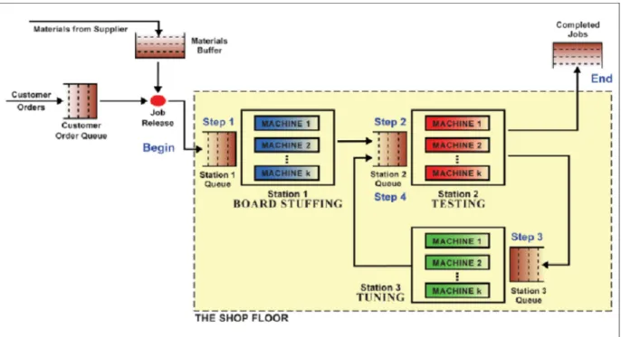
5.2 Littlefield Technologies

Introduction

Sam Wood and Sunil Kumar (Stanford’s Graduate School of Business) developed a web-based serious game, named Littlefield Technologies (in short Littlefield), to address the challenges students face with topics of capacity and inventory and to combine these into an integrated set of knowledge and skills. They collaborated with Responsive Learning Technologies (Responsive.net) to provide their game to educational institutions. Responsive Learning Technologies now offers various online serious games that can be accessed via their website (e.g. sourcing game, venture capital game, beer game) with instructor notes and assessments. Littlefield Technologies is used in both graduate and undergraduate classes and already a thousand of students played the simulation (Responsive Learning Technologies, 2014).