Definitions measurement procedures and composite walls – KLIMAPEDIA

Building Acoustics

Definitions, Measurement

Procedures and Composite Walls

1

Definitions, Measurement Procedures and Composite Walls

by L. Nederlof, J.J.M. Cauberg and M.J. Tenpierik

1.1

A brief introduction to the wave character of sound

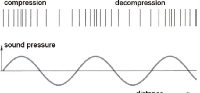
If a flat plate in air is moving periodically back and forth in the direction perpendicular to the plate, the air in front of the plate will consecutively be compressed and stretched (figure 1.1). This can be imagined as follows. If the plate moves to the right, the air to the right of the plate is compressed. This compressed air has a higher air pressure, as a result exhibiting a force in rightward direction on the air in front. As a result, the air in front of this compression zone starts to move and gets in turn compressed. If the plate moves to the left, the air on the right side still moves to the right resulting in a zone with lower pressure next to the plate. This in turn exerts a force in leftward direction on the air in front. This process continues as long as the plate vibrates. Because of the vibrating plate, thus, the air in front of the plate vibrates as well and this vibration is spreading through the air in front of the plate. The resulting wave is called a longitudinal wave because the vibration of the air particles is in the same direction as the movement of the wave itself. If the vibration frequency and amplitude of the plate are large enough, the wave can be

perceived as sound.

Figure 1.1 – Sound as a longitudinal wave with compression and decompression zones. From a physical perspective, two equilibrium mechanisms are at play:

• _{force equilibrium which makes the medium move;}

• _{the continuity principle which expresses the density of the vibrating medium.}

A comprehensive and formal derivation can be found in text books (Berkhout and Boone, 1995). Here, a somewhat different and simpler derivation of the wave equation will be presented.

Consider a thin pocket of air of 1 m2 _{with a thickness dx and mass rdx (figure 2). The air pressure on both}

sides of this pocket of air is set to p1 and p2 respectively. Both the pressure, p, and the particle velocity, v,

are a function of place and time: p=p(x,t) and v=v(x,t). If x and t vary with dx and dt respectively, then p and v generally vary according to

p p dp dx dt x t ∂ ∂ = + ∂ ∂ and dv v_xdx v_tdt ∂ ∂ = + ∂ ∂

For the movement of the air pocket under the influence of the pressure difference p2 – p1, it is important to

realise that this is a difference in momentary values. As a result, we can write

1 2 p p p dp dx x ∂ − = − = − ∂

Figure 1.2 – Physical model for a single-leaf wall for normally incident acoustic waves.

As long as dx is very small, the velocity of the air particles on both sides of the air pocket may be considered constant, or v dv dt t ∂ ≈ ∂

If we now apply Newton’s second law of motion (force equals mass times acceleration) to this air pocket of 1 m2_{, the following equation emerges:}

1 2 p dv v p p− = −∂_xdx=ρdx_dt ≈ρdx∂_t ∂ ∂ As a result, p v x ρ t ∂ _{= −} ∂ ∂ ∂ (1.1).

Regarding the continuity principle, we consider an air spring that has a length dx and of which both ends move over a distance u and u+du respectively. If we then apply Hooke’s law, we get

u p= −K ∂_x

∂ (1.2),

with

K = the compression modulus or dynamic modulus of elasticity [kg/(m∙s2_{) or Pa]}

∂_{u/∂x = the specific strain [-]}

By definition, v = ∂u/∂t. If we now differentiate equation (1.2) with respect to time, we as a result get

p _K v t x

∂ _{= −} ∂

∂ ∂ (1.3).

If we now differentiate equation (1.1) with respect to x and equation (1.3) with respect to t, combine both resulting equations and eliminate the combined term ∂2v/∂x∂t, we get the wave equation for sound:

2 2 2 2 p K p t ρ x ∂ ∂ = ∂ ∂ (1.4a). mass ρ∙dx p2 = p1 + ∂p/∂x dx p1 x-direction dx u u + du

Typically, this equation is written as 2 2 2 2 2 p _c p t x ∂ ₌ ∂ ∂ ∂ (1.4b).

In this equation, the constant c is the speed of the sound wave progressing through the medium

K

c= _{ρ (1.5).}

At room temperature, this speed equals approximately 343 m/s if the medium is air.

Because of its one-dimensional character, previous differential equation is only valid for so-called planar progressive waves. Another simplification involved in the derivation of this equation concerns the fact that we did not consider that compression of air irrevocably results in heat production caused by internal friction. A part of the (acoustic) energy that is transported by the wave is thus irreversibly converted into heat. As a result, the acoustic wave will slowly be dampened till (fortunately) the sound has decayed. Wave equation (1.4) has two periodic solutions corresponding to wave progression in positive and negative x-direction: ω±      = _ ± _= ⋅   max x i t c x p p t _c p e (1.6a), with

pmax = the pressure amplitude of the wave [Pa] c = the progression speed of the wave [m/s]

ω _{= the angular frequency with which the momentary sound pressure fluctuates. It relates to the}

sound frequency or tone via ω = 2πf [rad/s] Equation (1.6a) is sometimes also written as

(ω ± )

= _max⋅ i t kx

p p e (1.6b),

with

k = the wave number equal to ω_{/c [rad/m]}

If we differentiate equation (1.1) with respect to t and equation (1.3) with respect to x, combine both resulting equations and eliminate the combined term ∂2_{p/∂x∂t, we get another wave equation for sound:}

2 2 2 2 2 v _c v t x ∂ ₌ ∂ ∂ ∂ (1.7).

For the particle velocity, v, we thus get a solution similar to equation (1.6a): ω±      = _ ± _= ⋅   max x i t c x v v t _c v e (1.8). Characteristic to sound waves is that the progression direction of the sound wave coincides with the vibration direction of the air particles, or in others words a sound wave is a longitudinal wave.

At first, one would expect a phase difference between sound pressure and particle velocity. However, this is not the case since according to the equations pressure and particle velocity are correlated as

p=ρc v⋅ _(1.9),

with

ρ_c = the specific acoustic wave impedance. It is the product of density and wave velocity. For air at room temperature, it approximately equals 410 kg/(m2_∙s).

At a random position and time, the wave energy has two components: kinetic energy of the air particles and potential energy of the compressed air (spring). Using equations (1.5) and (1.9), we can write for the momentary energy per unit volume, i.e. for the energy density of the planar wave

2 2 2 2 1 1 2 2p p E ρv _{K c} ρ = + = (1.10).

Typically, the medium in which the sound waves progress is air. Other gases, liquids or solids can also act as medium, each have its own sound speed (c = K ρ/ ) and specific acoustic wave impedance ρ_{c. Table}

1.1 gives an overview of these properties for several ‘materials’.

The acoustic wave impedance plays among others a role at the transition of sound waves from one medium to another; and determines the degree of reflection at the interface. If air is the medium in which the sound waves progress, if the circumstances are adiabatic and if pressure variations are small, the compression modulus can be derived from the perfect gas law as

0 / p V

K c c p= ⋅ _(1.11),

with

p0 = the atmospheric pressure (1 atm. = 1.013·105 Pa)

cp = the specific heat at constant pressure [J/(kg∙K)]

cV = the specific heat at constant volume [J/(kg∙K)]; cp / cV ≈ 1.4 for air

material ρ _[kg/m3_] K or E_{dyn [N/m}2_] c [m/s] air 1.2 14·104 ₃₄₀ cork 250 62·109 ₄₉₈ brick 2000 25·109 ₃₅₃₆ concrete K300 2400 35·109 ₃₈₁₉ concrete K225 2200 20·109 ₃₀₁₅

lightweight concrete (Holith) 1700 28·109 ₄₀₅₈

floatstone 1000 5·109 ₂₂₃₆ gypsum board 800 4·109 ₂₂₃₆ gypsum 700 7·109 ₃₁₆₂ steel 7800 210·109 ₅₁₈₉ aluminium 2800 70·109 ₅₀₀₀ lead 12200 17·109 ₁₁₈₀ float glass 2500 70·109 ₅₂₉₂ pine wood 470 10·109 ₄₆₁₃ red meranti 600 10·109 ₄₀₈₂

plywood oregon pine 580 12·109 ₄₅₄₉

chipboard 650 3·109 ₂₁₄₈

hardboard (normal) 1000 4·109 ₂₀₀₀

As said previously, the acoustic wave differential equation and its solution did not include the damping effect of air. In order to include this damping mechanism, equation (1.1) needs to be extended with an additional term representing damping losses. We will suffice here by showing how this addition modifies equation (1.6a) by adding a term causing the wave amplitude to decrease exponentially with distance:

α ω   ±   −     = _ ± _= ⋅ ⋅   max x i t c x x p p t p e e c (1.12), with

α = the damping or attenuation coefficient, having an order of magnitude of 10-3 _[1/m]

Air damping or air absorption is an important element in sound transmission but becomes only apparent at large distances. As a result, it is typically only considered in the acoustics of big spaces and when dealing with traffic noise. This also implies that in a small region around a point of the sound field the term _⋅ −α

max x

p e is constant, as a consequence of which the simplified wave model is an adequate approximation. For a molecular treatment of how the damping coefficient depends on frequency, temperature, viscosity and humidity, we refer to (Berkhout and Boone, 1995). Figure 1.3 presents some values of the damping coefficient as function of temperature, relative humidity and frequency.

Despite the simplifications made in this section, we can still conclude that the transmission of sound in a free field is influenced by air temperature, atmospheric pressure, relative humidity, presence of air layers with different temperature (inversion) and wind.

1.2

General definitions

1.2.1 Sound insulation (transmission loss), sound proofing and sound reduction

Sound insulation (transmission loss) is defined as the amount of sound energy that is blocked by a certain construction. This is a specific definition and is mathematically defined in section 1.2.4.

Sound proofing and sound reduction are terms often used in everyday language but are not clearly defined. As a result, the use of these terms may lead to misunderstandings.

Typically, sound proofing involves all measures that are taken in order to reduce the sound levels in a room to acceptable levels. This can thus be improving the sound insulation of facades or interior walls but also adding sound absorption in a room.

Sound reduction is a container term that describes damping, a weakening of sound, or a level difference. It is sometimes mistakenly misinterpreted as a being equal to sound insulation. As we will see, sound reduction does not equal sound insulation.

1.2.2 Airborne and structure-borne sound insulation (impact sound insulation)

When dealing with sound insulation we distinguish between airborne sound insulation on the one hand and structure-borne sound insulation or impact sound insulation on the other hand.

Airborne sound insulation relates to the insulation against sound waves in air that are generated by an acoustic source. The construction between two rooms is thus excited by an acoustic wave in air. In one room a person is for instance talking or playing music and in another (adjacent) room this sound needs to be limited.

Structure-borne sound insulation deals with the insulation against vibrational waves inside materials directly caused by a mechanical source. The construction between two rooms is thus excited by a mechanical source. In this case the vibrational waves are introduced into the material or structure by for instance a washing machine, a walking person, a toilet, water pipes, etc. Also in this case the noise in another (adjacent) room needs to be limited.

Both the terms airborne sound insulation and structure-borne sound insulation are specific terms which are mathematically defined, as we will see later.

1.2.3 Direct, flanking and indirect sound transmission

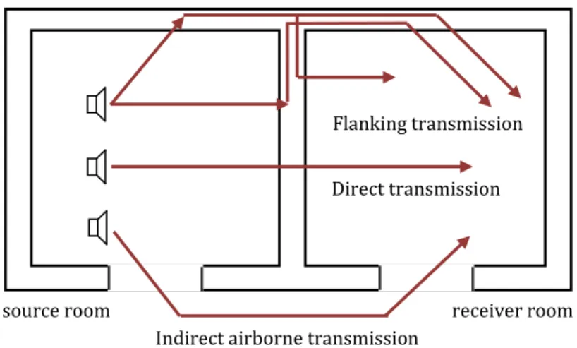
Sound can travel from one room or space to another via different transmission paths. These types of sound transmission are called direct (airborne) transmission, flanking transmission and indirect airborne transmission (Figure 1.4).

Direct sound transmission involves the sound transmission directly through the partition wall between the two rooms.

In case of flanking transmission, sound waves inside the source room create bending waves inside flanking walls, i.e. side walls, floor and ceiling, and/or the direct partition wall that travel via the junction towards other walls surrounding the receiver room. These walls surrounding the receiver room emit energy thus creating sound waves inside the receiver room.

Indirect airborne sound transmission finally is the transmission of sound via for instance air cavities, suspended ceilings and hallways.

Figure 1.4 – Direct, flanking and indirect transmission paths of sound from one room to another.

1.3

Some relevant basic acoustic properties

1.3.1 Sound speed (in air and in materials)

Sound in air is a longitudinal wave, i.e. a wave for which the vibration direction of the air molecules is equal to the direction in which the wave progresses. The speed with which the wave progresses is called the wave speed or velocity. For a sound wave in air this speed, cair, equals

ρ = air air air K c (1.13), in which

Kair = the dynamic compression modulus of air [N/m2] equal to approximately 1.4 p0

ρair = the density (≈ 1.21 kg/m3 for air at 20oC).

In dry air at 20o_{C and at standard atmospheric pressure, the speed of sound approximately equals 343}

m/s. As the density and the compression modulus of air depend on temperature, also the speed of sound in air depends on temperature according to the following equation that assumes air to be an ideal gas

ϑ =_{331.3 1}+ 273.15 air c (1.14), with

θ = the air temperature in degree Celsius [o_C].

A sound wave cannot only progress in air, it can also move as a longitudinal wave inside solids. The longitudinal speed of sound inside solid materials can be found from

(

)

(

)(

)

E = is the Young’s modulus of the material [N/m2_]

ρ _{= the density of the material [kg/m}3_]

ν = the Poisson’s ratio [-].

Table 1.1 gives an overview of the speed of sound in several materials.

source room receiver room

Flanking transmission

Direct transmission

1.3.2 Sound pressure, sound power and sound intensity

Sound causes pressure fluctuations around the atmospheric pressure in air. If these pressure fluctuations are large enough, i.e. if these have a large enough amplitude, and if the frequency of these fluctuations is right, they can be perceived by our ears as sound. Two aspects of these fluctuations are observed, the amplitude, which represents the loudness of the sound, and the frequency, which represents the pitch of the sound.

If a person hears a pure sinusoidal tone for a while, he/she perceives the loudness of this tone as constant. This means that we cannot take the instantaneous pressure, p, as a measure for loudness; our ears do not perceive the fluctuation of this pressure. Also the average pressure cannot be used as a measure for loudness for the average pressure of a sinusoidal fluctuation is zero. For physiological and energetic reasons, therefore, an effective pressure was introduced, peff. This effective pressure is the square root of

the time-average squared sound pressure

( )

∫

Young healthy people can just still hear an effective sound pressure of 20 µPa (=20·10-6 _{Pa) at 1000 Hz.}

This pressure is called the hearing threshold, p0. The pain threshold is reached for an effective pressure of

200 Pa. At that pressure the hearing organ can be damaged.

It is common knowledge that the sound levels at a distance from a source are lower than close-by the source. It is therefore useful to introduce a parameter that characterises the acoustic strength of a sound source. This parameter is called sound power, W [W]. It reflects the acoustic energy that is produced by the source.

The further the sound wave gets from the source, the bigger the area of the wave front becomes. In an ideal case the total acoustic power of the sound wave remains constant. However, because it is spread out over a larger area, the acoustic power per m2 _{wave area decreases. This acoustic power per m}2 _{is called}

the acoustic intensity, I [W/m2_{]. Acoustic intensity thus is the acoustic energy that per unit of time ‘falls’}

onto a unit of area.

In case of a spherically progressing sound wave, i.e. a point source in a free field, the acoustic energy at distance r from the source equals

π = ₂ 4 W I r (1.17).

In case of a line sound source with length l, acoustic power is typically provided as a power per meter [W/m]. The sound intensity in a free field at distance r then becomes

π π

= =

2 2

Wl W

I _{rl r} (1.18).

In practise, however, acoustic sources are placed on the floor. If we assume that this floor is perfectly reflecting the sound, the acoustic wave is progressing in the form of half a sphere or half a cylinder. Instead of 4πr2 _{and 2πrl the surfaces through which the energy passes then become 2πr}2 _{and πrl}

For a plane progressing wave in the direction of wave progression, the intensity equals ρ = eff2 air air p I c (1.19),

Whereas for a diffuse sound field, it equals

ρ

= 2

4 _{air air}eff

p I

c (1.20).

1.3.3 Sound levels (sound pressure, power and intensity levels)

Our ears are sensitive to a wide range of sound pressures, powers and intensity. For example, the hearing threshold for effective sound pressure at 1000 Hz equals 20 µPa whereas the pain threshold lies around 200 Pa, which is 7 orders of magnitude higher. It is difficult to work with numbers that have such big differences. Therefore, a new parameter that is based on a logarithmic scale was introduced. Related to sound pressure, this parameter is called sound pressure level, Lp or SPL [dB]. It is defined as

  = _ _   2 2 0 10log eff p p L p (1.21), with

p0 = a reference sound pressure level which equals the hearing threshold at 1000 Hz (20 µPa).

Because Lp reflects the ratio of peff to p0, the reference pressure should always be mentioned. It is written

as Lp = x dB re. 20 µPa. The unit of sound level is the decibel. This name is derived from deci-Bell with

‘deci’ denoting the factor 10 and Bell the name of the person who the unit is named after. If the sound pressure level is corrected for our ear sensitivity according to the A-weighting curve, the unit is dB(A). As said, the hearing threshold and pain threshold at 1000 Hz for a normal youngster lie near 20 µPa and 200 Pa respectively. This means that the respective sound pressure levels equal

(

)

(

)

( )

( )

(

)

(

)

( )

10log 10log 10 10 14 10log 10 140

20 10 p

L dB pain threshold.

Table 1.2 provides an overview of sound pressure levels of several common sounds.

Besides sound pressure level, also logarithmic parameters have been introduced for sound power and sound intensity. They are defined as

  = _ _  0 10log W W L W (1.22),   =  _{ }  0 10log I I L I (1.23),

Type of sound Lp [dB]

Hearing threshold 0

The stirring of leaves 20

Whispering at 1 m distance 40

Normal conversation at 1 m distance 60

Noise at 50 m distance from a busy highway 70

Alarm clock at 0.7 m distance 80

Heavy lorry at 15 m distance 90

Horn of a car close-by 100

Discotheque 110

Ascending air plane on the runway at 70 m distance 120

Pain threshold (average) 140

Right in front of the speakers at a rock concert 150 Table 1.2 – sound pressure level of common sounds in which

LW = sound power level [dB]

W0 = a reference sound power set to 10-12 W LI = sound intensity level [dB]

I0 = a reference sound intensity set to 10-12 W/m2.

The values of W0 and I0 were not chosen arbitrarily. For a planar progressing wave, sound intensity equals peff2 / (ρaircair). The reference intensity can this be found from p02/(ρaircair) = 20·10-6/(1.21·343) ≈ 10-12

W/m2_{. That means that also the sound intensity level starts at 0 dB. From this we can also conclude that}

for a plane progressive wave the sound intensity level on a surface perpendicular to the progression direction of the wave equals the sound pressure level because

ρ ρ       =  _{ }= _ _= _ _=       2 2 2 2 0 0 0 /

10log 10log 10log

/

eff air air eff

I p air air p c p I L L I p c p

Also between sound power level and sound pressure level a relation can be found (valid at a certain distance from the source); for both a point source and a line source.

π π − π       =  _{ }=  _⋅ = _ _= −       2 2 12 2 0 0 1

10log 10log 10log 10log(4 )

4 10 4

I I W W W

L L r

I r W r

At a distance from the source, we can thus also write π

= −_10log(4 2₎

p W

L L r point source in a free field (1.24).

As can be seen from this equation, if we double the distance r from the source, the sound pressure drops with 10log(22_{) = 6 dB. Or for a point source in a free field the sound pressure level drops with 6 dB for}

every doubling of distance.

Similarly, for a line source we can derive π

= _{−10log(2 )}

p W

L L r line source in a free field (1.25).

1.3.4 Reverberation time

The reverberation time is a property of a room that reflects the amount of reverberation, i.e. the slow decay of the late sound reflections. In the early 1900s, Wallace Clement Sabine defined the reverberation time as the time that elapses from the moment a sound source is switched off till the moment the sound has decayed by 60 dB. The longer the reverberation time of a room is, the more reverberant the room thus is. According to Sabine, reverberation time can be calculated from

=55.3 ≈1 6 air V V T c A A (1.26), with

V = the volume of the space [m3_]

A = the total sound absorption inside the space [m2 _sabin].

The total sound absorption is derived from the surfaces with present in the room and the absorption coefficient of each surface as

α = =

∑

α = the absorption coefficient of a surface [-] S = the surface area of a surface [m2_]. 1.3.5 Frequency and wave length

The frequency, f, of a sound wave denotes the number of sound pressure fluctuations per second. Frequency and amplitude are the two properties of a sound wave that our ears use to characterise the sound. Where amplitude relates to the perception of loudness, frequency relates to the perception of pitch. Frequency is the reciprocal value of period or vibration time, Tp, that reflects the time needed for one

fluctuation to take place

= 1 p

f

T (1.28).

Wave length, λ, is the distance between two consecutive points that have identical state, i.e. that are in phase. In case of a transversal wave, it is the distance between two maxima or minima; in case of a longitudinal wave, it is the distance between two zones with maximum pressure or with minimum pressure (Figure 1.5). Wave length and frequency are coupled by the speed of the wave as

λ= /c f (1.29).

Figure 1.6 – Reflection, absorption and transmission of sound.

1. 4

Airborne sound insulation: a mathematical definition

When a sound wave hits a wall, part of it is reflected, part of it absorbed in or by the wall and part of it transmitted through the wall (Figure 1.6). On the front side of the wall there is a sound field with sound power level LW;i while at the back side of the wall a sound field results with sound power level LW;t. The

difference between the sound power level on the front and at the back side is defined as the airborne sound insulation of this wall, R [dB]:

; ;

0 0

10log i 10log t 10log i W i W t t W W W R L L W W W       = − = _{ }− _{ }= _{ }       (1.30a).

For constructions consisting of just one material, W = IS, with I [W/m2_{] the acoustic intensity and S [m}2_]

the surface area of the wall. As a result, equation (1.30a) can also be written as

10log i t I R I   =     (1.30b).

Based on intensities, we can now define an energy-transmission coefficient, t, as

t i I t I = _(1.31).

Combining equations (1.30) and (1.31) gives us the definition of airborne sound insulation as   = _{ }= −   1 10log 10log( ) R t t (1.32).

This definition does neither include information on the direction of the sound nor on its frequency. That means that this definition can be used for normal sound incidence, oblique sound incidence or random sound incidence as well as for each frequency. In principal the airborne insulation of building

constructions or parts of building construction depends on frequency. For each frequency this sound insulation must thus be determined. It is here important to realise that SOUND INSULATION is NOT the same as SOUND ABSORPTION.

incident energy Wi reflected energy Wr transmitted energy Wt absorbed energy Wa 0 10 log i Wi W L W   = ⋅     0 10 log t Wt W L W   = ⋅ _{ }  

Figure 1.7 – Surface mass and sound insulation.

As we will see in chapter 3, mass, or more precisely surface mass (kg/m2_{), is an important parameter that}

influences the airborne sound insulation. This can be explained as follows. As explained, a sound wave is a longitudinal wave that causes air to have zones with higher pressure and zones with lower pressure. If such a wave impacts on a wall, it exerts consecutively a pushing and a pulling force on this wall causing this wall to move forward and backward; the wall vibrates. This wall again causes the air on the other side to vibrate. Newton’s second law of motion describes that the change of the motion of a mass is directly proportional to the force that is exerted on this mass, or =F ma(force = mass times acceleration). So, the fluctuating pressure difference over the wall causes a fluctuating acceleration of this wall with mass acting as a proportionality factor. This means that the higher the mass is, the smaller the

acceleration is and thus the smaller the vibration amplitude of the wall is; it so to speak more difficult to have a wall with high mass vibrate than to have a wall with low weight vibrate. This smaller vibration amplitude also results in a lower sound pressure on the backside of the wall. Or in other words, a wall with high mass lets less sound trough and thus has a higher airborne sound insulation than a wall with low mass. Something similar holds for the number of vibrations per second, or the frequency. High frequent sound will be less easily transmitted through a wall than low frequent sound.

For example, a concrete wall of 10 cm thick lets at 500 Hz and for normal incidence of sound waves only a fraction of 0.000001 of the sound energy pass through. This means that for these conditions it has an airborne sound insulation value of -10log(0.000001)=60 dB. 3 mm glass on the other hand for the same conditions lets a fraction of approximately 0.001 of the sound energy pass through. This means it has an airborne sound insulation of 30 dB. Figure 1.7 shows this difference.

1.5

Composite walls

1.5.1 General description

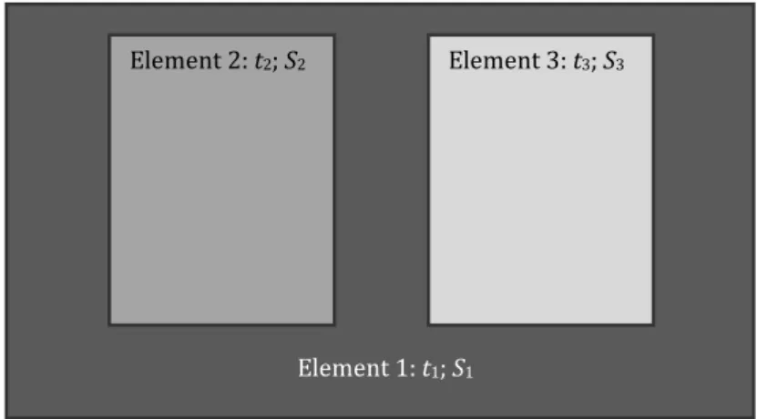
The definition of the airborne sound insulation in section 1.2.4 was said to be applicable when a wall, façade or partition wall only consists of one construction element with transmission coefficient t and surface area S. Very often building constructions are made of several construction elements together making a complete wall or façade (Figure 1.8), for instance a glass window inside a brick wall. Each of these elements has its own airborne sound insulation. Since this building construction is made of several elements or components, we must define an average transmission coefficient for this construction. This average transmission coefficient is defined as

1 1 2 2 1 1 2 1 ... ... n i i n n i n n i i t S t S t S t S t S S S S = = + + + = = + + +

∑

∑

Figure 1.8 – Building construction built up from several elements

Using this definition of average transmission coefficient and equation (1.32), the airborne sound insulation of a composite wall can be defined

( )

Combining this equation with equation (1.33) and with ti = 10-Ri/10, we can re-write this into

(

)

∑

∑

1.5.2 Introduction to air gaps and ventilation grills

As a very rough estimate, an air gap can be included in equation (1.34b) as an element with certain surface area S and airborne sound insulation of 0 dB. If there is only one construction element with a small gap of surface area S, we can then write

1/10 /10 1/10

1 1

1 1

10 10 10

10log R gap Rgap 10log R gap

res gap gap S S S S R _{S S S S} − − −  ⋅ + ⋅   ⋅ +  = − _ _= − _ _ + _ + _   (1.35).

If we now assume that the airborne sound insulation of the wall, in which the gap appears, has much higher sound insulation compared to the gap itself, we can see that because of the gap a certain maximum sound insulation value exist. This maximum can be found if the airborne sound insulation of the wall, R1,

approaches infinity, or 1 1 /10 1 max 1 1 10

lim 10log R gap 10log gap

R _{gap gap} S S S R S S S S − →∞   ⋅ +    = − _ _= − _ _ + +        (1.36).

This equation tells us that. If a gap exists in a wall, the airborne sound insulation of this composite wall can never be higher than the value calculated with equation (1.36). As can be seen from figure 1.10, a

Element 1: t1; S1

Figure 1.9 – the combined airborne sound insulation of a Figure 1.10 – the combined airborne sound

composite wall with surface S consisting of a well-insulating insulation of a wall with an air gap as function of the part with surface S1 and R1 and a worse insulating part with gap size. The numbers along the lines denote the

air-surface S2 and R2. The numbers along the lines denote S2/S. borne sound insulation of the wall itself, R1.

small gap already results in a sharp decrease of the airborne sound insulation of the composite wall, particularly when R1 is big. This means that air gaps need to be prevented or closed as much as possible in

order to achieve a high airborne sound insulation.

Until now it was assumed that the airborne sound insulation of a gap equals 0 dB. This, however, is not entirely true. Therefore, equation (1.34b) is typically extended to include both ventilation openings and seams. The effect of gaps and seams is then represented by a K for which values are determined from measurements. Equation (1.34b) is then modified as

(

)

∑

Dn = the normalised sound level difference of a ventilation provision, normalised to 10 m2 sabin [dB] K = the gap term

As can be seen, this equation comprises of three part: a part that expresses the sound insulation and surface area of closed elements, a part that reflects the effect of ventilation provisions and a part that expresses the effect of joints and seams.

For most windows, the window frame can generally be neglected and thus its area can be added to the glass itself. The sound insulation of window frames is generally in the same order of magnitude as the glass. However, in case of high acoustic performance glass, i.e. an airborne sound insulation of more than 35 dB(A), the frames should be considered separately in the calculation. Certain standardized calculation methods, like the GGG calculation method in the Netherlands, require window frames and similar façade elements always to be included separately.

Many simple ventilation provisions and cantilever windows have a very low sound insulation value. They can thus lead to a significant reduction of the sound insulation of a whole façade. Particularly where the outdoor noise levels are high, either mechanical ventilation should be chosen or provisions for natural ventilation with better sound insulation should be used. Such ventilation provisions are baffle filters. A baffle filter is a ventilation box that contains sound absorbing material. The sound that is transmitted through this baffle filter is to a large extent absorbed by the absorption material, as a result increasing the sound insulation of the provision for natural ventilation.

Sgap/(Sgap+S1) [-] R res [d B] 0 0.2 0.4 0.6 0 10 20 30 5 dB 15 dB 50 dB R1-R2 [dB] R1 - R [d B] 10 15 20 0 10 20 30 1 5 25 30 0.3 0.1 0.03 0.01 0.003 0.001

The absorption material inside the baffle filter also increases the resistance the air flow encounters as a result reducing the maximum ventilation rate through this filter. Therefore, both the ventilation capacity of the baffle filter and its sound attenuation should be determined in a laboratory according to standards. The sound attenuation is then normalized onto a fictitious area of 10 m2_{. As can be seen from the equation,}

this 10 m2 _{is also used as surface area of the baffle filter instead of its real gross area. This real area is thus}

not included as area of the baffle filter in the calculation; however, it should be included when calculating the total surface area, Stot, of the whole façade.

When applying a provision for natural ventilation in a façade, always a balance needs to be found between the ventilation capacity and the sound attenuation. Generally, if the sound attenuation of the baffle filter increases the net ventilation that passes the filter decreases (expressed in dm3_{/s per meter}

baffle filter). Besides, if a longer baffle filter is installed, a higher ventilation rate can be achieved but at the same time the sound attenuation is reduced. The sound attenuation, or the normalized sound level

difference of the baffle filter, Dn, can be determined from

  = − _ _   ; ; ; 10log v vent n e n lab q D D C (1.38), in which

Dn;lab = the normalised sound level difference measured in a laboratory and normalised onto 10 m2

sabin [dB]

qv;vent = the required ventilation capacity [dm3/s]

C = the air flow pass-through measured in a laboratory [dm3_/s/m]

Gaps and seams can also lead to a strong reduction of the sound insulation of a façade. As can be seen from Figure 1.11, the sound insulation of a gap depends on the thickness and width of the gap. However, in standardized calculations it is assumed that the total length of all gaps and seams is related to the surface area of the façade. As a result, the dimensions of gaps and seams are not included in the calculation. Instead, the sound insulation is expressed as a factor K that includes the relation between gap/seam size and area. This K-term is strongly affected by the quality with which the gap and seam is treated in the design and building process. Also with gaps and seams the right balance should be found; in a façade that

Figure 1.11 – the effect of a slit with width, b, on the airborne sound insulation of a wall with thickness, dwall, of 75 mm;

values along the lines denote the width, b, of the gap.

gap b dwall f [Hz] R [d B] 250 500 1000 2000 10 20 30 40 50 0 mm 1 mm 3 mm 5 mm

Situation Gap term, K RA [dB]

Existing dwellings Facades

- without provisions 3·10-3 ₂₅

- single gap sealing 1·10-3 ₃₀

- double gap sealing and improved joint sealing 3·10-4 ₃₅

- special double gap sealing (remaining good joint sealing, two- or three-point clamp fixing, draught mouldings welded to corners, sound attenuator connection carefully sealed)

3·10-5 ₄₅

Roofs

- with gaps in roof boarding 1·10-3 ₃₀

- with gap-tight roof boarding 1·10-4 ₄₀

New dwellings Facades

- single gap sealing and good joint sealing 3·10-4 ₃₅

- double gap sealing and good joint sealing 1·10-4 ₄₀

- special double gap sealing (remaining good joint sealing, two- or three-point clamp fixing, draught mouldings welded to corners, sound attenuator connection carefully sealed)

1·10-5 ₅₀

Roofs

- with single scale roof elements < 30 kg/m2 _3·10-5 ₄₅

- other roof structures 3·10-6 ₅₅

Table 1.3 – Gap term values (van der Linden et al., 2006).

in itself has a poor sound insulation performance gaps and seams require less attention than gaps and seams in a façade with high sound insulation performance. Table 1.3 provides an overview of several gap terms. It is important to realize that both gaps and joints must be determined separately. And finally, it is important to realize that in some standardized calculation methods, like in the Dutch GGG calculation method, it is not allowed to work with these gap terms.

1.6

Lab and In-Situ Measurement Procedures

1.6.1 Lab measurements of the airborne sound insulation of building elements

According to equation (1.30b) sound insulation is defined using sound intensities (or sound powers). It is, however, very difficult to measure sound intensity. Therefore another method that used sound pressures was developed in order to measure the airborne sound insulation of construction elements. This has led to the normalised method for measuring the airborne sound insulation of building elements in a laboratory (EN-ISO 10140-2: 2010).

Because only the airborne sound insulation of the building element and not all kinds of flanking

transmission paths or indirect airborne transmission paths need to be measured, high requirements are in place for the test laboratories and the equipment used (EN-ISO 10140-2: 2010). An acoustics laboratory for measuring airborne sound insulation consists of two transmission chambers (Figure 1.12). A source room where noise, typically white noise, is produced and a receiver room. Between these two rooms there is an opening of specified dimensions where the building element can be mounted. For glazing elements the connection details are specified in the standard. Sound can now only reach the receiver room through the building element.

For the measurements it is important that the sound field in both the source and the receiver room is diffuse. This is ensured by the non-orthogonal placement of certain walls and ceiling and by additional reflectors inside the rooms.

Figure 1.12: Plan and cross-section of the sound transmission chambers at TUDelft.

The sound intensity of such a diffuse sound field can be found from equation (1.20). So, in the source room, the acoustic power, Ws, that impacts on the surface of the building element with area S equals

ρ = = 2 ; 4 eff s s s air air p W I S S c (1.39a), with

Ws the acoustic power onto the building element in the source room [W] Is the sound intensity in the diffuse sound field of the source room [W/m2] S the surface area of the building element to be measured [m2_]

peff;s2 the effective sound pressure in the source room [Pa]

ρaircair the specific acoustic impedance of air (≈410 kg/(m2·s)

The building element starts to vibrate because of the impacting sound power in the source room and gives off a sound power in the receiver room equal to Wr = t·Ws. This sound power Wr leads to a sound intensity Ir in the receiver room that depends on the amount of sound absorption in that room

ρ = = 2 ; 4 eff r r r r r air air p W I A A c (1.39b), with

Wr the acoustic power given off by the building element in the receiver room [W] Ir the sound intensity in the diffuse sound field of the receiver room [W/m2] Ar the total sound absorption in the receiver room [m2 sabin]

peff;r2 the effective sound pressure in the receiver room [Pa]

If we substitute these sound powers in the definition of airborne sound insulation (eq. (1.30)), we obtain

ρ ρ         _{ }   _{   }   = _ _= _{ }= _{ }= _{ }                 2 2 ; ; 2 2 ; 0 2 2 2 ; ; ; 2 0 4

10log 10log 10log 10log

4

eff s eff s

eff s

s air air

r eff r eff r r eff r

r r air air p p S S _{p S} W c p R W p p A p A A c p

or identically,   = − + _ _   ; ; 10log p s p r r S R L L A (1.40). with

Lp;s the sound pressure level of the diffuse sound field in the source room [dB] Lp;r the sound pressure level of the diffuse sound field in the receiver room [dB].

The airborne sound insulation can now be determined if the sound pressure level in the source and the receiver room are measured and the dimensions of the building element and the sound absorption in the receiver room are known. This sound absorption in the receiver room can be found from measuring the reverberation time of the receiver room and applying Sabine’s reverberation time equation (1.26)

= 55.3 air

V A

c T (1.41).

It is important to realise that R is a construction property that only depends on the materials built-up or layering of the building element. It does not depend on contextual factors like size of the building element or sound absorption in the receiver room. It means that the airborne sound insulation should not change if that building element is measured in a different laboratory (within measurement uncertainties). This is reflected by the third term in equation (1.41). If S or Ar changes also Lp;r changes as a result of which R remains the

same; if S doubles, 10log(S/Ar) becomes 3 dB but also the amount of sound energy passing through the

building element doubles as a result of which Lp;r increases with 3 dB; something similar happens if Ar

changes.

The airborne sound insulation in a laboratory is typically measured in the third octave bands ranging from 100 Hz to 3150 Hz or even up to 5000 Hz. Sometimes also the third octaves with mid frequencies of 50, 63 and 80 Hz are measured. However, most sound transmission chambers are too small for accurately measuring these low frequencies for it is difficult to realise good diffuse sound fields for these frequencies in small rooms. A diffuse sound field in a room occurs if there are many eigenfrequencies (modes) at the particular frequency band. If an eigenfrequency is excited, standing waves occur inside a room. Such a standing wave causes nodes and antinodes, i.e large local differences in sound pressure level. If in a frequency band many modes exist, many standing waves overlap and the sound field is ‘smoothened’ resulting in a more uniform sound pressure level field. The number of eigenfrequenties in a room, N, among others depends on room size and frequency as (Heckl and Müller, 2004)

π ∆ ≈_{4 3} air f f N V c (1.42), in which

V = the volume of the room [m3_]

f = the mid frequency of the frequency band [Hz]

∆_{f = the bandwidth of the frequency band, i.e. the difference between the highest and the lowest} frequency of that band [Hz].

As can be seen from this equation, the number of eigenfrequencies is small for the combination of a small room with low frequency band and narrow frequency bandwidth. This means that in that case there is little overlap of standing waves and a non-uniform non-diffuse sound field.

1.6.2 In-situ measurements of the sound insulation between two rooms

When looking at the sound insulation between two rooms, we are interested in the amount of sound that is transmitted from the room with the source to the room with the receiver. Contrary to the laboratory case, in practice there are more transmission paths than just through the partition wall. Besides this direct transmission, we have to deal with flanking sound transmission, indirect airborne transmission and transmission through leaks and seams. All these transmission paths are reflected in the final result of the measurement.

The sound pressure level in the receiver room is determined by • _{the acoustic power of the sound source in the source room}

• _{the resulting sound distribution inside the source room: a diffuse sound field is assumed} • _{the sound transmission through walls, floors, ceilings, etc.}

• _{the resulting sound distribution inside the receiver room: again a diffuse sound field is assumed} The sound reduction from one room to another can be determined from measurements according to normalised methods (NEN5077+C3: 2012 for dwellings for instance). A sound source in the source room produces noise containing the octave bands from 125 Hz to 2000 Hz. In both the source and the receiver room, the sound pressure level is typically measured for the octave bands with mid frequencies from 125 to 2000 Hz. These sound pressure levels need to be a spatial and temporal average of the room. Next, the difference between both sound pressure levels is calculated for each of these octave bands and normalised to a standardised furnishing of the room

  = − + _ _   ; ; 0 10log r nT p s p r T D L L T (1.43), in which

DnT = the normalised sound level difference between the source and the receiver room [dB] Tr = the average reverberation time of the receiver room [s]

T0 = a reference reverberation time of the receiver room (0.5 s for dwellings; 0.8 s for other

buildings)

Contrary to the laboratory-based airborne sound insulation R, DnT does depend on contextual factors. For

characterising the sound insulation in practice this is also needed because the actual sound pressure level in the receiver room does depend on the size of the partition wall and the furnishing of the receiver room. In the past, sometimes equation (1.40) was used to determine the sound insulation between two rooms in practice. The resulting value was denoted with R’ to make a distinction with the laboratory-based R. Because of the correction term 10log(S/Ar), R’ is independent of contextual factors like the surface area of

the partition wall and the sound absorption in the receiver room. In order to make R’ context-dependent it can be recalculated into DnT by

  = + _ _  0  ' 10log 6 nT V D R T S (1.44).

If there is only direct sound transmission through the partition wall, then R’ equals R. We may then conclude that a high sound level difference between source and receiver room, DnT, can be obtained for

• _{high sound insulation of the partition wall and high sound insulation against flanking and indirect} airborne transmission,

• _{for small surface area of the partition wall between both rooms and} • _{for high total sound absorption in the receiver room.}

1.7

Literature

Boone, M.M., D. de Vries and A.J. Berkhout (1995), Geluidbeheersing / Sound control, lecture notes c36d, Delft University of Technology, Delft.

EN-ISO 10140-2: 2010, Acoustics – Laboratory measurement of sound insulation of building elements – Part 2: Measurement of airborne sound insulation, CEN, Brussels.

EN-ISO 10140-5: 2010, Acoustics – Laboratory measurement of sound insulation of building elements – Part 5: Requirements for test facilities and equipment, CEN, Brussels.

Heckl, M. and H.A. Müller (2004), Taschenbuch der technischen Akustik, 3rd edition, Springer Verlang, Berlin.

Linden, A.C. van der et al. (2006), Bouwfysica, ThiemeMeulenhoff, Amersfoort.

Martin, H.J. (2007), Geluidisolatie, lecture notes for the course Acoustics 7S510, Eindhoven University of Technology, Eindhoven.

Nederlof, L. and Cauberg, J.J.M. (2005), “Golfkarakter van geluid”, Kennisbank Bouwfysica Module A1, Stichting Kennisbank Bouwfysica.

NEN5077+c3: 2012, Geluidwering in gebouwen – Bepalingsmethoden voor de grootheden voor geluidwering van uitwendige scheidingsconstructies, luchtgeluidisolatie, contactgeluidisolatie, geluidniveaus veroorzaakt door installaties en nagalmtijd, Nederlands Normalisatie Instituut, Delft.