Automatic analysis of cerebral sulci in ultrasound images

Academic year 2019-2020

Master of Science in de industriële wetenschappen: elektronica-ICT Master's dissertation submitted in order to obtain the academic degree of

Supervisors: Dr. David Van Hamme, Dr. Paul Govaert (ZNA Middelheim)

Academic year 2019-2020

Master of Science in de industriële wetenschappen: elektronica-ICT Master's dissertation submitted in order to obtain the academic degree of

Supervisors: Dr. David Van Hamme, Dr. Paul Govaert (ZNA Middelheim)

Preamble concerning COVID-19

During this study a global pandemic is broken out. This pandemic is all due to a virus called SARS-CoV-2 that is crazy spreadable. This virus causes the horrible coronavirus disease 2019, better known as COVID-19. It first broke out at the end of 2019 in Wuhan (China) but spread during this study to everywhere around the globe. Certainly Belgium, where this study takes place, isn’t saved from the virus. This disease already caused only in Belgium by August 2020 almost 10.000 deaths with over 70.000 confirmed cases. This led to a national lockdown. This means that no people were allowed to leave their homes for non-essential businesses.

This study isn’t touched hard by this lock-down, but it does had it’s impact in small ways. There was normally planned to have more feedback moments with my promotors dr. Van Hamme and dr. Govaert, who is specialised in analysing ultrasounds of the brains of preterm babies. There were meetings online, but these were not ideal. This is all led to a more independent study, but this is just a small level drawback.

Preface

This Master’s thesis has been written as a final piece to obtain the academic degree of Master of Science in Electronics and ICT Engineering technology at the University of Ghent, Belgium.

I would like to thank some people who made it possible to successfully complete this mater’s thesis. First, I would like to thank my promotor dr. David Van Hamme for his specific guidance, advice, time and the opportunity to do a study about this topic.

Secondly, dr. Paul Govaert from ZNA Middelheim deserves a special thanks. Dr. Govaert is specialised in the medical part of this study containing analysing the brains of a preterm baby. In this way, he gave certain amounts of his time to guide me and give a basic understanding how to read an ultrasound of the cortex at that stage of age. He also provided the whole dataset that was needed to start this study.

Finally, I would also like to thank the whole Image Processing and Interpretation (IPI) research group of the department Telecommunications and Information Processing (TELIN) of the Faculty of Engineering (FirW) at Ghent University. At multiple occasions they took the time to listen to my presentations about the progress of this study and gave me advice to come to a better overall research.

Admission to loan

The author gives permission to make this master dissertation available for consultation and to copy parts of this master dissertation for personal use. In all cases of other use, the copyright terms have to be respected, in particular with regard to the obligation to state explicitly the source when quoting results from this master dissertation.

Abstract

Medical imaging is a very time consuming task for doctors and in the latest trends, the demand for them still growing. This could lead to a shortage of trained doctors to take and analayse them. That’s why it is important that there are more studies dedicated to automatically analysing med-ical images.

In this master’s dissertation a tool is proposed to analyse the sulci of a preterm baby in an ul-trasound image. This will be done by building a pixel classifier that detects if a pixel belongs to a sulcus or not. There are multiple models with different algorithms and features trained on a dataset of around 50 ultrasounds of clear sulci patterns and tested with a set of 25 ultrasounds. The dataset images exist of DICOM files. For this reason, an implementation is added to read some of the important DICOM attributes such as the name of the patient, the age of the patient, etc. The features used are based on the edge detection techniques difference of Gaussian and Laplacian of Gaussian and the ridge detection based on Sato’s filter, Frangi’s filter, Meijerings filter and a hybrid Hessian filter. To compare the models multiple 5-fold cross validations are done on the training data and the testing data.

After the pixels are classified in to sulcus pixels or background ones, some analysing metrics are proposed. These are based on the skeletonised version of the labels of sulci. The metrics developed are a tortuosity level of the whole sulcus, the length of the root branch and a depth analysing graph that looks at the intensity values of an intersection of a sulcus.

To make this study available for testing, a GUI and web application is built. The GUI is more in-tended for usage during this study and not really for deployment, but it does have some advantages compared to the web tool.

Abstract— In this study, a tool is proposed to analyse the sulci

of a preterm baby in an ultrasound image. This will be done by building a pixel classifier that detects if a pixel belongs to a sulcus or not. There are multiple models with different algorithms and features tested on a dataset of around 50 ultrasounds of clear patterns of sulci. The dataset images exists of DICOM files. For this reason, an implementation is added to read some of the important DICOM attributes such as the name of the patient, the age of the patient, etc. The features used are based on the edge detection and ridge detection. The edge detection techniques are difference of Gaussian and Laplacian of Gaussian and the ridge detection are based on Sato’s filter, Frangi’s filter, Meijerings filter and a hybrid Hessian filter. There are also some sulcus analysing metrics proposed. These are based on the skeletonised version of the labels of the sulci. The metrics developed are a tortuosity level of the whole sulcus, the length of the root branch and a depth analysing graph that looks at the intensity values of an intersection of a sulcus. To make this study available for testing, a GUI and web application is built.

Index Terms—Gyrification, Sulci, Gyri, Computer vision,

Ultrasound images, Random forest, Skeleton Analysis, Webtool

I. INTRODUCTION

EDICAL imaging is a very time consuming task for doctors and by looking at the latest trends, the importance of them still growing. This could lead to a shortage of trained doctors to take and alayse them. That’s why it is important that there are more studies dedicated to automatically analysing medical images.

This study is dedicated to automatically analyse cerebral sulci of preterm babies in ultrasound images. The sulci are the grooves in a human brain and the development of them are crucial for our intellectual level. These start to form during pregnancy and develop throughout our whole life. This process is called gyrification. Sulci are always paired with gyri that are the ridges of a human brain. It is important to analyse these with preterm babies because the main part of the gyrification process takes place during the third trimester of pregnancy. This is the stage where preterm babies are born. If there are some serious deviations in the gyrification process detected at that stage, doctors could still try to help the infant.

It’s also important to notice that the images used in this study to analyse the sulci of a preterm baby are ultrasounds. An

ultrasound has some disadvantages over other medical imaging techniques, but for this study it has some handy advantages. The main disadvantage is that a basic understanding is needed of from which orientation the image is taken because it doesn’t represent the whole brain in one image. It also has some problems with noise. A major advantage of ultrasounds in this study is that the doctor who is taking them, can easily adopt to the movement of a preterm baby. This is important because some imaging techniques demand that the patient needs to lay perfectly still for a certain amount of time and this is very hard for a baby of that age. This is mentioned because this isn’t the first study that dedicates it’s time to try to automatically analyse cerebral sulci. One of the most important studies on this subject is done by the medical school of Harvard University. This research led to a matric that maps very good to the gestational age (GA) of a brain. This metric is called the Gyrification Index (GI) and it quantifies the amount of cortex within the folds of the sulci compared to the amount that is visible on the outer part of the brain. It also looks at local patterns of GI around sulcal pits. These are the deepest local regions of sulci because of the early forming of the first cortical folds. [1, 2]

II. DEVELOPMENT OF THE CEREBRAL CORTEX

The cerebral cortex is the outer layer of brain tissue. It exists of two almost symmetric hemispheres, which are separated by the longitudinal fissure. The process of gyrification causes the cortex to be folded in ridges, called gyri, and grooves, called sulci. These are formed so that the outer surface area increases. In this way more cognitive power is available to a human being. The locations of the gyri and sulci are not random but form a regular pattern. This causes a functional organization of the brain. There are four main regions called lobes. A visualisation is given in Figure 1. The first lobe is called the frontal lobe because it’s located at the front of each hemisphere. In this region most of the voluntary movement is processed. The second lobe is named the parietal lobe. This one lies behind the frontal lobe after the central sulcus. The parietal lobe mainly focuses on sensory information such as navigation and touch. The occipital lobe is located at the lower back of the human brain and processes mainly vision. The temporal lobe, at last, lies under the lateral sulcus that runs at the lower ends of the frontal and parietal lobes. The temporal lobe is active while processing visual memory, language and emotions. [3]

Automatic analysis of cerebral sulci in

ultrasound images

De Smet K. Reiner

_{, dr. Van Hamme David}

_{, dr. Govaert Paul}

Ghent university, Ghent, Belgium

ZNA Middelheim, Antwerp, Belgium

secondary and tertiary folding are developed in the third trimester. In the secondary stage the central and lateral sulcus are developed even further and some other ones are formed. Later stages of the secondary folding and the whole tertiary one are very hard to describe and quantify. This is because positions of sulci vary very much from some standard patterns. This study focuses mainly on preterm babies. These are infants that are still in the secondary stage of the folding process. In Figure 2.3 is a timeline given of the gyrification stages with a 3D model of a human brain in those three stages. [4, 5]

Figure 1: A lateral view of the cerebral cortex with the division of the four lobes [3]

Figure 2: The three stages of cortical folding or gyrification [4]

III. DATASET

The dataset that is available for this study exists of approximately 3000 DICOM files of ultrasounds of the cerebral cortex of over 30 preterm babies in total. From this set a training data needs to be created for the pixel classifier. The classifier needed to detect if a pixel represents a part of a sulcus or not. A lot of images needed to be discarded from the dataset to get a good training data. This was mainly because only the sagittal or side view of the brain show clear patterns of sulci. All the transverse views (top view) needed thus to be dropped. A second reason why an ultrasound could be dropped is because of a clear attendance of noise in the images. The second part in the process of creating the training data was labeling the sulci. All the pixels that are part of a sulcus are drawn in white and the others in black. The labeling is not done by a trained professional but by the researches self (R. De Smet), so here errors can occur. Because this process was very time consuming, only 75 images of the entire dataset are processed

As mentioned above, the dataset exists of DICOM files. This file extension is not very well known outside of the medical sector. DICOM stands for Digital Imaging and Communication in Medicine and is a standard for the management and communication of medical images and related patient data. The DICOM organization developed a file format for medical images and a protocol for exchanging these. The DICOM standard is recognized by the International Organization for Standardization as ISO 12052. Nowadays, almost every medical imaging machine is implemented to support it. The main advantage of DICOM is that it groups information into data sets. This means that medical images are directly linked with information of the patient in the DICOM file. For this reason useful images couldn't be lost. The linking of the information to the medical image is done by including attributes to the DICOM file. The important ones for this study are listed below. [6, 7]

• (0010, 0020) Patient ID: Unique identification number of the patient

• (0010, 0010) Patient’s Name: Name of the patient • (0010, 0030) Patient’s Birth Date: Birth date of the patient

(JJJJMMDD)

• (0008, 0080) Institution Name: Institution name of where the image was taken

• (0018, 602c) Physical Delta X: Scale pixels to cm in horizontal direction

• (0018, 602e) Physical Delta Y: Scale pixels to cm in vertical direction

B. Region of interest (ROI)

An ultrasound image exists of the actual ultrasound visualisation and a lot of parameters about the patient and the ultrasound settings. These extra text is not interesting for the machine learning model for classifying pixels into a sulcus class or background class. It could also influence the result of the model because the text in the image are also intensity changes and could be seen as edges or ridges. The classifying model is discussed in Chapter IV.

Finding the ROI is done by finding all the contours in the ultrasound image with the help of the OpenCV library. This library has a method built in, called cv2.findContours(). It returns all the available contours based on Suziki's algorithm to find a topological structural analysis in digitalized binary images. This algorithm is discussed in [8]. The actual ultrasound visualisation in the image is then the contour with the largest area. All the pixels in that area are assigned with the value 1 and all the others with value 0. In this way a binary image is created with only the ROI. To obtain the original image with only the ultrasound visualisation, a multiplication of the corresponding pixels of the original image and the binary image

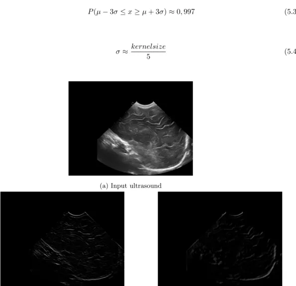
of the ROI needs to be done. A result from this process is given in Figure 3.

IV. PIXEL CLASSIFIER FOR SULCUS DETECTION

There are multiple different models created in order to get the best result. The models that are tested have different machine learning algorithms or the same algorithm but with different parameters. The first part of this chapter discusses the features trained on by the models. In the following part the results of the multiple created models are compared.

A. Model features – filter bank

The features consist of the results from multiple filters applied on the input image. This process is also known as applying a filter bank. There are two main types of filters used in this study. The first one is edge detection. This part exists of the difference of Gaussian and the Laplacian of the Gaussian distribution. Both are described in [9]. One handy characteristic from these filter is that they are orientated. This means that different results are achieved if the filter is applied to another direction in the image. Both filters are also dependent from the size of the gaussian kernel that is used and its standard deviation. These properties are very useful for machine learning algorithms because every combination of direction, size and standard deviation is another feature. In this way the result of the algorithm is not only dependable of a small number of features but a combination of all of them. It is also an interesting characteristic for detecting sulci. This mainly because sulci appear in multiple orientations and sizes in a certain ultrasound. For this reason this study applies the filters to a range starting from 0° to 150° with a step size of 30°. The size of the kernel varies from 3 by 3 to 41 by 41 and the standard deviation adjusts proportional with the kernel size based on the rule of thumb described in [10].

The second main type is ridge detection. Ridge detection is a technique that returns structures that follow a line pattern but are thicker than a simple line. It also filters out patterns like blobs and surfaces that are to wide too be a line. This is mainly done because the form of the sulci are more like ridges and not small edges. Edge detection showes the borders where the image intensities change abruptly, while ridge detection gives the whole ridge structure. Four filters are used for ridge detection. These are Sato’s three-dimensional filter for detecting curvilinear structures [11], Frangi’s multiscale vessel enhancement filter [12], Meijering’s filter for neurite tracing [13] and a Hybrid Hessian Filter [14]. They are all based on the direction of the second derivative of the image intensities. This can be achieved by looking at the eigenvalues of the Hessian

matrix of the image. The Hessian matrix for a 3D image is represented by Formula 1, 6 where Ixy(x, y, z) stands for

𝜕² 𝜕𝑥𝜕𝑦

I(x, y, z). Results from all these filters is given in Figure 4.

𝛻2_{𝐼(𝑥, 𝑦, 𝑧) = [} 𝐼𝑥𝑥(𝑥, 𝑦, 𝑧) 𝐼𝑥𝑦(𝑥, 𝑦, 𝑧) 𝐼𝑥𝑧(𝑥, 𝑦, 𝑧) 𝐼𝑦𝑥(𝑥, 𝑦, 𝑧) 𝐼𝑦𝑦(𝑥, 𝑦, 𝑧) 𝐼𝑦𝑧(𝑥, 𝑦, 𝑧) 𝐼𝑧𝑥(𝑥, 𝑦, 𝑧) 𝐼𝑧𝑦(𝑥, 𝑦, 𝑧) 𝐼𝑧𝑧(𝑥, 𝑦, 𝑧) ] (1)

B. Results pixel classifier

There are multiple machine learning models created for classifying the pixels into the sulcus class or background class. As a rooky in machine learning the first thing that has been done in this study is comparing different machine learning algorithms. The algorithms that are tried are random forest,

Figure 3: Result finding region of interest in ultrasound.

(a) Input ROI ultrasound

(b) Result DoG filter with kernel

size=7, σ=1.4, orientation=60° (c) Result DoG filter with kernel size=7, σ=1.4, orientation=60°

(d) Result Sato filter (e) Result Frangi filter

(f) Result Meijering filter (g) Result hybrid Hessian filter Figure 4: Results filterbank filters

stochastic gradient descent, quadratic discriminant analysis and support vector machine. To compare these models a 5-fold cross validation is done on the training dataset of 50 images discussed in Chapter III. An overview of the most important results is given in Table 1.

These results are only based on the DoG and LoG features, not the ridge features or a combination of them. Only the support vector machine model is not discussed in a table because based on a simpler test it took over 2 hours to do the fitting and around 21 minutes to test the scoring. This algorithm is thus dropped because of inefficiency. Table 1 shows that the random forest gives the overall best result because of a F1

score of 91,60 %. The stochastic gradient descent also works descent but doesn’t come close to the random forest with 82,68 %. With 68,88 % the quadratic discriminant analysis works is the worst of the three models. This all leads to the decision to continue this study only with the random forest model.

To give a view on how important the two types of features are, three different random forest models are built. The first two only have one of the type of the features and the third one combines both of them. The results of a 5-fold cross validation are shown in Table 2. From this table, it is clear that a random forest model with a combination of the features gives the best overall results with a F1 score of 95,25 %. The weight of both

features are comparable with a score of 91,60 % for the edge detection features and a 92,99 % for the ridge detection features. A visual result of the random forest model with the combination of features is given in Figure 5. From this figure can be concluded that the model does a good job in finding the sulci in the ultrasound, but there are still many false positives. For this

reason, some tricks are added to the get a better visual result. These are discussed in the next chapter.

To validate these results from the 5-fold cross validation based on the training data, the same test is done on a testing dataset of 25 ultrasounds that also have been hand labeled. This test leaded to a F1 score of 96,09 % that shows that the random forest

model with the combination of the edge detection and the ridge detection features has overall very good results.

(a) Input ROI ultrasound

(b) Labeled sulci by hand (c) Result classifier Figure 5: Result pixel classifier for detecting sulci

V. SULCUS ANALYSIS

After the model detects if pixels they are part of a sulcus or not, analysis of these sulci is needed. In this way doctors can use this study to evaluate the ultrasound of the brain of a preterm baby much quicker. It is also very hard to compare ultrasounds of the same infant on different timestamps which is needed to see the evolution of the brain during a certain treatment. This study could also help to overcome this problem.

To analyse the sulci, a skeletonized version is needed to calculate multiple parameters. How a skeleton is formed from the result of the sulci detector is discussed in the first part of this chapter.

There are two main metrics developed to help doctors analysing the ultrasounds. The first one determines the tortuosity of the whole sulcus. The second parameter calculates the length of the root branch of the sulcus. This is the original branch without bifurcations. As an extra feature to help analysing the ultrasounds, a different view at this study is taken. Except thinking as a doctor, this parameter is developed by looking at the image as an image processing engineer. The metric contains analysing the depth of the sulcus by looking at the pixel intensities of the intersection. All three of these metrics are explained in the there own section of this chapter.

A. Skeletonization of the sulci labels

As stated above, skeletonization or thinning of the detected sulci is needed to calculate all sorts of metrics. The implementation used in this study is from the scikit-image library. This one is based on the thinning algorithm of Zhang. The goal of this techniques is to thin the pattern to a uniform thickness of one pixel while distorting the endpoints and the connectivity of pixels as little as possible. [15]

Before the skeleton can be formed, a binary image is needed of only the sulcus where the skeleton needs to be formed from. A binary image is a digital image where the pixels have a value 0 for black or the value 1 for white. To only get the sulcus involved, labeling of the sulci is needed based on the result of the sulci pixel classifier. This can be achieved by using the scikit-image library again. The labeling method gives each pixel of a connected region a unique region value. A connected region is seen as neighbouring pixels have the same pixel value. After the labeling process, a binary image easily be created by copying only the pixels with the same value to a new image. After checking the output of the skeletonized versions, a lot of small branches and loops are found by the skeleton algorithm discussed above. This is because some pixels in the middle of the sulcus are classified as background pixels and the edges of the regions aren’t perfectly smooth. To solve this, a Gaussian blur with a kernel of 3 by 3 is applied to the output of the pixel classifier. The Gaussian blur filter is explained in [16]. The result of this is shown in Figure 6.

As mentioned in Chapter IV, where the labels are shown from the output of the pixel classifier, there are still many small pixel groups that actually are misclassified as sulci. To solve this, a

threshold is built that deletes contours with less then a certain amount of pixels. There is also an upper threshold built in this study. This should help if the boundary of the ROI, see Section III, is classified as a sulcus. A result from this thresholding is given in Figure 7 with a lower threshold value of 200 pixels. The upper threshold is not used for this image. This visualised result is the end result for detecting sulci in an ultrasound.

B. Tortuosity

Tortuosity is the first sulcus analysing parameter that is implemented. The tortuosity level tells how much a line is curved. This can be an interesting parameter to analyse sulci because a sulcus mostly starts as a simple line and develops in

Figure 6: Result skeletonization with and without Gaussian blur (a) Result skeletonisation without

Gaussian blur

(b) Result skeletonisation with Gaussian blur

(a) Labels before thresholding (b) Labels before thresholding

(c) Result skeletonization after thresholding. This is the end result for sulci detection in ultrasounds

Figure 7: Comparison labels after thresholding the area of the sulci with lower threshold = 200. This is an example end result for detecting sulci in an ultrasound.

all branches over the sum of the Euclidean distances between all the connected endpoints or intersections. The reason of this is that if the tortuosity of a bifurcated skeleton was defined as the mathematical mean of all the tortuosity levels of a branch, then it wouldn't give a correct result. The reason for this is that shorter branches are more tented to be straight and would way to much on the overall tortuosity level of the whole sulcus. To clarify more, Formula 2 is added.

𝑇𝑜𝑟𝑡𝑢𝑜𝑠𝑖𝑡𝑦 =

∑ 𝐵𝑟𝑎𝑛𝑐ℎ 𝑝𝑎𝑡ℎ 𝑙𝑒𝑛𝑔𝑡ℎ𝑠

∑ Euclidean distance between connected enpoints or intersections (2)

In order to find the endpoints, the intersections, and also calculate the lengths of the paths, a skeleton analysing library called Skan is used. The main advantage of this library is that it uses the Numba just-in-time (JIT) compiler to boost performance. It turns a skeleton image into a graph where all the pixels become nodes of the tree. Connected pixels become neighbouring nodes. It then simplifies the tree so only the intersections and endpoints remain nodes in the three. It becomes a weighted graph by coupling the distances between the intersections and endpoints to the remaining edges. The Skan library gives then the graph back in a scipy.sparce.csr matrix format. This is useful to do all sorts of tree algorithms on it. Skan makes it easy to just ask for the branch lengths and its Euclidean distances between the right endpoints or intersection. Calculation of the tortuosity with Skan is thus also very easy and performance wise at its best. [17]

C. Root branch length

Another common used parameter to analyse sulci is the length of the original or root branch of the sulcus. To find this root branch is not always easy because of the non regularity in the sulci and its locations in the ultrasounds. This study mainly focusses on preterm infants as stated many times above. The sulci of these babies are still in early stages of development. That is why this study pairs the next definition to find the main branch of a sulcus. The root branch is defined as the longest shortest path between two endpoints. This solution gives good results with simple sulci but have problems with complex ones. A result from this root branch searching is visualised in Figure 8. Here is the root branch visualised in yellow pixels.

main advantage of using the Skan library to get the length of a branch is that it uses the rule of pythagoras to calculate the length of neigbours that are aligned diagonally. In this way the length is more realistic. To get the length in cm, a realistic units of length, multiplying the length based on pixels with the scale of the ultrasound is done. This scale can be achieved from reading the DICOM attributes discussed in section III. [19]

D. Depth analysing by looking at pixel intensities of an intersection of a sulcus

After brainstorming for more analysing metrics, the idea rose up to look at this study more from an image processing engineer standpoint. This led to developing a metric that checks the intensity values of an intersection of a sulcus. In this way, this metric could give a visualisation of the depth of the sulcus by showing a graph of the intensities. After discussing this with a trained doctor in analysing brains of preterm babies (dr. P. Govaert of ZNA middelheim), this metric isn’t useful for further purposes. This is mainly because an ultrasound is just a visualisation of a part of the inner body and gives no real measurements of how deep something is located.

VI. USABLE TOOL

This study is for obvious reason useless if there wasn't a way that doctors can use these analysing techniques in a handy and easy accessible tool. This is done in two ways. The more accessible and easy manner is that doctors can use this through a webtool that is all the time available with an internet connection. A problem with a webtool is that adjusting options are limited. For this reason there is also a graphical user interface or GUI built. This GUI is built during the developing times and was mainly meant for just testing purposes, not really for deployment. The GUI isn't dropped because it still had some advantages such as some adjusting abilities. These means that a user can delete detected sulci and adjust some of them by drawing on the predicted labels image. The user can then rerun the program and it will calculate the new sulci based on the adjusted labels.

VII. FUTURE WORK

One of the goals of this thesis was to do a fully automatic analysis of an ultrasound with clear sulci visible of a preterm baby. For this to happen, the analysis needed to output a predicted gestational age (GA) based on the metrics defined in Chapter 6. This isn’t the case up to this moment. The study should need some extra work. The main thing that is lacking, is a classifier that can detect and name the most important sulci like the Central sulcus and the Lateral sulcus. This is needed because a brain contains many minor different sulci that are very variable in location, size and tortuosity. In this way it is very hard to determine the GA of a random ultrasound without knowing where the most important ones are located. These have

Figure 8: Example of finding the root branch by searching for the longest shortest path between

the advantage that they are already quite large at the stage 28 week GA and start to develop into a more and more curvature in them. A second difficulty is that an ultrasound doesn’t give a whole view of a certain brain but just a small section. This all leads to a difficult task for the future, but is definitely not impossible.

VIII. CONCLUSION

In this master’s dissertation a tool is proposed to analyse the sulci of a preterm baby in an ultrasound image. This is done by building a pixel classifier that detects if a pixel belongs to a sulcus or not. This machine learning model is based on a random forest of a dataset of around 50 ultrasound of clear patterns of sulci. The model uses edge and ridge detection techniques as features. The classifier works quite well with a F1 score of 95,25 % on the training data and 96,09 % on the testing data. After the pixels are classified in to sulcus pixels or background ones, some analysing metrics are proposed. These are based on the skeletonised version of the labels of sulci. The metrics developed are a tortuosity level of the whole sulcus, the length of the root branch and a depth analysing graph that looks at the intensity values of an intersection of a sulcus. This study would be useless if there wasn’t a way for doctors to use it. For this reason a GUI and a web application is built. The GUI is developed more for testing purposes and the website for deployment. The GUI isn’t dropped because it has some advantages such as adjusting the detected labels.

REFERENCES

[1] K. Im and P. E. Grant, “Sulcal pits and patterns in developing human brains,” jan 2019.

[2] “LGI - Free Surfer Wiki.” https://surfer.nmr.mgh.harvard.edu/fswiki/LGI. Accessed: 2020- 08-07. [3] J. Zhang, “Secrets of the Brain: An Introduction to the Brain Anatomical

Structure and Biological Function,”

[4] P. V. Bayly, K. E. Garcia, and C. D. Kroenke, “Mechanics of cortical folding: stress, growth and stability,”

[5] V. Rajagopalan, J. Scott, P. A. Habas, K. Kim, J. Corbett-Detig, F. Rousseau, A. J. Barkovich, O. A. Glenn, and C. Studholme, “Development/Plasticity/Repair Local Tissue Growth Patterns Underlying Normal Fetal Human Brain Gyrification Quantified In Utero,” 2011

[6] The DICOM Standards Committee, “DICOM PS3.1 2020c - Introduction and Overview,” tech. rep., 2020

[7] innolitics, “US Image CIOD – DICOM Standard Browser.” https://dicom.innolitics.com/ciods/us-image. Accessed: 2020-07-17 [8] S. Suzuki and K. A. Be, “Topological structural analysis of digitized

binary images by border following,” Computer Vision, Graphics and Image Processing, vol. 30, no. 1, pp. 32–46, 1985.

[9] L. Assirati, N. R. Silva, L. Berton, A. A. Lopes, and O. M. Bruno, “Performing edge detection by Difference of Gaussians using q-Gaussian kernels Related content A shader for simultaneous ambient occlusion and edge detection for reverse engineering-A Novel Method for Edge Detection in Images Based on Particle Swarm Optimization-The edge detection enhancement on satellite image using bilateral filter-Recent citations Performing edge detection by Difference of Gaussians using q-Gaussian kernels,” Journal of Physics: Conference Series OPEN ACCESS

[10] A. Ramirez and C. Cox, “Improving on the Range Rule of Thumb,” Tech. Rep. 2, 2012.

[11] Y. Sato, S. Nakajima, N. Shiraga, H. Atsumi, S. Yoshida, T. Koller, G. Gerig, and R. Kikinis, “Three-dimensional multi-scale line filter for segmentation and visualization of curvilinear structures in medical images,” Medical Image Analysis, vol. 2, pp. 143–168, jun 1998. [12] A. F. Frangi, W. J. Niessen, K. L. Vincken, and M. A. Viergever,

“Multiscale vessel enhancement filtering,” in Lecture Notes in Computer

Science (including subseries Lecture Notes in Artificial Intelligence and Lecture Notes in Bioinformatics), vol. 1496, pp. 130–137, Springer Verlag, oct 1998.

[13] E. Meijering, M. Jacob, J.-C. Sarria, P. Steiner, H. Hirling, and M. Unser, “Design and validation of a tool for neurite tracing and analysis in fluorescence microscopy images,” Cytometry, vol. 58A, pp. 167–176, apr 2004

[14] C. C. Ng, M. H. Yap, N. Costen, and B. Li, “Automatic wrinkle detection using hybrid Hessian filter,” in Lecture Notes in Computer Science (including subseries Lecture Notes in Artificial Intelligence and Lecture Notes in Bioinformatics), vol. 9005, pp. 609–622, Springer Verlag, 2015. [15] T. Y. Zhang and C. Y. Suen, “A Fast Parallel Algorithm for Thinning

Digital Patterns,” tech. rep., 1984

[16] E. Gedraite and M. Hadad, “Investigation on the effect of a gaussian blur in image filtering and segmentation,” pp. 393–396, 01 2011.

[17] J. Nunez-Iglesias, A. J. Blanch, O. Looker, M. W. Dixon, and L. Tilley, “A new Python library to analyse skeleton images confirms malaria parasite remodelling of the red blood cell membrane skeleton,” [18] M. A. Javaid, “Understanding Dijkstra Algorithm,” SSRN Electronic

Journal, oct 2013.

[19] “NetworkX — NetworkX documentation.” https://networkx.github.io/. Accessed: 2020-07- 19.

Contents

Preamble concerning COVID-19 iii

Preface v

Admission to loan vii

Abstract ix

Extended abstract xi

1 Introduction 1

2 Literature Study 3

2.1 The human brain . . . 3

2.1.1 Basic brain anatomy . . . 3

2.1.2 Cerebral cortex . . . 4

2.1.3 Process of gyrification . . . 5

2.2 Machine learning models . . . 6

2.2.1 Random forest . . . 6

2.2.2 Stochastic gradient descent . . . 7

2.2.3 K-fold cross-validation . . . 7

3 Related work 11 4 Dataset 13 4.1 Training and testing dataset creation . . . 13

4.2 The DICOM standard . . . 14

4.3 Region of interest (ROI) . . . 15

4.3.1 Suzuki’s algorithm to obtain the topological structure of an image . . . 16

5 Pixel classifier for sulcus detection 21 5.1 Model features - filterbank . . . 21

5.1.1 Edge detection . . . 21

5.1.2 Ridge detection . . . 24

6 Sulcus analysis 37 6.1 Skeletonization of the sulci labels . . . 37 6.1.1 Cleaning of skeletonization - results . . . 39 6.2 Tortuosity . . . 42 6.3 Root branch length . . . 44 6.3.1 Dijkstra’s shortest path algorithm . . . 44 6.4 Depth analysis by looking at pixel intensities of an intersection of a sulcus . . . 45

7 Usable tool 47

7.1 Web application . . . 47 7.2 Graphical user interface (GUI) . . . 51

8 Future work 55

List of Figures

2.1 The four main parts of a basic anatomic view of the human brain, including the brainstem, the cerebellum, the diencephalon and the cerebrum [1] . . . 4 2.2 A lateral view of the cerebral cortex with the division of the four lobes [2] . . . 5 2.3 The three stages of cortical folding or gyrification [3] . . . 6 2.4 visualisation of a random forest [6] . . . 7 2.5 visualisation of a 3-fold cross validation [8] . . . 8 3.1 visualisation GI. GI is equal to the ratio of the surface of the red part to the one of

the red part like defined in Formula 3.1 [10] . . . 12 4.1 Example of an training data image and its labeled version . . . 14 4.2 General Communication model of the DICOM protocol for exchanging medical

im-ages [11] . . . 15 4.3 Result finding ROI in ultrasound image . . . 16 4.4 visualisation of the definitions of an outer border and a hole border. The outer

border is coloured red and the hole border green. . . 17 4.5 visualisation of a raster scan [15] . . . 18 4.6 Example of the Suzuki’s topological structure analysis algorithm [14] . . . 19 5.1 Difference of Gaussian (DoG) with σ = 2, 5 vs Laplacian of Gaussian with σ1= 2, 5

and σ2= 2, 15 [16] . . . 22

5.2 Results DoG and LoG filters on example ultrasound . . . 23 5.3 The two weight function for deviations from there conditions [18] . . . 26 5.4 Example ultrasound input with noisy blob-like patterns in the lower part of the image 27 5.5 Result Sato filter on an example ultrasound . . . 27 5.6 Result Frangi filter on an example ultrasound . . . 29 5.7 Result Meijering filter on an example ultrasound . . . 30 5.8 Result Hybrid Hessian filter on an example ultrasound . . . 31 5.9 Result pixel classifier for detecting sulci . . . 34 6.1 Labeling of the pixels in the 3 by 3 window [23] . . . 38 6.2 Example of the thinning algorithm of Zhang [23] . . . 39 6.3 Comparison skeletonization of labels with and without Gaussian blur . . . 40

6.4 Comparison labels after thresholding the area of the sulci with lower threshold = 200. This is an example of an end result for detecting sulci in an ultrasound . . . . 41 6.5 Three different definition of the tortuosity level of a line [25] . . . 43 6.6 The tortuosity definition used in this study to get an overall correct result of the

whole sulcus. The tortuosity equals the ratio of the sum of all orange path lengths divided by the sum of all the blue paths (Formula 6.5) . . . 43 6.7 Example of finding the root branch by searching for the longest shortest path

be-tween two endpoints . . . 44 6.8 Example depth analysis of sulcus by mapping intensity values . . . 46 7.1 Upload page web application . . . 48 7.2 Uploaded ultrasound with DICOM attributes . . . 48 7.3 Result sulci detection on web application . . . 49 7.4 Labels section of results web application . . . 50 7.5 Sulci analysing section of results web application . . . 51 7.6 Graphical user interface for testing purposes . . . 52 7.7 Result from the ”DELETE SULCUS” process . . . 53 7.8 Result from the ”ADJUST LABELS” process . . . 54

List of Tables

2.1 Definition of TP, TN, FP and FN . . . 8 4.1 Decision table for the parent border of the newly found border B [14] . . . 18 5.1 Detected structure type based on the signs and values of the eigenvalues of the 2D

and 3D Hessian matrix (H = high value, L = low value, N = noisy, + = positive sign and - = negative sign) [18] . . . 29 5.2 Result 5-fold cross validation based on a random forest model of only the edge features 31 5.3 Result 5-fold cross validation based on a stochastic gradient descent model of only

the edge features . . . 32 5.4 Result 5-fold cross validation based on a quadratic discriminant analysis model of

only the edge features . . . 32 5.5 Result 5-fold cross validation based on a random forest model of only the ridge features 33 5.6 Result 5-fold cross validation based on a random forest model of a combination of

the edge detection and the ridge detection . . . 33 5.7 Result 5-fold cross validation based on a random forest model of a combination of

Chapter 1

Introduction

Medical imaging is a very time consuming task for doctors and in the latest trends, the demand for them still growing. This could lead to a shortage of trained doctors to take and analayse them. That’s why it is important that there are more studies dedicated to automatically analysing med-ical images.

This study is dedicated to automatically analyse cerebral sulci of preterm babies in ultrasound images. The sulci are the grooves in a human brain and the development of them are crucial for our intellectual level. These start to form during pregnancy and develop through our whole life. This process is called gyrification. Sulci are always paired with gyri that are the ridges of a human brain. It is important to analyse these with preterm babies because the main part of the gyrification process takes place during the third trimester of pregnancy. This is the stage where preterm babies are born. If there are at that stage some serious deviations in the gyrification process detected, doctors could still try to help the infant.

It also important to notice that the images used in this study to analyse the sulci of a preterm baby are ultrasounds. An ultrasound has some disadvantages over other medical imaging techniques, but for this study they also have some handy advantages. The main disadvantage is that a basic understanding is needed to understand the image. For example, The orientation and location of the image is needed because it doesn’t represent the whole brain in one image. It also has some problems with noise artifacts. A major advantage of using ultrasounds in this study is that the doctor who is taking them, can easily adapt to the movement of a preterm baby. This is important as some imaging techniques demand that the patient lays perfectly still for a certain amount of time and this is very hard for a baby that age.

The first chapter of this study is a literature study that contains a basic introduction to the anatomy of a human brain and the process of gyrification. The chapter further includes some machine learning models that are used in this research and a technique to compare such models. A related study based on magnetic resonance images is discussed in the next chapter. Chapter 4 contains information of the dataset that is used for creating a pixel classifier for detecting sulci . The next chapter discusses the pixel classifier. Section 6 describes the metrics that are developed

for analysing the detected sulci. Since this study is useless if there wasn’t a way for doctors to use it, it’s applicability in medicine is explained in Chapter 7. The following section proposes possibilities of future work that could be done on this study. Finally, a conclusion of this thesis is given

Chapter 2

Literature Study

In this chapter a short literature study is given so that a basic understanding for the start of this study is clear. The first part contains information on the anatomy of the human brain and how it develops into the stage of a full grown baby. This is important because this study focusses on preterm babies. In the second part a short introduction to the main machine learning models is given which are used in this study to detect sulci in an ultrasound. These models are random forest and stochastic gradient descent.

2.1

The human brain

Before any work can be done on automatic analysis of the cerebral sulci, a basic understanding of the anatomy of the human brain is needed. This is given for a normal full grown cerebrum in the first part of this chapter. Because of the importance of the cerebral cortex compared to the other parts of the brain anatomy a further explanation is noted in a separate section. This study mainly focuses on analysis of the sulci of preterm babies. These are newborns that are actually born too early. In numbers, this is before 40 weeks gestational age (GA). For this reason, the third part of this chapter contains how the outer region of the brain develops into the stage of 40 weeks GA.

2.1.1

Basic brain anatomy

The human brain exists of hundreds to thousands parts that all have their own function. A basic anatomic view divides it in four main parts. This is visualised in Figure 2.1. The four parts are named the brainstem, the cerebellum, the diencephalon and the cerebrum. All of these will be explained briefly so a basic understanding of the whole brain is clear.

Figure 2.1: The four main parts of a basic anatomic view of the human brain, including the brainstem, the cerebellum, the diencephalon and the cerebrum [1]

The first region is called the brainstem. This is the part that connects the basis of the brain to the spinal cord by linking multiple parts of the nerve system.

The cerebellum is the next main division of the basic anatomy explanation. It is located at the lower back of the brain and is important for controlling motor functions such as balance. The cerebellum is also very active while processing language, paying attention to something and regulating some emotions such as pleasure or fear.

The third major part is the diencephalon and is situated at the center of the cerebral above the brainstem. In some other anatomic divisions of the brain only exists of three main parts. The diencephalon is then included in the brainstem. It is responsible for regulating respiratory and cardiac functions as well as handling sleeping and eating functions. A large part of the diencephalon, called the thalamus, receives a great part of the information from the cerebral cortex, processes it and sends information back to other regions of the brain.

The last segment is called the cerebrum and is the outer region of a brain. This one mainly exists of the cerebral cortex. The cerebrum is the region where all the human thoughts, judgements and memory functions are located. It also plays a major role in voluntary motor activities. The cerebrum is the most import part of the brain for this study because it is the only visible part in an ultrasound image and gives a great representation of how mature the brain is. This is because the human brain goes through the process of gyrification during pregnancy and early stages of childhood. Gyrification will be explained in Section 2.1.3. Because of the importance of the cerebral cortex for this study, a deeper anatomic explanation will be given in the next part of this chapter (Section 2.1.2). [2]

2.1.2

Cerebral cortex

The cerebral cortex is the outer layer of brain tissue. It exists of two almost symmetric hemispheres. These are separated by the longitudinal fissure. The process of gyrification causes the cortex to be folded in ridges, called gyri and grooves, called sulci. These are formed so that the outer surface area increases. In this way more cognitive power is available to a human being. The locations of

sulcus. The parietal lobe mainly focuses on sensory information such as navigation and touch. The occipital lobe is located at the lower back of the human brain and processes mainly vision. The temporal lobe, at last, lies under the lateral sulcus that runs at the lower ends of the frontal and parietal lobes. The temporal lobe is active while processing visual memory, language and emotions. [2]

Figure 2.2: A lateral view of the cerebral cortex with the division of the four lobes [2]

2.1.3

Process of gyrification

As stated above, gyrification is the process where the brain folds the cerebral cortex and develops gyri and sulci. Gyri are the ridges that are formed and the sulci are the grooves. There are three stages of cortical folding. The primary gyri and sulci are formed during the second trimester of pregnancy. This starts around 13 weeks GA and ends at the 27th week. The primary sulci consists mainly of the central and the lateral sulcus. The secondary and tertiary folding are developed in the third trimester. In the secondary stage the central and lateral sulcus are developed even further and some other ones are formed. Later stages of the secondary folding and the whole tertiary one are very hard to describe and quantify. This is because positions of sulci vary very much from some standard patterns. This study focuses mainly on preterm babies. These are infants that are still in the secondary stage of the folding process. In Figure 2.3 is a timeline given of the gyrification stages with a 3D model of a human brain in those three stages. [3, 4]

Figure 2.3: The three stages of cortical folding or gyrification [3]

2.2

Machine learning models

In this chapter a basic explanation of the machine learning models that are used in this study will be given. The models that will be explained are a random forest and a stochastic gradient descent. There will also be a part written about the k-fold cross validation technique because it is used to compare the different models created with each other.

2.2.1

Random forest

The random forest machine learning algorithm is based on decision trees. A decision tree is built by splitting the pre-classified dataset multiple times based on the feature that at that point divides the set the best. In this way an end nodes represent a certain class. This leads to a model using discriminative classification. They have the advantage that they are effective and have understand-able rules for humans on classification. The problem with them is that when the dataset grows, more splitting and reordering off the dataset is needed and this is very costly based on efficiency and memory. This is where the random forest model comes in handy.

The random forest model is defined as a group of un-pruned decision trees made from random parts of the training data. In this way the eventual classification is decided based on the majority vote. They are considered as a general purpose computer vision machine learning model. A random forest has the following advantages over a single decision tree. A visualisation of random forest existing of three trees is given in Figure 2.4. [5]

• No over fitting the training set.

• Less sensitive to outliers in the training set. • Can handle larger datasets.

Figure 2.4: visualisation of a random forest [6]

2.2.2

Stochastic gradient descent

Stochastic gradient descent is based on the mathematical technique to solve optimization problems called gradient descent. Gradient descent starts with an initial vector w0 that is randomly chosen

and iteratively perform Formula 2.1 to get the optimal vector for the function f (). The function f () represents a loss function. This means that it defines the deviation from all the data points. These vectors used in gradient descent is a combination of all the features. An important property of Gradient descent is that it takes big values for α or big step sizes if the value is far from the optimal value and smaller ones when it’s closer. This causes a major boost in efficiency. This step size is always multiplied with a predefined learning rate. This learning rate is important for how fast it gets to a good result but it is possible that the achieved result is not the most optimal one when the learning rate is too high. The algorithm stops when the step size multiplied with the learning rate is smaller than a predefined parameter or when a maximum amount of iterations is achieved.

wk+1= wk− αkOf (wk) (2.1)

There are two major problems with gradient descent. The first one is that sometimes not all the gradients can be exactly calculated. The second problem includes that gradient descent needs to calculate a derivative for every feature existing of as many terms as data points. This takes a lot of computational power. This means that gradient descent is very slow for big data. This is where stochastic gradient descent comes in handy. Stochastic gradient descent takes a random selected vector γk based on only one data sample and calculates only the corresponding derivatives and

performs Formula 2.2 iteratively. In this way stochastic gradient descent becomes very efficient with big data and it gets similar results as gradient descent. [7]

wk+1= wk− αkγk (2.2)

2.2.3

K-fold cross-validation

A cross-validation is a statistical technique for evaluating machine learning models. This is done by dividing the dataset in two parts. The first part is for training the model and the second one

for validating or testing. Often this method is repeated for some iterations so that each data point has a chance of being validated against the other data points. This is done by redistributing the dataset. There are multiple popular cross-validating techniques. The one used in this study is the k-fold cross-validation method. [8]

The k-fold validation method partitions the dataset into k equally sized parts. It does cross-validation for k iterations and uses k-1 segments for training the model and one for validating. Each iteration another set is used for the validation. In this way an overall view on the performance of the created model is achieved. In Figure 2.5 a visualisation of a 3-fold cross validation is given.

Figure 2.5: visualisation of a 3-fold cross validation [8]

To compare models against each other, multiple metrics are needed. There are many different types but the ones most used are the accuracy, the precision and the recall of the dataset. An other very popular metric is the F1-score. This one combines the recall and precision and gives

more an overall performance view of the dataset. How these are defined is given in the Formulas 2.3 until 2.6. These use the abbreviations defined in Table 2.1.

Table 2.1: Definition of TP, TN, FP and FN Prediction

Positive Negative

Ground truth

Positive True positive (TP) False negative (FN) Negative False positive (FP) True negative (TN)

Accuracy = # Correctly predicted # T otal predictions =

T P + T N

T P + T N + F P + F N (2.3)

P recision =# Correctly predicted positive # T otal predicted positive =

T P

T P + F P (2.4)

Recall = # Correctly predicted positive # T otal correct predictions =

T P

Chapter 3

Related work

This isn’t the first study that dedicates its time to try to automatically analyse cerebral sulci. One of the most important ones on this subject is a study done by the medical school of Harvard University. This research led to a matric that maps very well to the gestational age (GA) of a brain. This metric is called the Gyrification Index (GI) and it quantifies amount of cortex within the folds of the sulci compared to the amount that is visible on the outer part of the brain. In formula form is this Formula 3.1 and a visualisation of this is given in Figure 3.1. In this image the GI is equal to the ratio of the surface of the red part to the one of the yellow part. It also looks at local patterns of GI around sulcal pits. These are the deepest local regions of sulci because of the early forming of the first cortical folds. [9, 10]

This measurement based on GI could be very handy because the pattern of primary sulci only varies a little during the end of a normal pregnancy or with preterm infants. If there are some serious variations at that point of a human life, this may reflect into problems with cognitive func-tion, personality problems or psychiatric disorders.

The main problem with this study is that it’s based on magnetic resonance images (MRI’s). This is an medical imaging technique where it is needed to let the patient lay perfectly still for a certain amount of time. This is definitely a problem with preterm babies. For this reason it would be very interesting to have some of the same results based on ultrasound images, where a trained doctor can easily adopt to the movements of a baby.

GI = Surf ace of cortex within the f olds of the sulci

Figure 3.1: visualisation GI. GI is equal to the ratio of the surface of the red part to the one of the red part like defined in Formula 3.1 [10]

Chapter 4

Dataset

This chapter discusses how the dataset is formed and what it contains. The first part explains how the training dataset for the machine learning is achieved. This is a carefully selected part from the whole dataset that is available for this study. The dataset exists of DICOM files. This file extension is not very well known outside of the medical sector. For this reason, the second part of this chapter discusses the DICOM file extension and what the DICOM standard is. The last part of this section explains how the input ultrasound is adjusted to only get the actual ultrasound part. This process is needed so that other parts of the image don’t effect the pixel classification results. This part is the region of interest or ROI for the machine learning model.

4.1

Training and testing dataset creation

The dataset that is available for this study exists of approximately 3000 DICOM files of ultrasounds of the cerebral cortex of over 30 preterm babies in total. From this set a training data needs to be created for the pixel classifier. The classifier needed to detect if a pixel represents a part of a sulcus or not. A lot of images needed to be discarded from the dataset to get a good training data. This was mainly because only the sagittal or side view of the brain show clear patterns of sulci. Thus, all the transverse views (top view) needed to be dropped. A second reason why an ultrasound could be dropped is because of a clear attendance of noise in the images. The second part in the process of creating the training data was labeling the sulci. All the pixels that are part of a sulcus are drawn in white and the others in black. The labeling is not done by a trained professional but by the researcher self (R. De Smet), so here errors can occur. Because this process was very time consuming, only 75 images of the entire dataset are processed and filtered. This all lead to a training data of 50 and a testing set of 25 clear ultrasounds of sagittal views of the brain with labeled sulcus data. Of course this training data could be expanded in later developments of this study but it already resulted in quite good results for detecting sulci. An example of a training data image and its labeled version is given in Figure 4.1.

(a) The training data image (b) Labeled version

Figure 4.1: Example of an training data image and its labeled version

4.2

The DICOM standard

DICOM stands for Digital Imaging and Communication in Medicine and is a standard for the management and communication of medical images and related patient data. The DICOM organi-zation developed a file format for medical images and a protocol for exchanging these. The DICOM standard is recognized by the International Organization for Standardization as ISO 12052. Nowa-days, almost every medical imaging machine is implemented to support it. The main advantage of DICOM is that it groups information into data sets. This means that medical images are directly linked with information of the patient in the DICOM file. For this reason useful images couldn’t get lost. [11]

The linking of the information to the medical image is done by including attributes to the DICOM file. There are over 2000 standard attributes. These can be achieved by calling their name or their corresponding hex code. The important ones for this study are listed below. [12]

• (0010, 0020) Patient ID: Unique identification number of the patient • (0010, 0010) Patient’s Name: Name of the patient

• (0010, 0030) Patient’s Birth Date: Birth date of the patient (JJJJMMDD) • (0008, 0080) Institution Name: Institution name of where the image was taken • (0018, 602c) Physical Delta X: Scale pixels to cm in horizontal direction • (0018, 602e) Physical Delta Y: Scale pixels to cm in vertical direction

The communication protocol will not be discussed because it is not used in this study. To give a brief view of what the protocol includes, Figure 4.2 is added.

Figure 4.2: General Communication model of the DICOM protocol for exchanging medical images [11]

4.3

Region of interest (ROI)

An ultrasound image exists of the actual ultrasound visualisation and a lot of parameters about the patient and the ultrasound settings. These extra text is not interesting for the machine learning model for classifying pixels into a sulcus class or background class. It could also influence the result of the model because the text in the image are also intensity changes and could be seen as edges or ridges. The classifying model is discussed in Chapter 5.

Finding the ROI is done by finding all the contours in the ultrasound image with the help of the OpenCV library. This library has a method built in, called cv2.findContours(). It returns all the available contours based on Suziki’s algorithm to find a topological structural analysis in digitalized binary images. This algorithm will be discussed in the next subsection (Section 4.3.1). The actual ultrasound visualisation in the image is then the contour with the largest area. All the pixels in that area are assigned with value 1 and all the others with value 0. In this way a binary image is created with only the ROI. To obtain the original image with only the ultrasound visualisation, a multiplication of the corresponding pixels of the original image and the binary image of the ROI needs to be done. A result from this process is given in Figure 4.3. [13, 14]

(a) Original ultrasound (b) Largest contour = ROI

(c) Multiplication of the original ultrasound with the ROI

Figure 4.3: Result finding ROI in ultrasound image

4.3.1

Suzuki’s algorithm to obtain the topological structure of an image

Suziki designed an algorithm to obtain the topological structure of a binary image. A binary image is an image where the values of the pixels are either 1 or 0. The algorithm finds all the contours in the image by following along with the borders of them and finds the topological structure of them. This means that it finds which contours lay in one another and vice versa. Suzuki defines a border as a sequence of pixels between connected components of 1-pixels and 0-pixels. This algorithm also makes a difference between two types of borders, hole borders and outer borders. An outer border is defined as the one of an 1-component that is directly surrounded by a 0-component. Hole borders are than the opposite. To make these definitions more clear, Figure 4.4 is added. In this figure pixels with the value 0 are coloured black. White pixels are pixels with the value 1. The red border in this figure represents an outer border and the green one a hole border. [14]

Figure 4.4: visualisation of the definitions of an outer border and a hole border. The outer border is coloured red and the hole border green.

Suzuki’s algorithm is explained in the following steps. In these fi,j stands for the assigned label

for pixel at location (i, j). The horizontal direction is represented by the letter j and the vertical one by i. It also uses two other variables α and β to later assign to the labels of the border pixels. Step 1: Start a raster scan like in Figure 4.5. Set variable α to 1 and the labels of all the border

pixels to 1.

Step 2: Select a pixel from the raster scan if it satisfies one of the following statements:

(a) If fi,j = 1 and fi,j−1 = 0 then is that pixel the starting point for an outer border.

Increment α by 1 and set pixel (i2, j2) ← (i, j − 1).

(b) Else if fi,j ≥ 1 and fi,j+1 = 0 then is that pixel the starting point for a hole border.

Increment α by 1 and set pixel (i2, j2) ← (i, j + 1).

(c) Otherwise, go to Step 5.

Step 3: Decide the parent of current border depending on the type of the border and the variable β by applying Table 4.1. This β variable is the label of the last found border on the same row of the current starting pixel.

Step 4: Start from the starting pixel (i, j) and follow the detected border by applying the next steps: (a) Select the next nonzero pixel in the direct neighbourhood of (i, j) by looking clockwise starting from the direction with (i2, j2) and denote it as (i1, j1). If no nonzero pixel is

found assign −α to the label of pixel (i, j) and go to Step 5. (b) Assign: (i2, j2) ← (i1, j1) and (i3, j3) ← (i, j).

(c) Select the next nonzero pixel in the neighbourhood of (i3, j3) by looking counterclockwise

starting from the direction with (i2, j2) and denote it as (i4, j4).

(d) Change the label of the pixel (i3, j3) or fi3,j3 as one of the following:

(i) If (i3, j3+ 1) is a 0-pixel then assign fi3,j3= −α

(ii) Else if (i3, j3+ 1) is a 1-pixel and fi3,j3 = 1 then assign fi3,j3 = +α

(e) If (i4, j4) = (i, j) and (i3, j3) = (i1, j1) (or with word if the starting point is achieved

again), then go to Step 5. Otherwise, assign: (i2, j2) ← (i3, j3) and (i3, j3) ← (i4, j4)

and go back to Step 4c.

Step 5: If fi,j 6= 1 then assign β = |fi,j| and resume the raster scan until the lower right corner is

achieved from the image.

Notice that this algorithm also assigns a label to the outer border of the image. This border gets the label 1 assigned to it. An example of this algorithm is given in Figure 4.6.

Figure 4.5: visualisation of a raster scan [15]

Table 4.1: Decision table for the parent border of the newly found border B [14] Type of border B’ with the label β

Outer border Hole border

Type of the current border B Outer border The parent border of B’ The border B’ Hole border The border B’ The parent border of B’

Chapter 5

Pixel classifier for sulcus detection

This chapter discusses how the machine learning model is created to detect if a pixel is part of sulcus or not. It is thus a pixel classifier with only two classes. This problem can be seen as a foreground and background detector. The first section of this chapter contains information about which features are used to detect the sulci in the ultrasound. This is done by applying multiple filters to ROI of the original image in a filterbank. The filterbank exists of two edge detection techniques and four ridge detection ones. The result of each filter is then used as a feature.

There are multiple different models created to try to get the best result. The models that are tested have different machine learning algorithms or the same algorithm but with different parameters. All of them are discussed and compared in the second section of this chapter. There are also the overall results of the classifier stated.

5.1

Model features - filterbank

In this section of the chapter the features used to detect sulci pixels in an ultrasound image are explained. The features exist of the results from multiple filters applied on the input image. This is also known as applying a filterbank. There are two main types of filters used in this study. The first one is edge detection. This part exists of the difference of Gaussian and the Laplacian of the Gaussian distribution. The second main type is ridge detection. This is mainly done because of the form of the sulci are more like ridges and not small edges. Edge detection gives the borders where the image intensities change abruptly, while ridge detection gives the whole ridge structure. Four filters are used for ridge detection. These are Sato’s three-dimensional filter for detecting curvilinear structures, Frangi’s multiscale vessel enhancement filter, Meijering’s filter for neurite tracing and a Hybrid Hessian Filter.

5.1.1

Edge detection

To perform edge detection on the ultrasound image, two techniques are used. These are Difference of Gaussian (DoG) and the Laplacian of Gaussian (LoG). Both of these are closely related, but they do have their advantages above each other. The two-dimensional gaussian distribution is noted in