Deep learning for high resolution 3D positioning of gamma interactions in monolithic PET detectors

(1)

gamma interactions in monolithic PET detectors

Deep learning for high resolution 3D positioning of

Academic year 2019-2020

Master of Science in Engineering Physics

Master's dissertation submitted in order to obtain the academic degree of

Counsellors: Mariele Stockhoff, Ir. Milan Decuyper

Supervisors: Prof. dr. Stefaan Vandenberghe, Prof. dr. Roel Van Holen

Student number: 01405296

Pieterjan De Boose

(2)

(3)

Permission of use on loan

The author gives permission to make this master dissertation available for consultation and copy parts of this master dissertation for personal use. In all cases of other use, the copy right term has to be expected, in particular with regard to the obligation to state explicitly the source when quoting results from this master dissertation.

August 2, 2020 Ghent

(4)

Acknowledgement

This thesis was not in any case possible without my promotors Prof. dr. Stefaan Vandenberghe and Prof. dr. Roel Van Holen of Ghent University and in particular the MEDISIP laboratory. Their phenomenal work continues to push boundaries and creates an environment of learning of which I feel grateful to have been a part of.

Furthermore, I direct my utmost gratitude to my counsellors ir. Milan Decuyper and Mariele Stockhoff for their insightful and compassionate guidance along the way uphill and wish them a bright future. I would also like to thank their colleagues Jurgen and Jens to help me to remotely access the lab computer which allowed me to finish my thesis in times of the COVID-19 pandemic.

A warm heart goes out to my family, my parents Lut Van De Velde and Johan de Boose for their continuous support and patience throughout enduring times, and the legendary Gemini, my sister Mira de Boose and oma Imelda. Lastly, I reflect on the unforgettable days and nights of joy, peace, drama, laughter and much more that I lived and survived with my dear friends Michiel De Kesel, C´eline Thijs and Tim Van Welden, and I cannot wait to see what the future holds for all of us.

Thank you all from the bottom of my heart. Pieterjan de Boose, August 8 (Ghent)

(5)

(6)

Deep learning for high resolution 3D positioning of

gamma interactions in monolithic PET detectors

Pieterjan de boose

Master of Science in Engineering Physics

Faculty of Engineering and Architecture (Ghent University)

Supervisors: Prof. dr. Stefaan Vandenberghe, Prof. dr. Roel Van Holen

Counsellors: ir. Milan Decuyper, Mariele Stockhoff

Abstract

Major limitations facing PET-scanners today include low sensitivity and spatial resolution, and high cost [62]. Monolithic scintillation detectors, as opposed to pixelated detectors, are one of the promising op-tions being investigated today. Besides the absence of dead space which degrades sensitivity, the spatial resolution of a continuous configuration is not limited by pixel size. Positioning a γ-interaction within the detector block can be performed by a variety of pattern recognition algorithms. This work explores the use of Artificial Neural Networks (ANNs) for the purpose of both 2D positioning and estimation of Depth of Interaction (DOI) from the light distribution that is measured at the backside 8x8 SiPM array. Training data was gathered from a Monte Carlo simulation in GATEv8.0. The calibration procedure consisted of pencil beam irradiation of the entire 50x50x16mm3

LYSO crystal block’s surface in 1mm steps. Efforts are already being made at the MEDISIP laboratory to gather data from an experimental setup. A real challenge is posed by the lack of DOI and Compton scattering ground truth. In this work, by means of simulated data a 2D resolution in Full Width at Half Maximum (FWHM) of 0.4mm was reached, as well as a mean absolute DOI bias of 0.91mm. In related research the degrading effect of intra-crystal Compton scattering interactions on the positioning accuracy is reported frequently ([13],[14],[52]). In our case, the mean absolute DOI bias is reduced to 0.47mm when excluding Compton interactions, the 2D positioning error is improved from 1.08mm to 0.36mm. Rejecting scattered events leads to an unacceptable event loss of 60%. To our knowledge no effective strategy has been proposed to mediate this effect. Usually, Compton scattered events are treated in no different way than non-scattered events. We propose to discard events that scattered beyond a certain distance threshold. The identification of far-scattered events is performed by a binary classification neural network that reaches an accuracy of 92%. The distance threshold is chosen to match the desired resolution and sensitivity. For example, for an event loss of 15% the mean absolute DOI-bias is reduced to 0.71mm and the mean absolute x-bias to 0.45mm. FWHM is not greatly affected by scattered events. However, the tails of the prediction distribution are significantly broadened, which causes an overall blurring of the final image. Rejecting far-scattered events yields a FWHM of 0.375mm.

(7)

Deep learning for high resolution 3D positioning of

gamma interactions in monolithic PET detectors

Pieterjan de Boose

Supervisor(s): Prof. dr. Stefaan Vandenberghe, Prof. dr. Roel Van Holen

Councellor(s): Mariele Stockhoff, Ir. Milan Decuyper

Abstract—

Current day clinical PET scanners mostly employ pixelated scintillation detectors. In applications where spatial resolution is not limited by size in-duced errors (i.e. photon acollinearity), such as pediatric, brain or small animal imaging and mammography, monolithic detectors are proven to yield sub-mm resolution as well as superior sensitivity, and time and en-ergy resolution ([1],[13]). Moreover, they allow DOI encoding, rendering them a suitable candidate for future TOF-PETs, especially in small systems where parallax effects reign. For the purpose of γ-interaction positioning inside a crystal block numerous algorithms have been proposed. Neural Networks (NNs), being universal approximators, are promising candidates and allow intrinsic DOI encoding. This study investigates γ-positioning in a 50x50x16mm3

monolithic LYSO crystal by NNs that are trained on GATE simulated data. Both 2D positioning and DOI estimation are performed. Furthermore, the degrading effect of intracrystal Compton scattering in-teractions on the positioning performance is quantified. Compton interac-tions increased the mean absolute error on the estimated DOI from 0.47mm to 0.91mm, and the 2D error from 0.36mm to 1.08mm. A mean FWHM of 0.4mm was reached and was only slightly affected by Compton interactions, because scattered events mainly broaden the prediction distribution’s tails. To our knowledge no effective strategy has been proposed to mediate the degrading effect of Compton interactions. In this work a novel approach involving the rejection of far-scattered events is proposed. A criterion for the scattering distance separates far-scattered from close-or-non-scattered events. It can be chosen to match the desired positioning error and sen-sitivity loss. As such, the 3D positioning error is reduced from 1.53mm to 0.95mm. A classification NN reaching an accuracy of 92% is responsible for separating far-scattered from close-or-non-scattered events. Future studies could aim to extend this approach to an experimental setting. Complica-tions do arise with regards to the need of ground truth for supervised NNs, considering the lack of experimental knowledge about DOI and Compton scattering. Efforts to develop an experimental setup are currently being made at the MEDISIP laboratory and results are soon expected to follow.

Keywords—Neural Networks, γ-positioning, Depth of Interaction (DOI), Compton scattering

I. INTRODUCTION

Scintillation detectors pose the major limitation to the spatial resolution of current PET systems. Today, most PET systems employ pixelated detectors, therefore spatial resolution is lim-ited to pixel size (3-4mm) [1]. However, evermore decreasing pixel size pushes production cost and affects desirable parame-ters such as sensitivity by increasing inter-crystal dead space. Monolithic detectors are widely considered promising candi-dates to replace pixelated detectors in the near future. Besides superior spatial resolution, simplicity of design and increased sensitivity and energy resolution, they are uniquely qualified to provide DOI information because of the strong correlation be-tween DOI and the measured light distribution. In an experi-mental setup and making use of Neural Networks, a DOI res-olution in FWHM of 2mm has been reported [5]. Algorithms that estimate the interaction position from the measured light distribution are plentiful. Algorithms of analytical or statistical (e.g. maximum likelihood [12]) nature tend to be

computation-ally intensive and in general do not take into account Comp-ton scattered interactions [6]. Machine learning algorithms such as k nearest neighbor (kNN) and gradient tree boosting (GTB) have proven to be very successful ([1],[4],[7]), but usually do not account for Compton scattering either. Neural Networks have shown to outperform the more commonly applied kNN algorithm [8]. Starting from a large enough database NNs of sufficient complexity (i.e. several layers of each several hun-dred neurons) are simply unmatched in terms of 3D spatial res-olution. Other advantages of using NNs include: 1) Once a NN is trained, one forward pass yields a direct, real time po-sition estimate and 2) NNs are universal approximators, hence besides their ability to infer DOI information from the light dis-tribution, they might alleviate the degrading effect of Compton scattered events. The degradation in positioning accuracy due to Compton interactions is irrefutable. DOI estimation is af-fected most by the z-component (i.e. the axial component, cfr. Figure 1) of the scatter distance because it is very hard to dis-cern a Compton interaction within the photoelectric peak when the (x,y) coordinates of both events are very near to each other. Hence, the photoelectric interaction is often falsely considered to be the first interaction and the DOI is underestimated. Yang T.Y. [9] reports a degradation from 0.36mm to 0.74mm in mean absolute DOI-bias. On the other hand, 2D positioning is more strongly affected by the 2D scatter distance. Once again, be-cause of the nearly undetectable trace that Compton scattering leaves in the light distribution. Thus far in the literature, the degrading effect of Compton interactions is mentioned, some-times quantified, but never effectively tackled. Discarding the scattered events results in a 60% event loss, which is unaccept-able. Even more so because PET detectors rely on coincidence measurements, hence event loss translates into a quadratic loss in sensitivity. In most studies scattered events are treated in no different way than non-scattered events [3]. Very little attempts have been made to separate scattered events. Iborra, A, et al. [3] report an unsuccessful attempt using NNs. A study on gamma cameras [10] suggests that scattered events with a small scat-tering distance are nearly indistinguishable from non-scattered events. They propose a dual-sided readout, i.e. addition of a SiPM-array at the entrance face of the crystal. A stacked (lay-ered) detector design with independent readout also poses some benefits with regard to Compton information [11], because in-formation from different detector layers can be combined to re-construct the sequence of interactions. However, these designs are expensive and require a more intricate setup and calibration. This work aims to complement the simplicity of the monolithic detector design with an effective approach to inclusion of

(8)

scat-tered interactions.

II. MATERIALS& METHODS

A. Data Acquisition and Preprocessing

Training data was acquired through Monte Carlo simulations in GATE v8.0. Simulation allows us access to parameters that are difficult to acquire in a conventional lab setup: true interac-tion posiinterac-tion and Compton scattered interacinterac-tions, and provides high statistics, which satisfies the Neural Network’s need for a large database. The simulation setup is thoroughly described by M. Stockhoff et al. in [1]. In short, a pencil beam firing 511keV photons perpendicularly scans the entire detector’s top surface in 1mm steps, which results in a 49x49 matrix of calibration positions (cfr. Figure 1). The scintillator is a 50x50x16mm3 LYSO block crystal. 12,000 events are recorded per calibra-tion posicalibra-tion, of which 10,000 are used for training and 2,000 for testing. The data is energy filtered by only retaining events within the photopeak. A multipixel 8x8 SiPM array of pixel size 6x6mm2records the light distribution at the backside. The 64 (8x8) channel readout is reduced to a 16 (8+8) channel readout by summing column values and row values. While significantly lowering computational and electronic cost, study [1] shows that the positioning performance remains nearly untouched. All

in-Fig. 1. Illustration of the calibration procedure of a 50x50x16mm3_L(Y)SO

crystal, backed by a 8x8 SiPM array with pixel size 6x6mm2

[1].

put data is standardized to zero mean and unit variance in order for every feature to contribute equally at the beginning of the network’s learning process.

B. Neural Networks B.1 Training

All models were trained in Python 3.7.3, primarily making use of its libraries Keras, Tensorflow and scikit-learn. Hyperpa-rameters were tuned manually and systematically through grid-search. All models were optimized through Stochastic Gradi-ent DescGradi-ent (decay 1e-6, Nesterov momGradi-entum 0.9). No dropout layers were implemented. Overfitting was prevented by early stopping: the training process was ended when the validation did not improve for 30 consecutive epochs. Training/validation split was set at 0.8/0.2. Regression (positioning) models were optimized through the Mean Squared Error (MSE) loss func-tion, classification models by means of the cross-entropy loss.

All hidden layers were equipped with the softsign activation function. In the regression models the output layer had a lin-ear activation function, while in classification models the sig-moid activation function was used. The following paragraphs summarize the function and the other hyperparameters of all the final models that were used.

B.2 Positioning Models

2D Positioning Model Task Regression (2 outputs) Architecture (1024, 512, 256, 128)

Learning Rate 0.001

Batch Size 512

The 2D positioning model estimates the (x,y) interaction po-sition.

DOI estimation Model Task Regression (1 output) Architecture (1024, 512, 256, 128)

Learning Rate 0.001

Batch Size 256

The DOI estimation model estimates the Depth of Interaction (DOI).

3D Positioning Model Task Regression (3 outputs) Architecture (1024, 512, 256, 128)

Learning Rate 0.001

Batch Size 512

The 3D positioning model immediately estimates all three in-teraction coordinates at once.

B.3 Scattering Determination Models

Scattering Identification Model Task Binary Classification

‘0’: non-scattered, ‘1’: scattered Architecture (512, 512, 512, 512)

Learning Rate 0.01

Batch Size 512

Class imbalance ‘0’: 0.4 vs. ‘1’: 0.6

The scattering identification model classifies whether an event was either scattered or non-scattered.

The scattering distance classification model separates far-scattered from close-or-non-far-scattered events. Classification based on scattering distance yields substantially higher accuracy than simple scattering identification. A photon is considered far-scattered when the 3D scattering distance exceeds a threshold.

(9)

Scattering Distance Classification Model

Task Binary Classification

‘0’: non-scattered or scatter distance<6mm ‘1’: scatter distance > 6mm Architecture (512, 512, 512, 512)

Learning Rate 0.01

Batch Size 512

Class imbalance ‘0’: 0.85 vs. ‘1’: 0.15

For the remainder of this work the threshold is set at 6mm, be-cause it yields a good compromise between the resulting event loss and bias reduction.

B.4 Far-scattered and close-or-non-scattered positioning One possible approach is to train two independent position-ing models for far-scattered events and close-or-non-scattered events. The two models have exactly the same hyperparame-ters and specifications as the 3D positioning model with the ex-ception of a batch size of 128 for the far-scattered positioning model, because there is less training data available (i.e. about 20% of all data).

C. Performance measures C.1 Full Width at Half Maximum

The Full Width at Half Maximum (FWHM) serves as a rela-tively reliable and reproducible measure for the positioning res-olution. It is calculated from the distribution of the model’s predictions for every calibration position separately. The line profile along the x direction at the prediction distribution’s max-imum is isolated. The line profile is fitted to a Gaussian:

p(x) = 1 σ√2πe

−1₂(x−µσ ) 2

(1) where σ is the standard deviation and µ the mean. The FWHM is then calculated from the Gaussian’s fitted parameters as:

FWHM= 2√2ln2σ. (2)

The same procedure is repeated for the vertical line profile at the prediction distribution’s maximum. The average of FWHMs along x and y direction is the final FWHM.

As for the DOI resolution a similar procedure is followed. The crystal is divided in 200 equally spaced depth bins. True DOI corresponds to the center of the bins. For every bin a Gaussian is fitted to the 1D histogram of predicted depths and its FWHM is calculated.

C.2 Bias and Euclidean Distance

Besides the FWHM, which quantifies the width of the predic-tion distribupredic-tion, the bias evaluates the offset between predicted and true value. The x-bias is defined as:

x-bias= xpred− xtrue (3)

and the y- and DOI-bias are defined in a similar fashion. The positioning error in 2 or 3 dimensions is calculated as the Eu-clidean distance, defined in 3 dimensions as follows:

(4) 3D-bias=

q

x-bias2+ y-bias2+ DOI-bias2.

C.3 Accuracy, sensitivity, specificity and AUC

The performance of the classification models will primarily be evaluated by the accuracy, i.e. the relative number of cor-rectly classified events. The sensitivity and specificity will serve as diagnostic tools to find out where the NN is struggling. For binary classification they are defined as:

Sensitivity= True Positives

True Positives+False Negatives (5) Specificity= True Negatives

True Negatives+False Positives, (6) where Positive/Negative refers to the model’s prediction and True/False indicates the correctness of that prediction.

The Receiver Operating Characteristics (ROC) is a probability plot of the Sensitivity versus 1-Specificity for varying values of the decision threshold. The decision threshold marks the bound-ary between choosing one class or the other. The area under-neath the ROC curve is called the Area Under Curve (AUC). It is a measure for how well the model is capable of distinguishing between classes. A perfect model has AUC 1. When the AUC is 0, the model is reciprocating the result, i.e. ‘0’ is predicted as ‘1’ and vice versa. At an AUC of 0.5 the model has no class separation capacity whatsoever.

III. RESULTS ANDDISCUSSION

A. Positioning

The 2D positioning model reached a mean absolute x- and y-bias of 0.7mm, and an overall mean FWHM of 0.4mm. Figure 2 visualizes the positioning performance over the entire detector plane as a bias quiver plot superposed to the 2D histogram of the mean FWHM. There is a distinct degradation of the FWHM and

Fig. 2. Bias quiver plot and 2D histogram of the mean FWHM for the 2D positioning model.

bias towards the edges and corners. Prediction peaks are broad-ened and there is a consistent bias directed towards the center. We cannot know what exactly happens inside the NN, but two

(10)

Fig. 3. Distribution of x-bias for all test events (green) and excluding scattered events (yellow).

explanations seem reasonable. First of all, the model possibly learns that calibration positions only range from -24 to 24. Con-sequently, the mean bias is hardly compensated by predictions beyond the edge position, and shifted towards the center. Sec-ondly, there is less information for the model to learn from, be-cause the measured light distribution is truncated at the edges. An overfitted model is likely to memorize the specific calibra-tion posicalibra-tions. Tests on calibracalibra-tion posicalibra-tions 0.25mm apart, i.e. in between the 1mm spaced training calibration positions, as well as tests on flood source data reveal that position memory is not an issue.

Table I evidences the degrading effect of Compton scattered interactions on positioning. Especially the Euclidean distance is affected: a 200% increase. FWHM is not greatly increased by scattered events. As is shown in Figure 3 scattered events both enlarge the prediction distributions’ tails and heighten their peaks. The combined effect yields only a minor change in FWHM. However, the scattered events in the tails cause an over-all blurring of the final image. A similar effect is seen in the DOI bias.

TABLE I

2D POSITIONING PERFORMANCE ANDCOMPTON DEGRADATION.

Mean FWHM Mean 2D Euclidean distance

Total 0.397mm 1.08mm

Scattered 0.523mm 1.62mm

Non-scattered 0.36mm 0.362mm

The DOI estimation model attained a mean absolute bias of 0.91mm and FWHM of 0.58mm. Figure 4 shows the variation of the mean absolute DOI-bias with depth. Again, there is a sig-nificant edge effect at the crystal’s top and bottom, very likely caused by light truncation. The model systematically misposi-tions edge events towards to the center. As for the influence of Compton scattering, a mean absolute DOI-bias of 0.47mm was reached when excluding scattered events.

Fig. 4. Variation of mean absolute DOI-bias with depth.

The 3D positioning model estimates x, y and z interaction coor-dinates all at once. The model displays almost exactly the same performance values as the combination of the 2D positioning model and the DOI estimation model. There appears to be a limit to what a NN is able to infer from this amount and quality of input data.

B. Scattering Determination

Compton scattering clearly complicates locating the first in-teraction position. We could aid the positioning models by treat-ing scattered and non-scattered events separately. First, scat-tered and non-scatscat-tered events are separated by the scattering identification model. Its test results are listed in Table II.

TABLE II

TEST PERFORMANCE OF THE SCATTERING IDENTIFICATION MODEL.

Scattering Identification model

Accuracy 69%

Sensitivity 69%

Specificity 69%

AUC 0.77

An AUC of 77% and accuracy of 69% indicate that the model is somewhat capable of distinguishing scattered from non-scattered events, but these figures are insufficient to build a reliable strategy upon. The sensitivity and specificity do not give immediate clues as to where the model is struggling. How-ever, closer inspection reveals that inseparability arises from the similarity in light distribution caused by non-scattered pho-tons and phopho-tons of small scattering distance. Rare research on this topic confirms the inseparability of close-scattered and non-scattered photons [2],[3]. On the other hand, the far-non-scattered photons are the main culprit for inaccurate positioning. So we are faced with both the inseparability of close-scattered and non-scattered photons, and the poor positioning performance of far-scattered photons. To tackle both issues at once the separation of events will now be made based on a scattering distance thresh-old. For a distance threshold of 6mm, the scattering distance classification model reaches an accuracy of 92%. Indeed, class

(11)

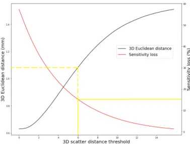
Fig. 5. Mean 3D Euclidean distance and event loss when all events scattered beyond the distance threshold are discarded.

separability is greatly enhanced, as the AUC increases to 96%. From this point, we explored two approaches to improve po-sitioning while maintaining high sensitivity standards. Either, far-scattered and close-or-non-scattered are positioned by sepa-rate positioning models. Or, the far-scattered events are rejected. Alas, the two independent positioning models do not signifi-cantly improve positioning. Whereas the far-scattered events reached a mean absolute x-, y- or DOI-bias of about 2mm in the original 2D+DOI positioning model, the separate far-scattered positioning model reaches 1.8mm. The close-or-non-scattered positioning model reaches a mean 3D Euclidean distance of 1.07mm. The second approach involves discarding far-scattered events. Figure 5 shows what happens to the 3D Euclidean dis-tance and the event loss when all events that scattered beyond the threshold are discarded from the test dataset. A threshold of 6mm signifies a 3D Euclidean distance reduction from 1.53mm to 1.08mm at the cost of a 15% event loss. Figure 5 does not yet take into account the imperfect accuracy of the scattering distance classification model (i.e. 92%). Table III lists the per-formance values of the 2D+DOI positioning model when it only positions events that were classified as close-or-non-scattered by the classification model.

TABLE III

POSITIONING PERFORMANCE AFTER REJECTION OF FAR-SCATTERED EVENTS(VALUES IN MM).

Mean & median FWHM 0.375 & 0.368 Mean absolute x- or y-bias 0.45

Mean absolute DOI-bias 0.71

3D Euclidean distance 0.95

In an experimental setup there is a lack of DOI and Compton scatter ground truth. Borghi, G., et al. [3] propose a practi-cal method for acquiring DOI knowledge experimentally. To our knowledge, no research has been devoted to deriving exper-imental scatter ground truth. Preferably we would not want to further complicate the design and calibration by adding more

read-outs. In the end, we only want to improve the spatial res-olution. We therefore propose to apply the strategy of rejecting far-scattered events in an experimental setup, with the distance classification model trained on simulated data and the position-ing model trained on either simulated or experimental data. If the spatial resolution improves, all the better. If it does not, dif-ferent approaches should be explored. If simulation is in close agreement with reality there is no reason for the scatter distance classification model to perform worse on experimental data.

IV. CONCLUSIONS

Neural networks of sufficient complexity are very suitable candidates for γ-positioning. We reached a resolution in FWHM of 0.4mm, a mean absolute x- and y-bias of 0.7mm and mean ab-solute DOI-bias of 0.9mm. Both a 3D positioning model and the combination of a 2D positioning model and a DOI estimation model yielded similar results. The degrading effect of Compton interactions on the positioning performance was observed, espe-cially in the broadening of the prediction or bias distributions’ tails. The mean absolute DOI bias was reduced to 0.47mm when excluding Compton interactions, the 2D positioning error from 1.08mm to 0.36mm. However, excluding 60% of all events is unacceptable considering the already challenging sensitivity of PET systems. To address the resolution-sensitivity trade-off a scattering distance threshold was proposed to classify events. A scattering distance classification model responsible for sepa-rating far-scattered from close-or-non-scattered reached an ac-curacy of 92%. Far-scattered events were rejected from posi-tioning, because of their poor positioning performance. For a 15% event loss (i.e. scatter distance threshold of 6mm) the 3D Euclidean distance was improved from 1.53mm to 0.95mm. To our knowledge this is the first proposed strategy for dealing with Compton interactions in monolithic crystals. Future research could extend this approach to an experimental setup. Efforts are currently being made at the MEDISIP lab and results are soon to follow. The challenge of acquiring scatter ground truth de-serves attention. Future studies could also aim to investigate a range of photon incidence angles, as this likely influences the relation between interaction position and light distribution. We also propose to further investigate the influence of the scattering angle on the positioning performance. The scattering distance in the z-direction more seriously affects the DOI-bias, while the 2D scattering distance has more impact on 2D positioning.

REFERENCES

[1] Stockhoff, Mariele, Roel Van Holen, and Stefaan Vandenberghe. ”Optical simulation study on the spatial resolution of a thick monolithic PET detec-tor.” Physics in Medicine Biology 64.19 (2019): 195003.

[2] Babiano, Victor, et al. ”-Ray position reconstruction in large monolithic LaCl3 (Ce) crystals with SiPM readout.” Nuclear Instruments and Methods in Physics Research Section A: Accelerators, Spectrometers, Detectors and Associated Equipment 931 (2019): 1-22.

[3] Iborra, A., et al. ”Ensemble of neural networks for 3D position estimation in monolithic PET detectors.” Physics in Medicine Biology 64.19 (2019): 195010.

[4] Borghi, Giacomo, Valerio Tabacchini, and Dennis R. Schaart. ”Towards monolithic scintillator based TOF-PET systems: practical methods for detector calibration and operation.” Physics in Medicine Biology 61.13 (2016): 4904.

[5] Wang, Y., et al. ”3D position estimation using an artificial neural network for a continuous scintillator PET detector.” Physics in Medicine Biology 58.5 (2013): 1375.

(12)

[6] Berg, Eric, and Simon R. Cherry. ”Innovations in instrumentation for positron emission tomography.” Seminars in nuclear medicine. Vol. 48. No. 4. WB Saunders, 2018.

[7] M¨uller, Florian, et al. ”A novel DOI positioning algorithm for monolithic scintillator crystals in PET based on gradient tree boosting.” IEEE Transac-tions on Radiation and Plasma Medical Sciences 3.4 (2018): 465-474. [8] Decuyper, Milan, Mariele Stockhoff, and Roel Van Holen. ”Deep Learning

for Positioning of Gamma Interactions in Monolithic PET Detectors.” IEEE NSS-MIC 2019. 2019.

[9] Yang, Ting-Yi. ”Machine learning for high resolution 3D positioning of gamma-interaction in monolithic PET detectors” (2019).

[10] Babiano, Victor, et al. ”-Ray position reconstruction in large monolithic LaCl3 (Ce) crystals with SiPM readout.” Nuclear Instruments and Methods in Physics Research Section A: Accelerators, Spectrometers, Detectors and Associated Equipment 931 (2019): 1-22.

[11] Peng, Peng, et al. ”Compton PET: A simulation study for a PET module with novel geometry and machine learning for position decoding.” Biomed-ical Physics Engineering Express 5.1 (2018): 015018.

[12] Li, Xiaoli, et al. ”A high resolution, monolithic crystal, PET/MRI detec-tor with DOI positioning capability.” 2008 30th Annual International Con-ference of the IEEE Engineering in Medicine and Biology Society. IEEE, 2008.

[13] Benlloch, Jos´e M., et al. ”The MINDVIEW project: First results.” Euro-pean Psychiatry 50 (2018): 21-27.

(13)

List of Figures

1.1 Pixelated versus monolithic scintillation detector [1]. . . 9

1.2 Relative occurrence of number of Compton interactions for a 50x50x16mm3 _{LYSO crystal. 10} 1.3 Illustration of different interactions and their influence on the light distribution. Because of the Compton interaction’s small light yield it is often hardly discernible within the photoelectric signal. . . 11

2.1 Diagram of the sampled light distribution at two different interaction coordinates [49]. (a) Interaction at the crystal’s center. (b) Interaction near a corner, demonstrating truncation at the edges. . . 17

2.2 Compton scattering mechanism illustrating the scattering angles. . . 18

2.3 x (left) and DOI (right) positioning error at one test position including (blue) and exclud-ing (red) scattered events [13]. . . 19

2.4 Illustration of optical barriers in a scintillator slab with edge readout (left) and how it creates shade to increase variance in the SiPMs’ signal (right) [45]. . . 21

3.1 Brain scan in MRI (left panel), PET (right panel) and fused to integrate both anatomical and physiologic information in PET-MRI (middle panel) [56]. . . 23

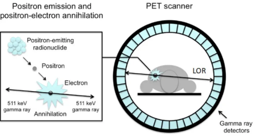
3.2 Schematic representation of positron emission and positron-electron annihilation (left), and PET-scan setup (right) . . . 25

3.3 Schematic representation of pixelated (left) and monolithic (right) scintillator coupled to SiPM photosensors [1]. In monolithic detectors spatial resolution is not limited by pixel size. Furthermore, monolithic detectors provide information about the DOI. . . 26

3.4 Schematic representation of parallax effect, i.e. how lack of DOI knowledge affects LOR reconstruction. . . 27

3.5 Types of coincidence measurements. From left to right: true coincidence, random coinci-dence and scattered coincicoinci-dence. . . 28

3.6 Three primary gamma ray interaction mechanisms with matter. . . 29

3.7 Predominant mode of gamma interaction as a function of photon energy and absorber’s Z [61]. . . 30

3.8 Probability density function deduced from the Klein-Nishina formula versus scattering angle for several incoming photon energies [57]. . . 30

4.1 Example of under-, over- and appropriate fitting [72]. . . 33

4.2 Representation of an artificial neuron [73]. . . 35

4.3 The three most common activation functions [74]. . . 35

4.4 Feedforward neural network with 2 hidden layers [23]. . . 36

4.5 Recurrent Neural Network that feeds its output back into the hidden layer [75]. . . 37

4.6 Example of the typical learning curve corresponding to an underfitting (left) and overfit-ting (right) model. . . 40

5.1 Illustration of the calibration of a 50x50x16mm3 _{L(Y)SO crystal, backed by a 8x8 SiPM} array with pixel size 6x6mm2 _{[10]. . . 42}

5.2 Example of 2 signals at equal (x,y) interaction position, but differing in DOI. Channels 1-8 correspond to the summed x-pixels, 1-16 to the summed y-pixels. . . 43

5.3 Illustration of sensitivity and specificity [78]. . . 51

5.4 Illustration of limited separability of predicted classes [77]. The decision threshold is varied to obtain appropriate sensitivity or specificity. . . 51

6.1 Loss (left) and bias (right) learning curves for 2D positioning model. . . 52

(16)

6.3 Histogram with prediction distributions for every calibration position. The green dots represent the actual calibration positions. . . 55 6.4 Influence of scattered events on the x-bias distribution. . . 55 6.5 Histogram of 2D predictions on 1mm spaced grid in between the calibration positions (i.e.

[-4.5, 4.5] x [-4.5,4.5]). . . 57 6.6 Histogram of 2D predictions on flood source data, containing 500x500 bins each with an

average number of 3.4 ± 2 events. . . 58 6.7 Loss or MSE (left) and bias or MAE (right) learning curve for DOI estimation model.

Loss is not simply bias squared, because squaring and averaging are not commutative. . 58 6.8 2D histogram of the Mean Absolute Error (MAE) on the DOI estimation. . . 59 6.9 Variation of the MAE (left) and Bias (right) with depth (i.e. 0mm is located at the

bottom, near the photosensors). . . 59 6.10 Influence of scattered events on the DOI-bias distribution. . . 60 6.11 Goodness-of-fit for the 2D prediction distribution across the detector plane. . . 61 6.12 Prediction distributions fitted to a Gaussian at two distinct calibration positions: (a)

‘good’ fit at the center, (b) truncated at the edge . . . 61 6.13 The mean absolute x-bias (left) and mean absolute DOI bias (right) versus three ranges of

scattering distance. The bins ]0,2[, [2,6[ and [6,40[ each contain one third of all scattered data. The far scattered photons are more poorly positioned by the 2D+DOI positioning model. . . 62 6.14 Example of 3 signals with equal first interaction position (x=0, y=6 and z=10), but

different scattering interactions. The non-scattered signal (black) is hardly distinguishable from the close-scattered signal (green). On the other hand, there is very little evidence of the first (Compton) interaction of the far-scattered (yellow) signal. Therefore, it would be hardly distinguishable from a signal caused by a non-scattered photon that interacts photoelectrically at a position nearby. . . 63 6.15 Mean 3D Euclidean distance and event loss when all events scattered beyond the distance

threshold are discarded. . . 64 6.16 Influence of far-scattered events on the x- and DOI-bias distribution. . . 65 6.17 Illustration of influence of scattering direction on the resulting light distribution. . . 66

(17)

List of Tables

2.1 Methodology and performance overview of research on positioning in monolithic PET detectors. Calibration data was either acquired experimentally (Exp) or through simulation. 15

5.1 Hyperparameters and specifications of the 2D positioning model. . . 45

5.2 Hyperparameters and specifications of the DOI estimation model. . . 45

5.3 Hyperparameters and specifications of the 3D positioning model. . . 46

5.4 Hyperparameters and specifications of the scattering identification model. . . 46

5.5 Hyperparameters and specifications of the scattering distance classification model. . . 47

5.6 Hyperparameters and specifications of the 3D positioning model for far scattered photons (i.e. scattering distance > 6mm). . . 48

5.7 Hyperparameters and specifications of the 3D positioning model for close-or-non-scattered photons (i.e. scattering distance < 6mm, or not scattered at all). . . 48

6.1 2D positioning performance at the 5x5mm2 _{center region vs. 3mm edge strip (all values} in mm). . . 53

6.2 2D positioning performance (all values in mm). . . 56

6.3 Comparison of the 2D positioning performance for 1mm- and 0.25mm-spaced test data in the 5x5mm2 _{center region. The calibration positions were excluded from the} 0.25mm-spaced grid. . . 56

6.4 Comparison of the direct 3D positioning model and the 2D+DOI model (all values in mm). 60 6.5 Test performance of the scattering identification model. . . 62

6.6 Test performance of the scattering distance classification model. . . 64

6.7 Performance of 2D+DOI positioning model when rejecting events that were classified as far-scattered by the scattering distance classification model (all values in mm). . . 65

(18)

List of Abbreviations

(A)NN (Artificial) Neural Network

AUC Area Under Curve

CNN Convolutional Neural Network

CT Computed Tomography

DOI Depth of Interaction

DSR Dual-sided readout

FOV Field of View

FWHM Full Width at Half Maximum

FWTM Full Width at Tenth Maximum

GTB Gradient Tree Boosting

kNN k Nearest Neighbor

MAE Mean Absolute Error

MRI Magnetic Resonance Imaging

MSE Mean Squared Error

LOR Line of Response

ROC Receiver Operating Characteristics

SGD Stochastic Gradient Descent

SiPM Silicon Photomultiplier

SPECT Single Photon Emission Computed Tomography

(19)

(20)

1

Introduction

1.1 Problem Statement

Positron Emission Tomography (PET) is a functional medical imaging modality that is most commonly used for the detection and follow-up of tumors. Currently, the main limiting factor for the spatial resolution is the scintillation detector. The scintillators are positioned in a ring around the patient and are responsible for the detection of two coincident photons that originate from a positron-electron annihilation inside the patient. Most clinical PET-scanners today are equipped with pixelated detectors consisting of many long and thin crystals. As such, positioning a scintillation event simply consists of identifying the fired pixel. In that case, the spatial resolution remains limited to the pixel size (cfr. Figure 1.1). Furthermore, there is no information on the Depth of Interaction (DOI) within the pixel.

Figure 1.1: Pixelated versus monolithic scintillation detector [1].

Monolithic scintillators are considered promising alternatives to pixelated detectors in the context of small object PET imaging, e.g. brain, pediatric or small animal imaging, and in TOF-PETs. They exhibit superior spatial resolution as well as other desirable qualities such as good energy and time reso-lution, high sensitivity and lower cost. However, as opposed to pixelated detectors, there is no direct way of positioning a photon interaction in a continuous crystal. Plentiful specialized positioning algorithms have been proposed throughout the years. They are all based on the causal relationship between the scintillation location and the light distribution that is measured by an array of photosensors at the back-side. There is an ongoing search for the most efficient and accurate positioning algorithm. Statistical based positioning algorithms such as Maximum Likelihood estimation [4], machine learning algorithms such as k Nearest Neighbor [8] and non-linear analytical models [11] reach high spatial resolution, but often at a very large computational cost and requiring intricate procedures for DOI encoding. Progress in computing power has enabled the use of Artificial Neural Networks (ANNs) for the sake of positioning and pattern recognition. ANNs are fast and parallelizable, and have proven to yield sub-mm 2D spatial resolution ([1],[16]). Moreover, they are capable of estimating DOI directly, which is of paramount

(21)

impor-tance in the reduction of parallax error and in the further development of TOF-PET systems. Effective DOI encoding also allows thicker crystals to be used, which increases γ-photon detection efficiency, thus sensitivity. Furthermore, in a 3D PET system with accurate DOI decoding, it is possible to use a larger number of detector rings, i.e. a longer axial field of view (FOV) [62].

Research has indeed proven ANNs to be effective DOI estimators ([1],[5],[6]), however there is still work to be done. At 511keV photoelectric interactions are not the only γ-interactions to take into account. A large fraction of photons undergo one or multiple Compton interactions within the crystal. In the case of a 50x50x16mm3 _{LYSO crystal the relative occurrence of the amount of Compton interactions is}

displayed in Figure 1.2. About 60% of all γ-photons undergo at least one Compton interaction.

Figure 1.2: Relative occurrence of number of Compton interactions for a 50x50x16mm3 _{LYSO crystal.}

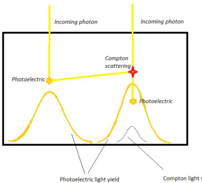
A Compton interaction occurs when a photon is scattered by an electron in the crystal lattice. Depending on the scattering angle an amount of energy is transferred from photon to electron. The electron relaxes by emitting the energy in the form of light. The light yield from a Compton interaction is small in comparison to that of a photoelectric interaction (i.e. photon absorption), because of the smaller energy deposition. The first interaction position is the only relevant one to consider in the reconstruction of the Line of Response (LOR). Hence, in the case of Compton scattering, positioning algorithms should be able to discern the small Compton light yield within the light yield caused by the final photoelectric interaction (cfr. Figure 6.14). This is a serious complication to the positioning problem. Compton scattered photons degrade spatial resolution and introduce a blurring in the final image. The degrading effect of intracrystal Compton scattering is mentioned in many relevant studies, but a study that effectively tackles the problem has, to our knowledge, yet to be published.

(22)

Figure 1.3: Illustration of different interactions and their influence on the light distribution. Because of the Compton interaction’s small light yield it is often hardly discernible within the photoelectric signal.

1.2 Objectives and Research Question

The challenges that were mentioned in the problem statement can be summarized in the following research questions:

• How well-equipped are Neural Networks in the positioning of γ-interactions within monolithic PET detectors, in both (x,y) interaction coordinates as in DOI?

• How do Compton scattering interactions affect the positioning performance? • How could this degrading effect be mediated?

The final question raises an important trade-off to be made. On the one hand, we would not wish to see the spatial resolution degraded by Compton scattering interactions. On the other, Compton scattered photons make up a large part of all detected photons and we would not wish to compromise sensitivity, an already fragile parameter of PET systems.

It could be stimulating to set concrete objectives. Based on previous research in our group it is not overly ambitious to expect a resolution in FWHM of less than 0.5mm ([1],[16]) and sub-mm mean ab-solute x-, y- and DOI-bias, when working with simulation data. Working with experimental data we expect a degradation due to several reasons including: crystal imperfections, calibration beam diameter, light entering the crystal [10] and many more noise inducing non-idealities. The quality of data is of direct influence to the performance of Neural Networks.

With regards to Compton scattering in monolithic, single-sided readout detectors, to our knowledge no strategy has been proposed in the literature. In general, Compton scattered events are treated in no different way than non-scattered events.

(23)

1.3 Thesis Outline

The dissertation comprises seven chapters, including this introductory chapter. The literature analysis of chapter 2 aims to familiarize the reader with existing, relevant research. A variety of approaches and recent advances are discussed to shape a clear view on where this work might contribute. Chapters 3 and 4 provide a solid background on the topics of interest: PET imaging and Neural Networks. Chapter 5 unveils the materials and methods that were used to carry out the research and meet the objectives. It discusses data gathering and handling, and Neural Network training. Furthermore, a thorough overview of all trained models is presented. The chapter is concluded with definitions of the measures that will evaluate the models’ performance. Chapter 6 finally presents and elaborates on the results of the investigation. The findings are summarized in chapter 7.

(24)

2

Literature Analysis

2.1 Review of Related Research

In order to gain a clear perspective on the work that has been done in the field of gamma positioning in monolithic PET detectors and on where this work might add its contribution, a literature analysis is indispensable. A variety of positioning algorithms are discussed and evaluated, before zooming into the algorithm of our interest: Artificial Neural Networks. Of particular interest as well is the role of Compton scattering on the positioning performance.

2.1.1 Positioning algorithms

Several methods to extract spatial information from a monolithic scintillator have been proposed in the past. It all started with the centroid method (i.e. Anger logic), in which the incident gamma posi-tion was directly calculated as the weighted sum of the pixel posiposi-tions, with the weights given by the signal amplitudes in each pixel. It is commonly implemented by means of a resistor-network, which also provides some sensitivity for DOI estimation. The method was first proposed for the purpose of scintillation cameras in 1958 [48]. The Anger method usually only works in the detector’s center and is now widely considered too simple to capture the complicated relation between the light distribution and the interaction position. Moreover, there is no way of taking into account scattering information [2]. Attempts have also been made to capture this complex relation in non-linear analytical models. Li, Z., et al. [15] construct a function that maps the scintillation light point-of-origin to the measured photosensor pixel signals in monolithic scintillation crystals. Three sources of scintillation photons are distinguished: 1) photons emitted directly towards the photosensors at the bottom, 2) photons that undergo mirror-like reflection at one of the crystal’s faces and 3) photons that undergo diffuse reflection at the crystal’s faces. The latter photons re-enter the crystal at a random angle, thus losing all spatial information and contributing only to the background signal. The light collected in a pixel is the sum of these 3 contributions. The terms are calculated based on the assumption that the number of detected photons in a pixel is proportional to the solid angle subtended by that pixel seen from the source lo-cation. The model’s parameters are determined by least-squares fitting the three term equation to the light detected by each pixel of the SiPM array. Using this exact same analytical model Etxebeste, A., et al.[11] reached an average (x,y)- and DOI resolution of 1.2mm and 2mm respectively. Compton scattered photons are not included in the theoretical model. In that same study it was observed that scattered events degrade the DOI resolution from 1.6mm to 2mm.

One should bear in mind that analytical models, because of their generally complicated nature and lengthy minimization calculations, are not very suitable to provide real-time estimations [62]. In addi-tion, the theoretical model does not include experimental set-up particularities such as inhomogeneities

(25)

in the crystal or in the optical coupling to the photosensors, etc.

The statistics based positioning (SBP) methods rely on comparing the detector’s response with a refer-ence data set. The referrefer-ence data set consists of a number of recorded or simulated light distributions at known interaction position.

An example of such an approach is based on the calculation of the likelihood function [4]. If we assume that all light distributions follow a normal distribution, the likelihood function describes the probability of observing a certain normal light distribution given the scintillation position. The Maximum Like-lihood estimate is the scintillation position most likely to cause the observed light distribution. This position estimate is calculated by means of look-up tables (LUT), usually corresponding to the mean and standard deviation of the light probability density function versus the (x,y) position. The most basic maximum likelihood procedure only provides 2D information. However, Miyaoka, R., et al. [4] were able to estimate the DOI with this approach as well, by extending it with a clustering method. The detector was divided in 7 depth layers and 2D LUTs were created for each layer. A neat trick was then applied to increase the DOI resolution, which was now intrinsically limited by the layer width: based on the 7 DOI LUTs, a third-order polynomial was fit to the mean and variance for each (x,y) position. Then, 15 DOI LUTs were generated from the fit. In that manner, already back in 2008, the authors impressively reached an (x,y)-resolution in FWHM of 0.83mm and a DOI resolution of 1.83mm.

Machine learning algorithms make up a large portion of high performing positioning algorithms, ex-amples being the k Nearest Neighbor (kNN) and the Gradient Tree Boosting (GTB) algorithm. The kNN algorithm was first proposed for position decoding by Maas et al. [55] in 2006, and more were quick to follow [8],[9],[10]. However, the kNN algorithm is computationally demanding in both memory and time, because the distance metric has to be computed for all events and reference distributions. Borghi, G., et al. [8] propose a more efficient approach: accelerated kNN. It relies on a fast position estimation before performing the kNN algorithm on a much smaller reference dataset. Position pre-estimation is obtained through calculation of position related parameters of the light distribution: the center of gravity for 2D positioning and the sum of squared pixel intensities for DOI estimation. By dividing the crystal in regions LUTs are created for every parameter and only a small fraction of the reference dataset is selected for more precise positioning by the kNN algorithm.

The GTB algorithm [3] in itself is more computationally efficient as it is organized as an independently evaluable set of chains of binary decisions (decision trees).

An algorithm of particular interest in the machine learning family is the Artificial Neural Network (ANN), the method that will be employed in this work. They require a larger database. However the advantages of using an ANN for gamma positioning in monolithic detectors are plentiful: 1) Once an ANN is trained, it provides a direct, real time estimation for any event. 2) The estimated position is continuous over the entire crystal. 3) ANNs are universal approximators, meaning they are capable of approximating any measurable function to any desired degree of accuracy. They are able to directly ex-tract and learn 3D information and very importantly, they can include the effect of Compton scattering. In De Acilu, P., et al [2] comparing the Anger logic based, statistics based, kNN and ANN method the ANN emerged as the clear winner in terms of spatial resolution, beating the kNN algorithm by 40%. Studies by M. Stockhoff et al. [10] and TY Yang [1] allow a direct comparison between the kNN and the ANN approach, as they employed the exact same setup and method of data acquisition. Once again, the ANN takes the lead with an average FWHM of 0.46mm versus 0.56mm for kNN. Indeed this is confirmed by Decuyper, M., et al. [16]: “We showed that based on the same dataset, deep neural networks can achieve a better spatial resolution compared to a nearest neighbor positioning method, even with lower

(26)

number of training events.” Table 2.1 lists several studies, according to their data acquisition, positioning algorithm, and 2D- and DOI-resolution in FWHM. It is generally hard to compare studies because of the diversity in e.g. crystal size, experimental setup or simulation details, etc.

Data ac-quisition Algorithm Average x,y spatial resolution (FWHM in mm) Average DOI resolution (FWHM (or MAE) in mm)

TY Yang (2019) [1] GATEv8.0 ANN 0.46 0.74 (MAE)

V. Babiano et al. (2019) [52] Exp ANN 3.35 F. Hashimoto et al. (2019) [5] GEANT4 ANN 1.54 1.59

Y. Wang et al. (2013) [6] Exp ANN 1.86 2

P. Bruyndonckx et al. (2008) [7]

Exp ANN 1.6 /

Decuyper, Milan, et al. (2019) [16] GATEv8.0 ANN 0.23 / F. M¨uller et al. (2018b) [3] Exp GTB 1.86 2 M. Stockhoff et al. (2019) [10] GATEv8.0 kNN 0.56 1.6 (MAE)

G. Borghi et al. (2016) [8] Exp kNN 1.7 3.73

G. Borghi et al. (2016) [54]

Exp kNN 1.1 2.4

H. T. Van Dam et al. (2011b) [9] Exp kNN 3.2 3.4 X. Li et al. (2008) [4] DETECT2000 SBP 0.83 1.83 A. Etxebeste et al. (2016) [11] GATEv6.1 Analytical 1.2 2

Table 2.1: Methodology and performance overview of research on positioning in monolithic PET detec-tors. Calibration data was either acquired experimentally (Exp) or through simulation.

2.1.2 Neural Networks

The following paragraphs review works that specifically studied NNs for position decoding in monolithic scintillators. It can be instructive to know which NN hyperparameters proved successful in the past and how certain challenges were met.

In TY Yang’s work [1] a NN with two hidden layers of 128 nodes was trained to perform 2D gamma-interaction positioning for the exact same setup as in this work. Additional DOI estimation was only performed in the center region of the crystal. This surprisingly shallow NN reached an average 2D resolution and DOI MAE of 0.46mm and 0.74mm respectively. The DOI was estimated by means of a depth layer approach. The crystal is divided in 6 depth layers and a NN is trained to allocate the depth layer in which the interaction took place. The Mean Absolute Error (MAE) is calculated as the absolute difference between the center of the predicted depth layer and the true DOI. If truth be told, the depth

(27)

layer approach is unnecessary for DOI estimation by NNs. NNs are perfectly capable of estimating the DOI in a continuous manner, without being limited by the layer width. In this case, the layer approach was solely used to allow direct comparison with the kNN-algorithm [10]. A comparison which, as already mentioned, ruled in favor of NNs.

In Wang, Y., et al. [6] a global 2D NN is trained first. The detector plane is then divided in 35 equal squares. For each square an x-, a y- and a DOI-estimating NN is trained separately. Every event goes through a processing chain: the global 2D NN positions the event in the plane and assigns it to one of 35 cuboids. Ultimately, the x-, y- and DOI NNs responsible for the assigned cuboid estimate the 3D position within the cuboid. The abundance of NNs to be trained is compensated by a) their simplicity (2 hidden layers of 8 neurons) and b) appropriate use of detector symmetry.

In every reviewed work it was observed that the estimation error (=bias) becomes worse at the edge area of the detector for 2D estimation. At the edges the NN tends to shift events towards the center (edge effect). Wang, Y., et al. [6] thereto propose an edge bias correction. All events that the global NN assigns to cuboids at the edges receive a bias correction. This is only possible because of their choice to train a global NN that feeds sectional NNs. If there is one global NN to cover the whole detector there is no way of knowing a priori where the event took place, hence there is no way of correcting the edge bias.

A different detector design such as a single, tube-like scintillator eliminates all the edges and consequent edge effects, but is significantly more expensive [58].

Iborra, A., et al. [14] propose a different scheme: an ensemble of NNs. They argue that different detectors (or sectors of a detector) of the same design might have differences in optical coupling, pho-tosensor response, etc, affecting their output. When only a single NN is used this variability in light distribution may introduce inter- and intra-detector variability in the predictions. Hence, an ensemble of NNs is employed, a method known to reduce variability in predictions. Several networks, differing in number of layers and units only, were trained and tested. The ensemble average of the 10 best performing networks was taken as the final position estimate. The three interaction coordinates (x,y,z) were esti-mated by separate network ensembles. The search space for the number of hidden layers h and number of units per layer n: h=(2,3,4,5,6) and n=(100,200,400). The best performing NN architecture was one made up of 6 layers and an average number of total nodes of 1400 reaching a FWHM of 2mm at best. Four detector designs were simulated, each having their own light absorbing coating or teflon wrapping to decrease or increase inner reflections. Reflective coatings increase the energy resolution. However, increasing inner reflections has a negative impact on the positioning accuracy for methods that rely on centrality and dispersion functions such as statistics based positioning. NNs on the other hand can take advantage of the extra information inner reflections provide, especially for interactions at the edges. Once again, there is a systematic error in the 2D-positioning at the edges because of the truncated light distribution (Figure 2.1). Degradation of the DOI resolution at the bottom of the crystal is an issue as well, which the authors attribute to scintillation light sampling. When scintillation takes place close to a photosensor almost all light is detected by that sensor thus limiting the variance and the ability of the NN to infer information.

In Decuyper, M., et al. [16] an ANN was trained using the exact same setup and data acquisition as in this work. The network weights were optimized through backpropagation using stochastic gradient descent with Nesterov momentum 0.9, a mini-batch size of 256 and an initial learning rate of 10−3_.

(28)

Figure 2.1: Diagram of the sampled light distribution at two different interaction coordinates [49]. (a) Interaction at the crystal’s center. (b) Interaction near a corner, demonstrating truncation at the edges.

networks (>3 layers of 256 neurons) as the network begins to overfit. At that point, only increasing the number of training events can improve performance. The best performance was obtained in a neural network with four hidden layers of 512 neurons and 8000 training events per position. As such a 2D FWHM of 0.23mm was attained, a result so far unsurpassed in research. The authors conclude that a very high resolution can be obtained with enough training data and a complex network. As for the event processing rate, no less than 10 million events can be positioned per second.

In studies on gamma-positioning in a monolithic LaCl3(Ce) crystal [52],[53] the authors report

no-tably better results when using three independent models for x-, y- and z-positioning instead of a single network with three outputs. Then again, they trained a relatively simple NN containing only one hidden layer of 64 neurons. They reached a 2D FWHM of 3.35mm, which is not bad, considering it was attained in an experimental setup.

DOI estimation in an experimental setup is not a picnic. Most calibration setups are only designed to perpendicularly irradiate the top of the crystal. When calibrating the detector from the top (i.e. at known (x,y)) there is no direct way of knowing the DOI. Babiano, V., et al. propose a phenomenological approach by assuming an inverse-linear relationship between DOI and the cross-section of the light distri-bution at half maximum. They compared their findings to a Monte Carlo simulation with 5mm FWHM broadening and found reasonable agreement. Hence, they attained an uncertainty on the experimental DOI, in other words a DOI resolution in FWHM, of 5mm.

Another approach to the problem of experimental DOI calibration is to irradiate the crystal from the side (i.e. at known depth). However, when the crystal is too thick very little photons would reach the other side due to absorption. Therefore, the opposite side would have to be irradiated as well, requiring an even more complicated setup and lengthy calibration procedure.

Alternatively, as in this work, a NN trained on simulation data could perform DOI estimation. 2.1.3 Compton Scattering

One of the main objectives of this work is to investigate the effect of Compton scattered events on the positioning accuracy in monolithic detectors. As of now, there is little research that focuses solely on this challenge. In most of the literature on position decoding the degrading effect of Compton interactions is mentioned, sometimes quantified, but not effectively tackled.

(29)

Figure 2.2: Compton scattering mechanism illustrating the scattering angles.

Research agrees that the DOI resolution is degraded more than the (x,y)-resolution since small an-gle scattering is preferred (cfr. Section 3.3). Small anan-gle or forward scattering refers to the situation of small angle φ in Figure 2.2. In the case of perpendicular irradiation from above the scintillation crystal, forward scattering is directed towards the photosensors at the bottom. When a photon scatters forward, very little energy is transferred from the photon to the recoil electron. This causes the scattered event to be nearly indiscernible from the light distribution of a non-scattered event that scintillated at the same location. Ultimately, this has an impact on the DOI estimation, and consequently, the time-of-flight (TOF) calculation. The influence on TOF increases with the scattered distance. Meanwhile, the Line of Response (LOR) is only slightly affected by small angle scattering.

Average detector response based methods like SBP and kNN don’t take into account Compton scat-tering. One possible approach consists of discarding scattered events. However this would signify a 60% event detection loss. Most often, scattered events are not treated in any different way than non-scattered events. Hence, there is no sensitivity loss, however significant resolution loss is inevitable. In [13] for instance, which employs Maximum Likelihood estimation, the authors report that by excluding scat-tered events from the test data the (x,y)-resolution is improved by 8% (from 0.86mm to 0.8mm) and the DOI resolution by 16% (from 1.19mm to 1.05mm). Figure 2.3 is representative for how including scattered events broadens the x positioning error distribution, hence increasing FWHM, and leads to a more pronounced tail in DOI estimation. This means that scattered events were positioned closer to the photodetectors, while in fact the first interaction took place higher up in the crystal. Evidently, our interest goes exclusively to the first interaction location as it is the only relevant position for Line of Response reconstruction.

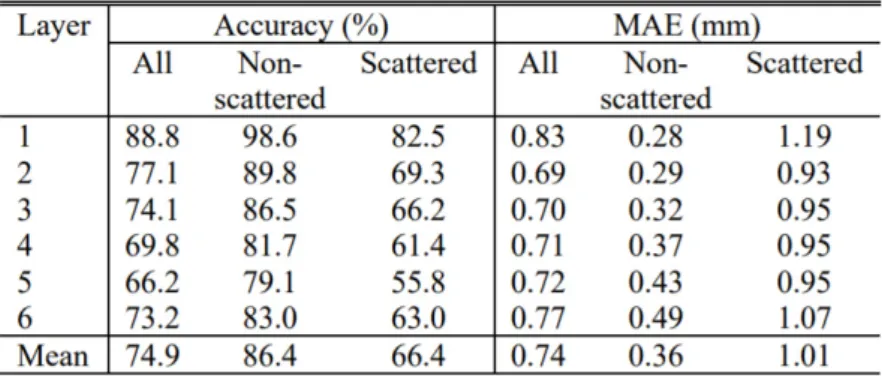
NNs on the other hand are universal approximators, which in theory enables them to incorporate Comp-ton scattering. In the work of T.Y. Yang [1] we find following table with the DOI accuracy and MAE in 6 depth layers (layer 6 is closest to the photosensors). What stands out is the superior DOI estimation of non-scattered versus scattered events, proving yet again the potential of this investigation. Noteworthy as well is the degradation in accuracy towards the photosensors. In part this can be attributed to the attenuation of photons. Therefore less training data is available at increasing depth. If training data is imbalanced and not sampled proportionally, it could be that the NN superficially learns to underestimate the DOI simply because a small DOI is more prevalent in training. Correction of the data imbalance by sampling according to the attenuation function, could potentially improve the DOI resolution. How-ever, correcting for imbalanced data in regression problems is more tricky than in classification problems

(30)

Figure 2.3: x (left) and DOI (right) positioning error at one test position including (blue) and excluding (red) scattered events [13].

(31)

and less research is available on the topic. One proposed technique is called Synthetic Minority Over-Sampling Technique (SMOTE) for Regression [63]. Another explanation for degraded DOI resolution with depth is the increasing number of Compton interactions.

Table 2: DOI accuracy and MAE for scattered and non-scattered events in all 6 depth layers. Iborra, A., et al. [14] make following comments on Compton scattering. At first, scattered and non-scattered events were tested together, leading to poor results in the positioning of the first inter-action (Compton or photoelectric). It was observed that only the first interinter-action events which were photoelectric in nature were positioned properly. Attempts at training classification networks aimed to separate events that included one or more Compton interactions from those that were solely photoelectric remained unsuccessful. Deviations in the collected light for events that shared approximately the same photoelectric location (but that could have been Compton scattered before) were weak in magnitude. In other words, the light yield from Compton scattering was snowed under by the photoelectric interaction and remained undetectable by the NN. The authors did not discard scattered events. However, through-out the entire paper, the photoelectric interaction was assumed to be the first interaction position, and consequently, the NN was trained to estimate the photoelectric interaction position. As such, the bias between predicted photoelectric interaction position and true first interaction position was partly deter-mined by the scattering distance.

So it seems that separating scattered from non-scattered events is difficult, even for NNs. There is no mention of this issue in other studies on monolithic PET detectors, therefore we take a look at gamma cameras, also called Anger or scintillation cameras, which use scintillation to form a 2D image of high energy X-rays and are part of most SPECT systems today. Indeed, a study on gamma cameras [52] suggests that scattered events with a small scattering distance are nearly indistinguishable from non-scattered events. Their solution is to place photodetectors on top of the crystal as well (dual-sided readout (DSR)). As a direct comparison between the DSR [54] and single-sided readout [8] learns, the DSR configuration improves not only DOI estimation but 2D positioning as well. There is no mention of whether improved separability of scattered and non-scattered events lies at the root of that performance enhancement. We do know that monolithic scintillators in DSR configuration can be made relatively thick, hence increasing photon detection efficiency, without deteriorating DOI performance.

Some research [44],[45],[46] is devoted to exploring a layered detector design, in which crystal slabs are stacked in radial direction and read out by photosensors located at the four sides (edge readout). The slabs are separated by reflective films to maximize the number of photons reaching the sensors. The edge readout per layer allows for direct DOI-estimation, with a resolution limited by layer thickness. The measured light distribution at the edges is used to reconstruct the entire light distribution in the detector plane by means of the Mean-Detector-Response Function, which in its turn results from Monte Carlo simulations. Reconstructing a 2D light distribution allows the use of algorithms devoted to visual