Calculation and Mapping of Critical Thresholds in Europe:
Status Report 1999
Edited by:
Maximilian Posch
Peter A.M. de Smet
Jean-Paul Hettelingh
Robert J. Downing
Coordination Center for Effects
National Institute of Public Health and the Environment
Bilthoven, Netherlands
RIVM Report No. 259101009
Acknowledgments
The calculation methods and resulting maps contained in this report are the product of collaboration within the Effects Programme of the UN/ECE Convention on Long-range Transboundary Air Pollution, involving many individuals and institutions throughout Europe. The various National Focal Centers whose reports on their respective mapping activities appear in Part III are gratefully acknowledged for their contributions to this work.
In addition, the Coordination Center for Effects thanks the following:
•
The Air and Energy Directorate of the Dutch Ministry of Housing, Spatial Planning and the Environment for its continued support.•
The EMEP Meteorological Synthesizing Centre-West for providing the European deposition and ozone concentration data.•
The UN/ECE Working Group on Effects, and the Task Forces on Mapping and on Integrated Assessment Modelling, for their collaboration and assistance.•
The RIVM graphics department for its assistance in producing this report.Table of Contents
Acknowledgments
. . . .iiPreface
. . . .1PART I. Status of Maps and Methods
1. Critical Loads and their Exceedances in Europe: An Overview. . . .32. Summary of National Data. . . .13
3. Defining an Exceedance Function. . . .29
PART II. Related Research
. . . .33UK Help-in-Kind to the Mapping Programme. . . .35
Estimating the Exceedance of Critical Loads by Accounting for Local Variability in Deposition. . . .45
PART III. National Focal Center Reports
. . . .53Austria. . . .55 Belarus. . . .57 Belgium. . . .61 Bulgaria. . . .67 Croatia. . . .71 Czech Republic. . . .75 Denmark. . . .76 Estonia. . . .79 Finland. . . .81 France. . . .86 Germany. . . .91 Hungary. . . .97 Ireland. . . .102 Italy. . . .106 Netherlands. . . .111 Norway. . . .113 Poland. . . .119 Republic of Moldova. . . .124 Russian Federation. . . .127 Slovakia. . . .133 Spain. . . .139 Sweden. . . .140 Switzerland. . . .144 United Kingdom. . . .150
APPENDICES
A. The polar stereographic projection (EMEP grid). . . .155B. Some FORTRAN routines. . . .162
Preface
This report is the fifth in a biennial series prepared by the Coordination Center for Effects (CCE) to document progress made in calculating and mapping critical loads in Europe. The CCE, as part of the Mapping Programme under the UN/ECE Working Group on Effects (WGE), collects critical load data from individual countries and synthesizes them into European maps and data bases. These data bases, together with scientific advice on critical threshold methodologies, are provided to the integrated assessment modeling groups under the UN/ECE Working Group on Strategies (WGS). Via this route the effects-related work has a direct impact on the preparation of new protocols to the 1979 Convention on Long-range Transboundary Air Pollution. In particular, the critical loads data presented in this report, which have been formally approved by the WGE in August 1998, serve as input to the current negotiations of a “multi-pollutant, multi-effect” protocol.
The work of the CCE is carried out in close collaboration with an extensive network of national scientific
institutions (National Focal Centers) throughout Europe. At present, 24 National Focal Centers have provided critical loads data to the CCE, four more since the publication of the last Status Report in 1997. From modest beginnings in the early 1990s, we have reached a state where most of Europe is covered by national critical loads data. In addition to submitting data, National Focal Centers also participate in annual CCE Mapping
Workshops at which data and methodologies are reviewed.
As critical load and exceedance calculations become ever more complex, the issue of data transparency has become increasingly important over the last two years. Thus a mechanism has been set up by the WGE which gives parties the possibility to obtain critical loads data for work under the LRTAP Convention. In this context, it should also be noted that the CCE has made all data used in integrated assessment under the WGS available to National Focal Centers on CCE’s anonymous ftp server.
In addition, they were provided with a software tool (the “CCE Viewer”) which allows the user to quickly display and map the entire European critical loads data base. Data transparency also became more pressing after the Euro-pean Commission decided to use the EuroEuro-pean critical loads data in the formulation of an EU Acidification Strategy.
This report consists of three parts. Part I describes the present (1998) state of the critical loads data base used in UN/ECE negotiations. Chapter 1 gives an overview of the European critical loads and levels in the form of maps, and summarizes the methodology to calculate exceedances and their reductions by means of gap closures. The chapter is a stand-alone summary of the current state-of-the-art, and is designed to be understood also by the non-technical reader. Chapter 2 reports and analyzes in detail the critical loads and auxiliary data submitted by the National Focal Centers, and allows comparisons between countries. Chapter 3 explains the technical details of the so-called “accumulated exceedance” concept, which has been adopted in the integrated assessment of deposition reductions. Part II consists of two contributions: the first reports on UK help-in-kind to the Mapping Programme, and the second describes independent research on the uncertainties of exceedance calculations due to variations in deposition. Part III, the bulk of this report, consists of reports by the 24 National Focal Centers. They document the input data used to calculate national critical loads. Some of them also describe ongoing research carried out in the context of critical loads and levels. Finally, three appendices describe map projections, computer codes for exceedance calculations and conversion formulae for depositions and concentration units.
We hope that the 1999 CCE Status Report gives a fair overview of the accomplishments with respect to
European critical load calculations and mapping, but does not give the impression that nothing remains to be done.
The Editors
Introduction
As part of the Mapping Programme under the UN/ECE Working Group on Effects (WGE), the Coordination Center for Effects (CCE) collects critical load data from National Focal Centers (NFCs) and synthesizes them into European maps and data bases. The CCE also carries out exceedance calculations and assists in the development of the critical loads/levels methodology. Thus the purpose of this chapter is twofold:
(1) to summarize the definitions and concepts of critical loads and their exceedances in a non-technical manner with special emphasis on their use in European inte-grated assessment modeling carried out under the Long-range Transboundary Air Pollution (LRTAP) Convention and
(2) to present maps of critical loads and levels which are used in the current protocol negotiations.
1.1 Critical loads
For the work under the LRTAP Convention a critical load has been defined as “a quantitative estimate of an exposure to one or more pollutants below which significant harmful effects on specified sensitive elements of the environment do not occur according to present knowledge” (Nilsson and Grennfelt 1988). The first critical loads to be calcu-lated were for acidity (Hettelingh et al. 1991), and in the negotiations for the 1994 Sulphur Protocol a so-called “sulfur fraction” was used to derive a critical deposition of sulfur from the acidity critical load (Downing et al. 1993, Hettelingh et al. 1995). In the preparations for the negotia-tions for a “multi-pollutant, multi-effect” protocol, nitro-gen became the focus, and thus critical loads of N had to be defined as well. This led to a revision of the Mapping Manual (UBA 1996), which now distinguishes the critical loads described below. The maximum critical load of sulfur:
(1.1)
equals the net input of (seasalt-corrected) base cations minus a critical leaching of acid neutralization capacity. As long as the deposition of N stays below the minimum critical load of nitrogen, i.e.
(1.2)
all deposited N is consumed by sinks of N (immobilization and uptake), and only in this case is CLmax(S) equivalent to a critical load of acidity. The maximum critical load for nitrogen acidity (in the case of no S deposition) is given by (UBA 1996):
(1.3)
which not only takes into account the N sinks summarized in Equation 1.2, but considers also deposition-dependent denitrification. Both sulfur and nitrogen contribute to acidification, but one equivalent of S contributes, in general, more to excess acidity than one equivalent of N. Therefore, no unique acidity critical load can be defined, but the combinations of Ndepand Sdepnot causing “harm-ful effects” lie on the so-called critical load function of the ecosystem defined by the three critical loads from
Equations 1.1–1.3. An example of such a trapezoid-shaped function is depicted in Figure 1-1.
Figure 1-1. Example of a critical load function for S and acidifying N
defined by the CLmax(S), CLmin(N)and CLmax(N). Every point of the
grey-shaded area below the critical load function represents depositions of N and S which do not lead to the exceedance of critical loads.
Excess nitrogen deposition contributes not only to acidification, but can also lead to the eutrophication of soils and surface waters. Thus a critical load of nutrient nitrogen has been defined (UBA 1996):
(1.4)
which accounts for the nitrogen sinks and allows for an acceptable leaching of N.
CL
nut( )
N
=
CL
min( )
N
+
N
le acc( )/(
1
−
f
de)
CL
max( )
N
=
CL
min( )
N
+
CL
max( ) /(
S
1
−
f
de)
N
dep≤
N
i+
N
u=
CL
min( )
N
CL
max( )
S
BC Cl BC
dep* dep* wBC
uANC
le crit( )
=
−
+
−
−
1. Critical Loads and their Exceedances in Europe: An Overview
M. Posch, P.A.M. de Smet and J.-P. Hettelingh
Ndep Sdep
CLmin(N) CLmax(N) CLmax(S)
It is the four critical loads defined in Equations 1.1–1.4 which Parties to the LRTAP Convention were asked to submit to the CCE and which were used to prepare maps and data bases. In the European integrated assessment modeling effort, one deposition value for nitrogen and sulfur, respectively, is given for each 150×150km2EMEP grid cell. In a single grid cell, however, many (up to 100,000 in some cases) critical loads for various eco-systems, mostly forest soils, have been calculated. These critical loads are sorted according to magnitude, taking into account the area of the ecosystem they represent, and the so-called cumulative distribution function (CDF) is constructed (see Posch et al. 1995 for a description of the methodology). From this CDF, percentiles (or other statistics) are calculated which can be directly compared with deposition values. Since no unique critical load of acidity can be defined, the concept of cumulative distri-bution has been generalized for critical load functions, and instead of simple percentiles so-called ecosystem
pro-tection isolinesare calculated, which – for given
deposi-tions of S and N – allow the determination of the eco-system area protected in a grid cell (see Posch et al. 1995, 1997).
1.2 Critical load exceedance and gap closure
concepts
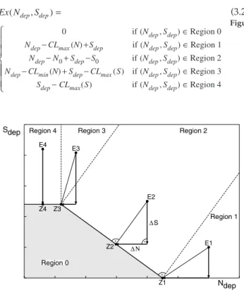
If only one pollutant contributes to an effect, e.g. nitrogen to eutrophication or sulfur to acidification (as assumed before 1994), a unique critical load (CL) can be calculated and compared with deposition (Dep), and the difference has been termed the exceedance of the critical load (Ex = Dep–CL). In the case of two pollutants no unique exceed-ance exists, as is illustrated in Figure 1-2. But for a given deposition of N and S an exceedance has been defined as the sum of the N and S deposition reductions required to achieve non-exceedance by taking the shortest path to the critical load function (see Figure 1-2). Within a grid cell, these exceedances are multiplied by the respective eco-system area and summed to yield the so-called
accumu-lated exceedance(AE) for that grid cell. In addition, the
average accumulated exceedance(AAE) is defined by
divid-ing the AE by the total ecosystem area of the grid cell, and which has thus the dimension of a deposition (see
Chapter 3 for a detailed derivation).
When comparing present or feasible future deposition sce-narios with European critical loads it appeared that non-exceedance could not be reached everywhere. Thus it was decided by integrated assessment modelers to use uniform percentage reductions of the excess deposition (so-called gap closures) to define reduction scenarios. In the following we summarize the different gap closure methods used and illustrate them for the case of a single pollutant.
Figure 1-2. Critical load function for S and acidifying N. It shows that no unique exceedance exists: Let the point E denote the current deposi-tion of N and S. Reducing N
depsubstantially one reaches point Z1 and
thus non-exceedance without reducing S
dep; but non-exceedance can
also be achieved by reducing S
deponly (by a smaller amount) until
reaching Z3. However, an exceedance has been defined as the sum of N
depand Sdepreductions (∆N+∆S) which are needed to reach the critical
load function on the shortest path (point Z2).
In the 1994 Sulphur Protocol, only sulfur was considered as acidifying pollutant (N deposition was fixed; it deter-mined, together with N uptake and immobilization, the sulfur fraction). Furthermore, taking into account the uncertainties in the CL calculations, it was decided to use the 5th percentile of the critical load CDF in a grid cell as the only value representing the ecosystem sensitivity of that cell. And the exceedance was simply the difference between the (current) S deposition and that 5th percentile critical load. This is illustrated in Figure 1-3(a): Critical loads and deposition are plotted along the horizontal axis and the (relative) ecosystem area along the vertical axis. The thick solid and the thick broken lines are two exam-ples of critical load CDFs (which have the same 5th per-centile critical load, indicated by “CL”). “D0” indicates the (present) deposition, which is higher than the CLs for 85% of the ecosystem area. The difference between “D0” and “CL” is the exceedance in that grid cell. It was decid-ed to rdecid-educe the excedecid-edance everywhere by a fixdecid-ed percentage, i.e. to “close the gap” between (present) depo-sition and (5th percentile) critical load. In Figure 1-3(a), a
deposition gap closureof 60% is shown as an example. As
can be seen, a fixed deposition gap closure can result in very different improvements in ecosystem protection percentages (55% vs. 22%), depending on the shape of the critical load CDF. Ndep Sdep CLmin(N) CLmax(N) CLmax(S) Z1 Z3 E Z2 ∆S ∆Ν
Figure 1-3. Cumulative distribution function (CDF; thick solid line) of critical loads and different methods of gap closure: (a) deposition gap closure, (b) ecosystem gap closure, and (c) accumulated exceedance (AE) gap closure. The thick dashed line in (a) and (b) depict another CDF, illustrating how different ecosystem protection follows from the same deposition gap closure (a), or how different deposition reductions are required to achieve the same protection level (b).
In order to take into account all critical loads within a grid cell (and not only the 5th percentile), it was suggested to use an ecosystem area gap closure instead of the deposition gap closure. This is illustrated in Figure 1-2b: for a given deposition “D0” to a grid cell the ecosystem area unprotected, i.e. with deposition exceeding the critical loads, can be read from the vertical axis. After agreeing to a certain (percent) reduction of the unprotected area (e.g. 60%), it is easy to compute for a given CDF the required deposition reduction (“D1” and “D2” in Figure 1-3(b)). Another important reason to use the ecosystem area gap closure is that it can be easily generalized to two (or more) pollutants, which is not the case for a deposition-based exceedance. This generalization became necessary in the preparation for the “multi-pollutant, multi-effect” protocol in the case of acidity critical loads, as both N and S contribute to acidification. Critical load values have been replaced by critical load functions and percentiles replaced by ecosystem protection isolines (see above). However, the use of the area gap closure becomes problematic if only a few critical load values or functions are given for a grid cell. In such a case the CDF becomes highly
discontinuous, and small changes in deposition may result in either no increase in the protected area at all or large jumps in the area protected.
To remedy the problem with the area gap closure caused by discontinuous CDFs, the accumulated exceedance (AE) concept has been introduced (see above and Chapter 3). In the case of one pollutant, the AE is given as the area under the CDF of the critical loads (the entire grey-shaded area in Fig.1-3(c)). Deposition reductions are now negotiated in terms of an AE (or AAE) gap closure, also illustrated in Fig.1-3(c): a 60% AE gap closure is achieved by a deposi-tion “D1” which reduces the total grey area by 60%, resulting in the dark grey area; also the corresponding protection percentage (61%) can be easily derived. The greatest advantage of the AE and AAE is that it varies smoothly as deposition is varied, even for highly discon-tinuous CDFs, thus facilitating optimization calculations in integrated assessment.
The advantages and disadvantages of the three gap clo-sure methods described above are summarized in the fol-lowing table: 100% eq/ha/yr e c o s y s te m a re a CL exceedance
60% deposition gap closure
CL 5% D0 85% 55% 22% D1 (a) 100% eq/ha/yr e c o s y s te m a re a a re a u n p ro te c te d 6 0 % a re a g a p c lo s u re D0 85% D1 D2 (b) 100% eq/ha/yr e c o s y s te m a re a 60% AE gap closure D0 85% D1 61% (c)
1.3 Maps of critical loads/levels and their exceedance
In this section we present European maps of critical loads and levels, as well as their exceedances, which are used in the current protocol negotiations. It should be noted how-ever, that the maps presented here represent only a small fraction of the total critical loads data held at the CCE. The integrated assessment modelers under the LRTAP Convention have been provided a data base containing all the necessary information (such as percentiles and protec-tion isolines) for linking optimizaprotec-tion models to environ-mental effects. The transfer matrices used to calculate the deposition of S and N, and thus exceedances, were provided by the EMEP Meteorological Synthesizing Centre-West (MSC-W) at the Norwegian Meteorological Institute (EMEP 1998). In the following, maps are pre-sented and discussed which illustrate the quantities and concepts summarized in the previous two sections.
Figures 1-4 and 1-5 are maps of the 5th percentiles of the maximum critical load of sulfur, CLmax(S), the minimum critical load of acidifying nitrogen, CLmin(N), the maxi-mum critical load of acidifying nitrogen, CLmax(N), and the critical load of nutrient nitrogen, CLnut(N).They show that maximum critical loads are lowest in the northwest and highest in the southeast. The low values of CLmin(N), as compared to CLnut(N), in the south (Italy, Hungary, Croatia) indicate low values of nitrogen uptake and immobilization, but relatively high values for N leaching and denitrification. The maps on the right display the numbers (in eq ha-1yr-1) underlying the color classes on the left-hand side. The blue grid squares in the right-hand maps indicate data submitted by National Focal Centers (see Chapter 2). Critical loads in the white grids have been computed from the European background data base held at the CCE (see chapter 6 in Posch et al. 1997). The maps in Figures 1-4 and 1-5 also comprise the information on
critical loads provided in printed form to the Working Group on Effects in 1998 (UN/ECE 1998a).
Figure 1-6 shows snapshots of the temporal development (1960–2010) of the exceedance of the 5th percentile maximum critical load of sulfur, CLmax(S), earlier called “critical acid deposition”. The exceedance is calculated due to sulfur deposition alone, implicitly assuming that nitrogen does not contribute to acidification. Although this is probably true at present in many countries as most of the deposited N is still immobilized in the soil or taken up by vegetation, the long-term sustainable maximum deposition for N not to contribute to acidification is given by CLmin(N). However, the main purpose of Figure 1-6 is to illustrate the change in the acidity critical load exceed-ance over time. As can be seen from the maps, the size of area and magnitude of exceedance peaked around 1980, with a decline afterwards to a situation in 1995 which is better than in 1960. Further improvements can be expected when the Current emission Reduction Plans (the so-called CRP scenario, UN/ECE 1998b) is implemented, which includes all reduction measures already legislated by member countries (inter alia the 1994 Sulphur Protocol). However, further emission reductions are needed to reach the goal that deposition of S and N does not exceed criti-cal loads of acidity over all of Europe.
As mentioned in the previous section, a unique exceedance does not exist when considering both sulfur and nitrogen, but for a given deposition of S and N one can always determine whether there is non-exceedance or not. The two maps at the top of Figure 1-7 show the percent of ecosystem area protected from acidifying deposition of S and N in 1990 and 2010. In 1990 less than 10% of the ecosystem area is protected in large parts of central and western Europe as well as on the Kola peninsula. Under the CRP scenario, the situation improves almost every-where, but still far from reaching complete protection.
Advantages Disadvantages
Deposition gap closure • Easy to use even for discontinuous • Takes only one CL value (e.g. 5th (used for the 1994 UN/ECE CDFs (e.g. grid cells with only percentile) into account.
Sulphur Protocol) one CL). • May result in no increase of protected
area.
• Difficult to define for two pollutants.
Ecosystem area gap closure • In line with the goals of CL use • Difficult (or even impossible) to define (used for the EU Acidification (maximum ecosystem protection). a gap closure for discontinuous CDFs Strategy) • Easy to apply to any number of (e.g. grid cells with only one CL).
pollutants.
Accumulated Exceedance (AE) • AE (and AAE) is a smooth and convex • AE stretches the limits of the critical
gap closure function of deposition even for load definition.*
(used for the UN/ECE multi- discontinuous CDFs. • Exceedance definition not unique
pollutant, multi-effects protocol) for 2 or more pollutants.
Figure 1-4. The 5th percentiles of the maximum critical loads of sulfur, CLmax(S), and of the minimum critical loads of acidifying nitrogen, CLmin(N).
The maps on the right display the numbers (in eq ha-1yr-1) underlying the color classes on the left-hand side. The blue grid squares in the right-hand
maps indicate data from National Focal Centers. eq/ha/yr < 200 200 – 400 400 – 700 700 – 1000 1000 – 1500 > 1500 12 13 14 15 16 17 18 19 20 21 22 23 24 25 26 27 28 29 30 31 32 33 34 35 36 37 38 1 3 5 7 9 11 13 15 17 19 21 23 25 27 29 31 33 35 37 CLmax(S) (5th percentile) CCE/RIVM eq/ha/yr (**** CL>9999) national CL data 996 2614 3824 4146 1084 1002 2578 2158 3777 3735 1479 1288 3246 3008 3247 3859 **** 2709 2239 2259 2733 3564 ******** 711 1962 2455 3384 2960 ************ 1965 926 1690 2557 2800 3583 **** ******** 569 **** 3127 1524 **** 4758 ******** 450 450 1154 1154 2864 2488 2053 1670 512 512 1424 1424 2218 2055 1762 1320 1005 1005 1670 954 954 954 1324 1154 1670 3089 2447 1351 1072 509 1670 1120 1005 770 770 954 954 1106 771 1154 930 979 977 1842 1827 1110 644 479 419 435 1005 1005 770 970 1324 873 649 777 1604 2177 1775 1978 1805 1205 1966 805 649 519 469 700 696 1320 1170 970 724 737 470 771 2247 1894 1779 1921 1849 2021 624 583 600 578 585 353 1670 955 838 410 490 626 590 1132 7157 7184 7676 6234 5978 9055 550 340 321 326 583 335 1031 683 533 655 677 570 933 1302 1798 7651 6675 6843 6751 5491 7193 7010 6551 7323 9188 529 330 250 839 704 296 485 881 608 351 752 764 1069 1069 5154 4745 4806 2236 6418 6149 7319 519 239 219 413 137 267 628 668 633 656 567 835 1069 5823 6625 6478 2236 2101 7446 7711 529 1317 351 332 433 587 947 669 29624 1335 2797 6790 5371 4590 3649 5571 319 163 1760 1220 793 256 784 716 659 1089 1501 25535 1674 2063 3746 4601 2497 8986 610 220 124 304 390 375 913 940 523 697 959 1300 827 1830 1663 1602 1692 4694 4022 199 154 174 295 335 238 318 737 831 544 742 1239 1883 1897 831 316 1536 3215 289 210 294 244 205 219 2194 3273 2076 786 647 294 895 1918 837 997 148 1415 291 31692141 260 406 2505 2109 2312 368 294 311 659 1740 2561 2865 3014 2975 2323 126 228 154 187 383 260 2190 3333 2246 869 408 405 748 748 2282 2545 2955 2652 2490 261 213 201 106 365 278 921 1580 1139 456 410 406 748 1205 2181 2499 2127 1776 373 168 147 229 295 360 311 284 882 1079 1140 772 946 1071 1420 1634 2256 2001 1924 983 1756 1779 435 93 75243 230 474 331 378 726 924 1087 1133 1126 1087 1113 1364 1434 1957 864 1385 1194 1752 1785 432 93112 272 206 343 308 585 585 885 952 1028 1183 1138 1347 1347 2014 1717 1096 1590 982 992 1897 358 286 191 159 177 260 339 379 402 603 634 717 1176 1286 1270 962 981 1283 1048 995 993 999 1983 1253 99 211 263 225 198 232 334 351 391 555 597 606 947 1867 2368 917 986 1206 1042 1130 992 993 999 2004 1763 116 259 242 236 228 323 328 358 524 551 588 596 729 839 831 1012 1208 1185 1448 1450 1611 1742 1743 1767 247 228 245 292 317 325 479 525 557 564 586 683 780 1032 997 1443 1439 1610 230 258 305 310 331 447 513 541 553 559 891 779 1023 1212 231 241 306 316 325 447 501 520 548 568 874 924 1003 1227 226 236 239 317 318 451 482 517 534 584 868 811 963 918 233 233 235 318 319 459 489 506 532 689 684 694 871 789 268 232 232 328 321 322 488 533 534 665 684 882 869 1302 12 13 14 15 16 17 18 19 20 21 22 23 24 25 26 27 28 29 30 31 32 33 34 35 36 37 38 1 3 5 7 9 11 13 15 17 19 21 23 25 27 29 31 33 35 37 CLmax(S) (5th percentile) CCE/RIVM eq/ha/yr < 200 200 – 400 400 – 700 700 – 1000 1000 – 1500 > 1500 12 13 14 15 16 17 18 19 20 21 22 23 24 25 26 27 28 29 30 31 32 33 34 35 36 37 38 1 3 5 7 9 11 13 15 17 19 21 23 25 27 29 31 33 35 37 CLmin(N) (5th percentile) CCE/RIVM eq/ha/yr national CL data 266 322 282 251 426 266 251 251 251 266 426 266 251 251 252 272 273 369 426 255 252 252 251 272 826 414 256 253 256 255 265 272 826 586 483 266 255 255 257 255 326 602 299 266 260 252 308 255 255 340 266 266 266 193 207 161 370 340 340 390 390 193 196 182 341 341 370 370 370 390 341 370 266 196 168 179 216 216 141 370 341 341 341 341 370 266 161 496 266 391 454 454 161 439 216 216 141 141 141 341 341 341 266 390 168 154 786 443 168 286 168 154 154 496 216 216 141 141 141 141 341 341 266 471 329 157 161 475 786 300 168 786 182 216 141 141 141 141 141 370 266 356 298 445 139 154 161 180 351 351 351 370 351 141 141 141 141 141 141 340 340 464 428 428 428 342 428 357 129 129 231 174 174 351 351 351 351 351 141 141 141 141 321 340 499 428 392 428 410 535 0 0 129 180 163 598 351 351 351 284 275 141 464 392 392 392 428 520 499 308 0 0 405 165 476 420 583 351 351 141 244 464 392 392 337 386 449 342 0 0 701 193 629 550 376 359 141 27284 354 244 392 371 361 363 332 356 235 0 643 367 362 558 312 456 33 29 27 30163 273 107 371 352 356 366 371 293 349 321 342 427 454 504 26 30 30 33124 166 277 360 387 376 366 376 417 391 1054 948 2730 796 30 33 33 4614696243 334 553 361 255 124 249 191 1351 1398 3021 796 32 0 5 60 51 20 0 334 334 473 472 123 123 191 266 330 577 626 740 31 0 12 9313941260 260 334 472 472 123 409 409 260 391 336 677 704 0 0 45 27124 100 160 35090214 471 472 489 249 277 391 391 433 33 0 2 28 56 74103 12222 90 91 9910099485 84391 391 271 445 432 70 29 0 6 39 72 76 86 23 25 90 98101 95184 482 486 82391 172 171 430 149 172 33 0 7 46 51 57 68 19 55 89104 97442 591 82 80 69 71166 166 174 152 151 33 33 40 40 44 98207 15921 23 86143 9478 82 82 71172 175 162 156 151 153 780 33 29 33 80330 207 208 38027 19 56151 149 180 58564167 427 425 147 376 148 148 151 158 33154 118 119 20742241 18 20 56150 18588380 612 431 430 428 156 149 142 141 146 152 232 24678 42 42 43 19 61144 203 18386174 663 696 421 421 152 23 22 42 42 84 56 56 58317 147 147 142 432 698 15323 42 42 79 18 17 18142 138 143 139 701 697 23 22 42 42 42184 17 21 7477233 370 427 426 21 22 23 23 23184 19 5423373310 236 242 423 22 22 22 23 22 79 55 54 5672236 231 72 69 12 13 14 15 16 17 18 19 20 21 22 23 24 25 26 27 28 29 30 31 32 33 34 35 36 37 38 1 3 5 7 9 11 13 15 17 19 21 23 25 27 29 31 33 35 37 CLmin(N) (5th percentile) CCE/RIVM
Figure 1-5. The 5th percentiles of the maximum critical loads of acidifying nitrogen, CLmax(N), and of the critical loads of nutrient nitrogen, CLnut(N).
The maps on the right display the numbers (in eq ha-1yr-1) underlying the color classes on the left-hand side. The blue grid squares in the right-hand
maps indicate data from National Focal Centers. eq/ha/yr < 200 200 – 400 400 – 700 700 – 1000 1000 – 1500 > 1500 12 13 14 15 16 17 18 19 20 21 22 23 24 25 26 27 28 29 30 31 32 33 34 35 36 37 38 1 3 5 7 9 11 13 15 17 19 21 23 25 27 29 31 33 35 37 CLmax(N) (5th percentile) CCE/RIVM eq/ha/yr (**** CL>9999) national CL data 1372 3475 4571 4866 1630 1430 3435 3083 4498 4511 2069 1812 3987 3682 4072 4562 **** 9733 8131 3057 3492 4377 ******** 3010 2938 3326 4046 3662 ************ 3010 2510 2967 3378 3609 4276 **** ******** 3464 **** 4138 2054 **** 5604 ******** 852 852 1421 1421 3375 3803 6333 2040 852 852 1954 1954 2786 2751 2699 1661 1623 1623 2040 1371 1371 1371 1854 1421 2040 9445 3187 1573 1290 794 2040 1461 1511 1111 1111 1371 1371 1854 1691 1421 1326 1432 1430 2282 2528 1431 1157 764 704 758 1623 1623 1111 1271 1854 1721 1720 3496 3111 3178 3492 3468 3151 3237 2462 1276 1120 791 754 1120 1096 1661 1511 1271 1254 1642 684 2226 3364 7416 5809 2652 7237 3107 996 899 791 852 934 656 2040 1271 1497 762 1279 1408 1795 4182 ******** **************** 834 624 654 670 724 619 1955 1502 1413 1512 1398 1418 1861 2441 2214 8664 7615 **** 9116 6529 **** ******** ******** 814 641 575 981 1722 1024 1347 1727 1282 1087 1644 2025 1069 1069 6132 5815 5882 2834 **** ******** 791 574 694 1060 652 860 1258 1417 1238 1460 1112 835 1069 **** 6790 6954 2773 2698 ******** 814 1572 1327 983 1071 1091 1941 1589 967 789 1779 3904 6983 6000 5202 4155 **** 604 249 2051 1711 1496 1328 1720 1915 1908 2680 2683 717 1069 2656 3088 **** 5167 2839 9442 870 304 194 481 559 880 1227 2328 1616 1910 2392 3062 1581 2664 2504 2576 2676 5148 4531 278 233 317 474 572 641 788 1892 2125 1742 2028 2846 4110 3366 2002 2091 5587 **** 471 318 622 498 534 496 2787 3970 2730 1785 1174 917 3417 3686 2188 2573 5375 7872 477 473 167 448 564 632 3134 2717 3866 1556 1337 1221 1212 2380 9158 ************ 8483 198 337 448 576 795 555 4808 4141 2872 1898 1363 1329 1440 1530 2927 9128 **** 9543 9003 352 331 428 405 723 601 1311 4130 1315 1463 1381 1361 1797 4216 7828 8978 7751 2209 527 186 188 433 597 794 674 592 1074 1277 1473 1279 1447 1446 1906 1720 8147 7318 7116 2039 2212 1859 632 102 129 451 926 837 715 849 856 1173 1267 1319 1263 1354 1756 1641 1910 7228 1133 1802 2038 1969 1962 617 129 199 623 498 774 659 720 845 1131 1170 1315 1826 1774 1429 1448 2186 1881 1756 1759 1385 1604 2054 557 584 561 361 542 528 560 704 741 761 870 1117 1415 1364 1351 1346 1370 1663 1758 1379 1370 1376 2135 2032 175 441 526 382 549 517 544 758 735 708 726 928 1413 2285 3284 1299 1370 1883 1849 1413 1370 1373 1776 2156 1926 204 456 416 422 463 417 675 651 674 681 855 858 932 1226 1664 1725 1897 1848 1736 1759 1760 1884 1893 1922 508 523 441 392 401 426 651 679 817 852 1200 810 1005 1741 1705 1869 1862 1762 406 342 388 400 419 584 661 676 871 877 1048 1006 1734 1910 405 336 404 406 426 629 655 675 865 795 1043 1213 1715 1924 295 295 334 412 417 650 666 678 704 963 1142 1184 1672 1637 290 331 333 416 449 652 646 621 996 975 1000 1009 1384 1627 289 330 330 449 417 509 648 621 653 951 995 1119 1107 1376 12 13 14 15 16 17 18 19 20 21 22 23 24 25 26 27 28 29 30 31 32 33 34 35 36 37 38 1 3 5 7 9 11 13 15 17 19 21 23 25 27 29 31 33 35 37 CLmax(N) (5th percentile) CCE/RIVM eq/ha/yr < 200 200 – 400 400 – 700 700 – 1000 1000 – 1500 > 1500 12 13 14 15 16 17 18 19 20 21 22 23 24 25 26 27 28 29 30 31 32 33 34 35 36 37 38 1 3 5 7 9 11 13 15 17 19 21 23 25 27 29 31 33 35 37 CLnut(N) (5th percentile) CCE/RIVM eq/ha/yr national CL data 269 332 332 322 446 283 267 284 295 282 456 277 269 267 270 279 275 553 728 284 270 270 284 279 959 536 322 275 271 310 303 313 959 669 553 382 316 271 289 281 415 853 504 376 336 306 326 302 344 370 366 366 366 407 421 389 375 370 341 390 390 390 407 411 396 389 379 341 341 370 370 370 390 370 370 366 370 382 382 379 933 644 850 370 341 370 370 370 370 366 286 536 366 370 489 489 375 529 933 644 933 850 850 341 341 391 366 390 346 354 1021 479 475 314 382 368 393 532 455 574 644 850 850 850 341 391 366 471 571 354 279 596 1034 314 382 484 396 714 714 714 714 850 850 370 366 471 398 645 318 286 339 427 500 661 541 405 450 423 714 714 714 714 850 714 451 451 563 446 455 593 499 710 630 262 223 567 356 345 438 410 358 481 458 714 714 714 851 433 451 554 455 420 483 593 710 286 1600 240 248 241 602 364 359 385 714 714 714 502 420 420 438 455 530 538 321 399 1200 489 170 484 432 594 470 524 714 476 502 411 411 383 425 531 401 358 167 711 208 639 569 382 451 714 393 482 573 809 420 411 398 397 393 457 38777663 399 364 566 321 469 500 393 393 393 433 393 240 448 394 387 406 430 414 413 376 410 432 462 509 393 393 393 393 293 379 291 410 437 414 401 413 450 413 1118 1016 2868 803 393 393 393 270 292 288 243 385 786 394 333 236 270 209 1412 1498 3076 803 393 393 307 374 256 380 1165 398 379 539 535 204 205 220 278 335 585 633 762 393 180 230 364 238 161 350 460 396 536 546 203 521 526 266 396 341 684 711 191 149 206 248 206 210 234 350 230 379 546 546 624 263 282 396 396 524 434 393 220 217 199 211 200 226 164 232 356 403 340 279 609 334 396 397 281 561 547 180 393 185 147 222 200 206 195 154 181 232 249 350 294 336 596 610 400 397 301 295 520 240 306 393 129 141 188 218 217 205 150 183 227 333 347 761 816 328 321 379 278 272 273 305 249 201 393 158 159 189 204 293 297 282 145 149 218 340 377 313 328 338 374 292 298 244 255 198 201 829 393 161 150 148 397 295 326 439 162 139 180 303 301 473 889 355 360 509 476 199 408 187 189 196 207 261 146 177 338 156 353 136 140 184 301 334 290 500 877 615 602 483 214 184 171 166 182 188 259 281 181 154 153 157 138 207 284 329 478 156 267 1007 865 463 451 190 240 109 152 153 260 180 181 195 490 275 276 263 768 958 268 111 151 152 169 134 132 135 273 208 265 261 958 947 114 111 153 151 153 361 132 144 206 238 540 659 555 552 109 110 112 112 113 361 137 174 353 269 465 477 417 478 109 111 110 111 111 170 177 171 183 194 362 439 171 163 12 13 14 15 16 17 18 19 20 21 22 23 24 25 26 27 28 29 30 31 32 33 34 35 36 37 38 1 3 5 7 9 11 13 15 17 19 21 23 25 27 29 31 33 35 37 CLnut(N) (5th percentile) CCE/RIVM
Figure 1-6. Temporal development (1960–2010) of the exceedance of the 5th percentile maximum critical load of sulfur (“acidity critical load”). White areas indicate non-exceedance or lack of data (e.g. Turkey). Sulfur deposition data were provided by the EMEP/MSC-W (EMEP 1998).
eq/ha/yr < 200 200 – 400 400 – 700 700 – 1000 1000 – 1500 > 1500 Exceedance of 5% CLmax(S) 1960 Dep-data: EMEP/MSC-W CL-data: CCE/RIVM eq/ha/yr < 200 200 – 400 400 – 700 700 – 1000 1000 – 1500 > 1500 1970 Dep-data: EMEP/MSC-W CL-data: CCE/RIVM eq/ha/yr < 200 200 – 400 400 – 700 700 – 1000 1000 – 1500 > 1500 1975 Dep-data: EMEP/MSC-W CL-data: CCE/RIVM eq/ha/yr < 200 200 – 400 400 – 700 700 – 1000 1000 – 1500 > 1500 1980 Dep-data: EMEP/MSC-W CL-data: CCE/RIVM eq/ha/yr < 200 200 – 400 400 – 700 700 – 1000 1000 – 1500 > 1500 1985 Dep-data: EMEP/MSC-W CL-data: CCE/RIVM eq/ha/yr < 200 200 – 400 400 – 700 700 – 1000 1000 – 1500 > 1500 1990 Dep-data: EMEP/MSC-W CL-data: CCE/RIVM eq/ha/yr < 200 200 – 400 400 – 700 700 – 1000 1000 – 1500 > 1500 1995
Dep-data: EMEP/MSC-WCL-data: CCE/RIVM
eq/ha/yr < 200 200 – 400 400 – 700 700 – 1000 1000 – 1500 > 1500 CRP 2010
Figure 1-7. Top: The percentage of ecosystem area protected (i.e. non-exceedance of critical loads) from acidifying deposition of sulfur and nitrogen in 1990 (left) and in the year 2010 according to current emission reduction plans (right). Bottom: The accumulated average exceedance (AAE) of the acidity critical loads by sulfur and nitrogen deposition in 1990 (left) and 2010 (right). Sulfur and nitrogen deposition data were provided by the EMEP/MSC-W (EMEP 1998). %protected < 10 10 – 20 20 – 30 30 – 50 50 – 70 70 – 99 100 12 13 14 15 16 17 18 19 20 21 22 23 24 25 26 27 28 29 30 31 32 33 34 35 36 37 38 1 3 5 7 9 11 13 15 17 19 21 23 25 27 29 31 33 35 37
Ecosystem protection percentage 1990
Dep-data: EMEP/MSC-WCL-data: CCE/RIVM
%protected < 10 10 – 20 20 – 30 30 – 50 50 – 70 70 – 99 100 12 13 14 15 16 17 18 19 20 21 22 23 24 25 26 27 28 29 30 31 32 33 34 35 36 37 38 1 3 5 7 9 11 13 15 17 19 21 23 25 27 29 31 33 35 37
Ecosystem protection percentage CRP 2010
Dep-data: EMEP/MSC-WCL-data: CCE/RIVM
eq/ha/yr no exceedance < 200 200 – 400 400 – 700 700 – 1000 1000 – 1500 > 1500 12 13 14 15 16 17 18 19 20 21 22 23 24 25 26 27 28 29 30 31 32 33 34 35 36 37 38 1 3 5 7 9 11 13 15 17 19 21 23 25 27 29 31 33 35 37
Accumulated Average Exceedance 1990
Dep-data: EMEP/MSC-WCL-data: CCE/RIVM
eq/ha/yr no exceedance < 200 200 – 400 400 – 700 700 – 1000 1000 – 1500 > 1500 12 13 14 15 16 17 18 19 20 21 22 23 24 25 26 27 28 29 30 31 32 33 34 35 36 37 38 1 3 5 7 9 11 13 15 17 19 21 23 25 27 29 31 33 35 37
Accumulated Average Exceedance CRP 2010
To be able to compare deposition of S and N with the acidity critical load function, an exceedance quantity has been defined (see previous sections). This average accumulated exceedance (AAE) is the amount of excess acidity averaged over the total ecosystem area in a grid square. The two maps at the bottom of Figure 1-7 show the AAE for 1990 and 2010 (CRP scenario). In 1990 the highest excess acidity occurs in central Europe, the pattern roughly matching with the ecosystem protection percent-ages for the same year. Under the CRP scenario in 2010, excess acidity is reduced nearly everywhere, with a peak remaining in the “Black Triangle” of Germany, Poland and the Czech Republic.
Nitrogen not only contributes to acidification and eutro-phication, but is also a precursor for the formation of tropospheric ozone. High levels of ground-level ozone concentration have adverse effects on forests and cause yield reductions in crops. Therefore, critical levels for forests and crops have been derived (Kärenlampi and Skärby 1996). They are based on the “AOT” concept, i.e. the accumulated exposure over a threshold of 40 ppb (called AOT40) during daylight hours in the growing season (May-July for crops and semi-natural vegetation).
The critical level for crops is 3000 ppb·hours (shaded blue in Figure 1-8) independent of the location (so-called Level I critical level). In Figure 1-8 the AOT40 for crops is shown for eight different years between 1985 and 1996. The modeled 6-hourly ozone concentrations have been provided by the EMEP/MSC-W (Simpson et al. 1997). The eight maps illustrate that ozone concentrations vary strongly from year to year, and thus a five-year average is recommended for integrated assessment purposes (UBA 1996). The size of the grid squares in Figure 1-8 corre-sponds to the percentage of arable land in that
150×150km2EMEP grid cell, thus indicating the potential stock-at-risk. However, more work is needed to refine both the land use data and the critical levels (site-dependent Level II critical levels) before an economic evaluation of ozone impacts can be attempted in earnest.
References
Downing, R.J., J.-P. Hettelingh and P.A.M. de Smet (eds.), 1993. Calculation and Mapping of Critical Loads in Europe: CCE Status Report 1993. National Institute of Public Health and the Environment (RIVM) Rep. 259101003, Bilthoven, Netherlands. EMEP, 1998. Transboundary acidifying air pollution in Europe, MSC-W
Status Report 1998 - Parts 1 and 2. EMEP/MSC-W Report 1/98, Norwegian Meteorological Institute, Oslo, Norway.
Hettelingh, J.-P., Downing, R.J. and P.A.M. de Smet (eds.), 1991. Calculation and Mapping of Critical Loads in Europe: CCE Technical Report No. 1. National Institute of Public Health and the Environment (RIVM) Rep. 259101001, Bilthoven, Netherlands. Hettelingh, J.-P., M. Posch, P.A.M. de Smet and R.J. Downing, 1995.
The use of critical loads in emission reduction agreements in Europe. Water Air Soil Pollut. 85:2381-2388.
Kärenlampi, L. and L. Skärby (eds.), 1996. Critical Levels for Ozone in Europe: Testing and Finalizing the Concepts. UN-ECE Workshop Report. Univ. of Kuopio, Dept. of Ecology and Environmental Science.
Nilsson, J. and P. Grennfelt (eds.), 1988. Critical Loads for Sulphur and Nitrogen. Nord 1988:97, Nordic Council of Ministers, Copenhagen, Denmark, 418 pp.
Posch, M., P.A.M. de Smet, J.-P. Hettelingh, and R.J. Downing (eds.), 1995. Calculation and Mapping of Critical Thresholds in Europe: CCE Status Report 1995. National Institute of Public Health and the Environment (RIVM) Rep. 259101004, Bilthoven, Netherlands. Posch, M., J.-P. Hettelingh, P.A.M. de Smet and R.J. Downing (eds.),
1997. Calculation and Mapping of Critical Thresholds in Europe: CCE Status Report 1997. National Institute of Public Health and the Environment (RIVM) Rep. 259101007, Bilthoven, Netherlands. Simpson, D., K. Olendrzynski, A. Semb, E. Støren and S. Unger, 1997.
Photochemical oxidant modelling in Europe: Multi-annual model-ling and source-receptor relationships. EMEP/MSC-W Report 3/97. Norwegian Meteorological Institute, Oslo, Norway. UBA, 1996. Manual on Methodologies and Criteria for Mapping
Critical Levels/Loads and geographical areas where they are exceeded. UN/ECE Convention on Long-range Transboundary Air Pollution. Federal Environmental Agency (Umweltbundesamt), Texte 71/96, Berlin.
UN/ECE, 1998a. Updated maps of critical loads, uncertainties and exceedance. Document EB.AIR/WG.1/1998/5, Geneva, 8 pp. UN/ECE, 1998b. Integrated assessment modelling. Document
Figure 1-8. The accumulated exposure to ground-level ozone concentrations over a threshold of 40 ppb (AOT40 for crops) in eight years between 1985 and 1996. The blue-shaded grids indicate areas where the critical AOT40 level of 3000 ppb·hours is not exceeded. The size of a grid square
corre-sponds to the percentage of arable land in that 150×150km2EMEP grid cell. Ozone concentration data were provided by the EMEP/MSC-W
(Simpson et al. 1997). ppm-h < 3 3 – 6 6 – 9 9 –12 >12
AOT40c over arable land 1985
O3-data: EMEP/MSC-W LU-data: CCE/RIVM ppm-h < 3 3 – 6 6 – 9 9 –12 >12 1989 O3-data: EMEP/MSC-W LU-data: CCE/RIVM ppm-h < 3 3 – 6 6 – 9 9 –12 >12 1990 O3-data: EMEP/MSC-W LU-data: CCE/RIVM ppm-h < 3 3 – 6 6 – 9 9 –12 >12 1992 O3-data: EMEP/MSC-W LU-data: CCE/RIVM ppm-h < 3 3 – 6 6 – 9 9 –12 >12 1993
O3-data: EMEP/MSC-WLU-data: CCE/RIVM
ppm-h < 3 3 – 6 6 – 9 9 –12 >12 1994
O3-data: EMEP/MSC-WLU-data: CCE/RIVM
ppm-h < 3 3 – 6 6 – 9 9 –12 >12 1995
O3-data: EMEP/MSC-WLU-data: CCE/RIVM
ppm-h < 3 3 – 6 6 – 9 9 –12 >12 1996
2. Summary of National Data
P.A.M. de Smet and M. Posch
Introduction
At the request of the UN/ECE Working Group of Effects (WGE), the Coordination Center for Effects (CCE) periodically asks countries to submit up-to-date national critical loads data, so that the integrated assessment modeling groups participating in LRTAP Convention activities can work with the latest data. Such a request gives National Focal Centers (NFCs) the opportunity to submit their latest results. This chapter describes briefly the process and summarizes the results of the 1998 data update cycle. It lists the countries that contributed national data and provides an overview of the ecosystems selected as receptors and density (resolution) of the national data. The cumulative distributions of the critical loads are compared and the input parameters needed to compute the critical loads for forest soils are analyzed in detail.
2.1 Overview of national contributions
The following timetable illustrates the 1998 update of national critical load data:
29.9.1997 CCE issues a call for updated data to all NFCs, as requested by the Working Group on Effects (WGE), with a deadline for
submission of 15 January 1998.
14.3.1998 Preliminary European critical load data sets are made available to Task Force on Integrated Assessment Modelling (TFIAM). 9.4.1998 CCE sends the updated data base to NFCs for
verification and comments.
23.4.1998 CCE provides the updated data sets to the Task Force on Mapping (TFM).
11.5.1998 New data and maps are presented at CCE workshop in Kristiansand, Norway. 15.5.1998 TFM adopts the new data set, with the
understanding that 5 countries will submit minor modifications before 15 June 1998. 7.7.1998 CCE provides TFIAM, NFCs and WGE with
final data sets.
26.8.1998 WGE adopts data sets and maps as final version for update round of the year 1998. 4.9.1998 Working Group on Strategies (WGS)
announces a “data freeze” for all input data used in the preparations and negotiations of the “multi-pollutant, multi-effect” protocol.
The number of countries that submitted data in 1998 has increased to 24 (listed in Table 2-1). These national contributions have been adopted by the WGE in August 1998. Countries that contributed revised data are Austria, Belgium, Finland, France, Germany, Ireland, Italy, Poland, Russian Federation, Sweden and the United Kingdom. Four countries contributed national data for the first time: Belarus, Bulgaria, Republic of Moldova and Slovakia. The revision of Belgian data included a first-time contribution for the Wallonian part of the country, while the Flemish data remained unchanged from 1997. The revision of the Russian data consisted in a simple area correction of its 1996 data. No changes were submitted for the Netherlands and Spain (which continue to use 1996 data) or for Croatia, Czech Republic, Denmark, Estonia, Hungary, Norway and Switzerland (which submitted data in 1997). Most of the European mapping domain is now covered by national contributions. Further details on most countries’ activities can be found in Part III of this report, as well as the CCE Status Report 1997.
At previous mapping workshops, the CCE and NFCs have agreed to the following rules concerning the application of critical loads data for areas that are not covered by national contributions:
(i) For all grid cells that do not cover a country that con-tributes national data, critical loads are computed using the European background data base held at the CCE. (See Posch et al. 1997, Chapter 6 for a descrip-tion of this data base).
(ii) For grid cells that cover parts of one or more countries which have submitted national data, calculations are based on the national critical loads data for this cell only, no matter how small the area or how few data are supplied. For these grid cells, no background data are included.
2.2 Scope of national contributions
National Focal Centers have selected a variety of eco-system types as receptors for calculating and mapping critical loads. For most ecosystem types (e.g. forests), critical loads are calculated for both acidity and eutrophi-cation. Other receptor types (e.g. streams and lakes) have only critical loads for acidity, on the assumption that eutrophication does not occur in these ecosystems. For some receptors, like most semi-natural vegetation, only critical loads for nutrient nitrogen are computed.
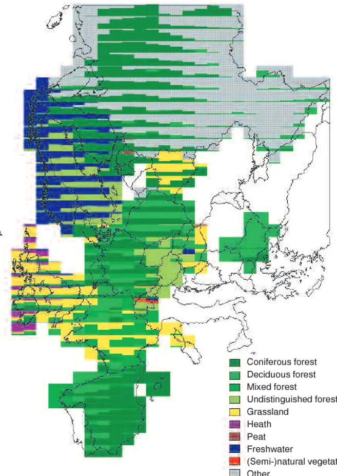
Table 2-2 shows by country the ecosystem types, number of records, their total (summed) area in km2and their percentage of the country area. Figure 2-1 shows the distribution of ecosystem types for which critical loads have been calculated, and their areas as a percentage of total country area. The diversity of ecosystem types selected by the countries as being sensitive to acidification and/or eutrophication has been reduced into a more limited set of types for presentation reasons. The histogram in Figure 2-1 shows that most countries have concentrated on mapping critical loads for forest soils, while some countries (e.g. Finland, Norway and Sweden) have also mapped surface waters as an important receptor. Norway and Switzerland have significant areas of (semi-)natural vegetation selected as a receptor. Ireland and the United Kingdom have considerable areas with critical loads for heathland, while grasslands represent substantial areas in Austria, Belarus, France, Italy, the Republic of Moldova, and the United Kingdom.
Table 2-3 provides details on the number, area coverage, and the density of ecosystems for which NFCs have
submitted critical loads of acidity and/or nutrient nitrogen. National data provided for acidity critical loads are summarized in columns A through D. Column A gives the number of ecosystems for which acidity critical loads (CLmax(S), CLmin(N), and CLmax(N)) have been calculated. Columns B and C show the total area of these ecosystems and the percentage of the country covered by these eco-systems, respectively. The average size of an ecosystem is given in Column D (D=B/A). Similar information for
CLnut(N)is provided in Columns E through H. Columns I through L provide information on ecosystems for which
bothacidity and nutrient critical loads have been
submitted. Columns M through P provide information for those ecosystems for which critical loads of acidity and/or nutrient nitrogen have been calculated (col. M=A+E–I). The wide range in the number and density of ecosystems among countries can be seen from the table. For most countries, critical loads of acidity and nutrient nitrogen are computed on the same set of ecosystems; thus the number and area of ecosystems are the same for both types of critical loads.
Table 2-1. National data version used at present (1999) and most recent year of adoption by the WGE.
Year of adoption by the WGE
Country Code 1996 1997 1998 Remark
Austria AT ✓ Update of earlier contribution.
Belgium BE ✓ (✓) First contribution for Wallonian part of country.
Belarus BY ✓ First national contribution.
Bulgaria BG ✓ First national contribution.
Croatia HR ✓ Only EMEP 50×50 km2grid cells (79,43) and (80,43).
Czech Republic CZ ✓
Denmark DK ✓
Estonia EE ✓
Finland FI ✓ Update of earlier contribution.
France FR ✓ Update of earlier contribution.
Germany DE ✓ Update of earlier contribution.
Hungary HU ✓
Ireland IE ✓ Update of earlier contribution.
Italy IT ✓ Update of earlier contribution.
Netherlands NL ✓
Norway NO ✓
Poland PL ✓ Update of earlier contribution.
Republic of Moldova MD ✓ First national contribution.
Russian Federation RU ✓ (✓) Correction of area from 1996 version only.
Slovakia SK ✓ First national contribution.
Spain ES ✓
Sweden SE ✓ Update of earlier contribution.
Switzerland CH ✓
United Kingdom UK ✓ Update of earlier contribution.
Table 2-2. Type and number of ecosystems for which critical loads data are provided by National Focal Centers.
No. of Area
CCE eco- % of
Country Ecosystem type code systems km2 country Remarks
Austria Forest f 6,604 49,918 59.54
Oligotrophic bog p 205 1,536 1.83 Only CLnut(N).
Alpine grassland g 1,092 8,236 9.82 Only CLnut(N).
Belgium Coniferous forest c 835 2,642 8.66 Flanders: 652 ecosystems,
Deciduous forest d 1,201 4,154 13.61 including 75 mixed forests.
Mixed forest m 490 225 0.74 Wallonia: 1880 ecosystems,
Lake w 6 3 0.01 including 415 mixed forests.
Belarus Coniferous forest c 234 19,398 9.34
Deciduous forest d 79 1,258 0.61
Grassland g 242 29,630 14.27
Bulgaria Coniferous forest c 29 7,579 6.83
Deciduous forest d 55 41,897 37.75
Croatia Coniferous forest c 18 1,438 2.54 Two EMEP 50×50 km2grid cells.
Deciduous forest d 16 1,261 2.23
Czech Forest f 29,418 26,568 33.69
Republic
Denmark Coniferous forest c 6,496 2,336 5.42 Spruce and pine species.
Deciduous forest d 3,261 813 1.89 Beech and oak species.
Grass g 9,027 747 1.73 Only acidity CLs.
Estonia Coniferous forest c 99 13,380 29.58 Spruce and pine species.
Deciduous forest d 26 3,200 7.08
Bog p 15 2,330 5.15
Finland Coniferous forest c 2,049 148,941 44.05 Spruce and pine species.
Deciduous forest d 1034 16,104 4.76
Lake w 1450 107,816 31.88 Only acidity CLs.
France Coniferous forest c 28 20,856 3.83 The original data base with
Deciduous forest d 83 75,432 13.87 detailed ecosystem types
Mixed forest m 302 131,757 24.22 has been reclassified into
Grassland (agricultural) g 178 89,658 16.48 these 4 groups.
Germany Coniferous forest c 227,506 56,877 15.93
Deciduous forest d 91,957 22,989 6.44
Mixed forest m 90,892 22,723 6.36
Hungary Unspecified forest f 7 1,022 1.10
Coniferous forest c 5 43 0.05 Deciduous forest d 8 557 0.60 Grassland/reed/marsh g 12 889 0.96 Heath h 4 13 0.01 Bog p 4 52 0.06 Lake w 2 271 0.29
Ireland Coniferous forest c 10,078 2,445 3.48
Deciduous forest d 8,951 1,808 2.57
Natural grassland g 7,539 2,044 2.91
Moors and heathland h 7,304 2,605 3.71
Fresh waters w 175 175 0.25
Italy Coniferous forest c 63 17,225 5.72 10 with only CLnut(N).
Deciduous forest d 165 60,577 20.11 56 with only CLnut(N). Mediterranean forest m 110 14,109 4.68 35 with only CLnut(N).
Tundra h 46 4,709 1.56
Acid grassland g 118 23,235 7.71 25 with only CLnut(N).
Netherlands Coniferous forest c 52,949 1,926 4.60 12 species regrouped into coniferous Deciduous forest d 74,320 1,270 3.03 and deciduous forest types
Norway Forest f 720 40,522 12.51
Lake/stream w 2,305 180,709 55.80 Only acidity CLs.
Table 2-2 (continued). Type and number of ecosystems for which critical loads data are provided by National Focal Centers.
No. of Area
CCE eco- % of
Country Ecosystem type code systems km2 country Remarks
Poland Coniferous forest c 1,957 86,736 27.74
Deciduous forest d 1,957 86,736 27.74
Republic of Coniferous forest c 15 53 0.16
Moldova Deciduous forest d 32 260 0.77
Grassland g 94 11,672 34.64
Russian Coniferous forest c 4,916 1,141,036 22.42
Federation Deciduous forest d 2,967 171,549 3.37
Other o 6,333 2,204,554 43.31
Slovakia Coniferous forest c 112,440 7,028 14.33 15 species regrouped into coniferous Deciduous forest d 208,451 13,028 26.57 and deciduous forest types.
Spain Coniferous forest c 2,237 55,925 11.24
Deciduous forest d 744 18,600 3.74
Mixed forest m 428 10,700 2.15
Sweden Forest f 1,883 188,056 41.79 27 with only CLnut(N).
Lake w 2,378 203,125 45.14 Only acidity CLs.
Switzerland Forest f 8,467 8,467 20.51 717 only acidity CLs, 29 only CLnut(N).
Alpine lakes w 495 495 1.20 431 with only acidity CLs.
Semi-natural ecosystems h 14,975 14,975 36.27 11,559 with only CLnut(N). United Coniferous forest c 29,309 7,378 3.05 6 with only acidity CLs. Kingdom Deciduous forest d 69,747 10,331 4.27 31 with only acidity CLs.
Acid grassland g 138,535 54,578 22.58
Calcareous grassland g 24,976 10,164 4.20
Heathland h 56,393 9,919 4.10
Freshwater catchments w 1,445 3,449 1.43 Only acidity CLs.
Figure 2-1. The national distribution of ecosystem types and their areas as percentage of the total country area. 0 10 20 30 40 50 60 70 80 90 100 AT BE BY BG HR CZ DK EE FI FR DE HU IE IT MD NL NO PL RU SK ES SE CH UK Country Ecosystem type (%)
per country area
Other Heath Natural vegetation Waters Grass Peat Mixed forest Deciduous forest Coniferous forest Forest
Table 2-3. Number of critical loads per national contribution.
A B C D
Acidity Critical Loads:
Area1 No. of Ecosystem Average
eco-Country (km2) ecosystems Area (km2) cover (%) system area (km2)
Austria 83,845 6,604 49,918 59.5 7.56 Belgium 30,518 2,532 7,024 23.0 2.77 Belarus 207,595 555 50,286 24.2 90.61 Bulgaria 110,994 84 49,476 44.6 589.00 Croatia2 56,538 34 2,698 4.8 79.36 Czech Republic 78,864 29,418 26,568 33.7 0.90 Denmark 43,094 18,784 3,895 9.0 0.21 Estonia 45,227 140 18,910 41.8 135.07 Finland 338,144 4,533 272,861 80.7 60.19 France 543,965 591 317,703 58.4 537.57 Germany 357,022 410,355 102,589 28.7 0.25 Hungary 93,030 42 2,847 3.1 67.77 Ireland 70,285 34,047 9,077 12.9 0.27 Italy 301,302 376 105,599 35.0 280.85 Netherlands 41,865 127,269 3,196 7.6 0.03 Norway 323,877 3,025 221,231 68.3 73.13 Poland 312,685 3,914 173,472 55.5 44.32 Rep. of Moldova 33,700 141 11,985 35.6 85.00 Russian Federation3 5,090,400 14,216 3,517,140 69.1 247.41 Slovakia 49,036 320,891 20,056 40.9 0.06 Spain 497,509 3,409 85,225 17.1 25.00 Sweden 449,964 4,234 387,871 86.2 91.61 Switzerland 41,285 12,349 12,349 29.9 1.00 United Kingdom 241,752 320,405 95,818 39.6 0.30 Totals: 9,442,496 1,317,948 5,547,794 E F G H
Critical Loads of Nutrient Nitrogen:
Area1 Ecosystem Average
eco-Country (km2) No. of ecosystems Area (km2) cover (%) system area (km2)
Austria 83,845 7,901 59,690 71.2 7.55 Belgium 30,518 2,532 7,024 23.0 2.77 Belarus 207,595 555 50,286 24.2 90.61 Bulgaria 110,994 84 49,476 44.6 589.00 Croatia2 56,538 34 2,698 4.8 79.36 Czech Republic 78,864 29,418 26,568 33.7 0.90 Denmark 43,094 9,757 3,149 7.3 0.32 Estonia 45,227 140 18,910 41.8 135.07 Finland 338,144 3,083 165,045 48.8 53.53 France 543,965 591 317,703 58.4 537.57 Germany 357,022 410,355 102,589 28.7 0.25 Hungary 93,030 42 2,847 3.1 67.77 Ireland 70,285 34,047 9,077 12.9 0.27 Italy 301,302 502 119,854 39.8 238.75 Netherlands 41,865 127,269 3,196 7.6 0.03 Norway 323,877 2,330 139,942 43.2 60.06 Poland 312,685 3,914 173,472 55.5 44.32 Rep. of Moldova 33,700 141 11,985 35.6 85.00 Russian Federation3 5,090,400 14,216 3,517,140 69.1 247.41 Slovakia 49,036 320,891 20,056 40.9 0.06 Spain 497,509 3,409 85,225 17.1 25.00 Sweden 449,964 1,883 188,056 41.8 99.87 Switzerland 41,285 22,789 22,789 55.2 1.00 United Kingdom 241,752 318,923 92,363 38.2 0.29 Totals: 9,442,496 1,314,806 5,189,137
1. Source: Der Fischer Weltalmanach ‘98, Fischer Verlag, Frankfurt. 2. Two EMEP 50×50 km2grid cells only.
Table 2-3 (continued). Number of critical loads per national contribution.
I J K L
Both acidity and nutrient nitrogen CLs:
Area1 No. of Ecosystem Average
eco-Country (km2) ecosystems Area (km2) cover (%) system area (km2)
Austria 83,845 6,604 49,918 59.5 7.56 Belgium 30,518 2,532 7,024 23.0 2.77 Belarus 207,595 555 50,286 24.2 90.61 Bulgaria 110,994 84 49,476 44.6 589.00 Croatia2 56,538 34 2,698 4.8 79.36 Czech Republic 78,864 29,418 26,568 33.7 0.90 Denmark 43,094 9,757 3,149 7.3 0.32 Estonia 45,227 140 18,910 41.8 135.07 Finland 338,144 3,083 165,045 48.8 53.53 France 543,965 591 317,703 58.4 537.57 Germany 357,022 410,355 102,589 28.7 0.25 Hungary 93,030 42 2,847 3.1 67.77 Ireland 70,285 34,047 9,077 12.9 0.27 Italy 301,302 376 105,599 35.0 280.85 Netherlands 41,865 127,269 3,196 7.6 0.03 Norway 323,877 720 40,522 12.5 56.28 Poland 312,685 3,914 173,472 55.5 44.32 Rep. of Moldova 33,700 141 11,985 35.6 85.00 Russian Federation3 5,090,400 14,216 3,517,140 69.1 247.41 Slovakia 49,036 320,891 20,056 40.9 0.06 Spain 497,509 3,409 85,225 17.1 25.00 Sweden 449,964 1,856 184,746 41.1 99.54 Switzerland 41,285 11,201 11,201 27.1 1.00 United Kingdom 241,752 318,923 92,363 38.2 0.29 Totals: 9,442,496 1,300,158 5,050,793 M N O P
Acidity and/or nutrient nitrogen CLs:
Area1 Ecosystem Average
eco-Country (km2) No. of ecosystems Area (km2) cover (%) system area (km2)
Austria 83,845 7,901 59,690 71.2 7.55 Belgium 30,518 2,532 7,024 23.0 2.77 Belarus 207,595 555 50,286 24.2 90.61 Bulgaria 110,994 84 49,476 44.6 589.00 Croatia2 56,538 34 2,698 4.8 79.36 Czech Republic 78,864 29,418 26,568 33.7 0.90 Denmark 43,094 18,784 3,895 9.0 0.21 Estonia 45,227 140 18,910 41.8 135.07 Finland 338,144 4,533 272,861 80.7 60.19 France 543,965 591 317,703 58.4 537.57 Germany 357,022 410,355 102,589 28.7 0.25 Hungary 93,030 42 2,847 3.1 67.77 Ireland 70,285 34,047 9,077 12.9 0.27 Italy 301,302 502 119,854 39.8 238.75 Netherlands 41,865 127,269 3,196 7.6 0.03 Norway 323,877 4,635 320,651 99.0 69.18 Poland 312,685 3,914 173,472 55.5 44.32 Rep. of Moldova 33,700 141 11,985 35.6 85.00 Russian Federation3 5,090,400 14,216 3,517,140 69.1 247.41 Slovakia 49,036 320,891 20,056 40.9 0.06 Spain 497,509 3,409 85,225 17.1 25.00 Sweden 449,964 4,261 391,181 86.9 91.80 Switzerland 41,285 23,937 23,937 58.0 1.00 United Kingdom 241,752 320,405 95,818 39.6 0.30 Totals: 9,442,496 1,332,596 5,686,138
1. Source: Der Fischer Weltalmanach ‘98, Fischer Verlag, Frankfurt. 2. Two EMEP 50×50 km2grid cells only.
2.3 Discussion of national contributions
The density of critical loads mapped varies greatly among countries. Figure 2-2 emphasizes this variation by present-ing the total number of ecosystems (black bars) and their total area as a percentage of the country’s area (gray bars). The country codes are listed in Table 2-1. For example, the Netherlands computes critical loads for about only 8% (3,196 km2) of its land, but the number of ecosystem points (127,269) is very high compared with other countries. Especially Germany and to a lesser extent Slovakia and the United Kingdom show similar characteristics.
On the other hand, countries like Finland, Sweden and particularly Norway have critical loads mapped for large parts of the country based on a much smaller set of ecosystems. These Fennoscandian countries provide critical loads for both forest soils and surface waters and include most of the country’s area. A complication in mapping critical loads for surface waters in these countries is that the extended forests (and natural vegetation in Norway) are overlapping with the catchment areas. All three countries have used distribution ratios for assigning area portions to each type of ecosystem and its critical load. Norway considered the total country area
representative for the mapping of critical loads, whereas
Finland and Sweden excluded about 15% of their land area as being built-up or under agricultural use.
Another interesting case, from a geographical point of view, is comparing the mapping methodology for critical loads in the Czech Republic and Slovakia, which formed one nation until recently. Both countries submit critical loads for forest ecosystems only, and the total forest cover is about the same in both countries. Figure 2-2 shows that the Czech Republic has 34% of its area represented by 29,418 records, with an average area per record of 0.90 km2. In Slovakia, 41% of the area is represented by 320,691 records, resulting in 0.0625 km2per record. Despite the same forest density the average ecosystem area per ecosystem record is quite different for each country. The methodology of mapping the forest soil critical loads causes the difference: the Czech NFC presents its selected forest areas as irregular polygons, whereas the Slovak NFC mapped its forest areas as fixed grid cells of 250×250 m2.
The National Focal Centers are free to choose the
resolution for mapping critical loads. They are encouraged to submit data on the same resolution as they use in national applications. In addition, the longitude, latitude and EMEP 50×50 km2grid indices have to be provided. These grid indices are necessary to produce information
Figure 2-2. Histogram showing the area for which critical loads are provided (percentage of total country area; grey shaded bars) and the number of ecosystems (black bars) per country.
0 10 20 30 40 50 60 70 80 90 100 AT BE BY BG HR CZ DK EE FI FR DE HU IE IT MD NL NO PL RU SK ES SE CH UK Country Ecosystems area (%) 0 50.000 100.000 150.000 200.000 250.000 300.000 350.000 400.000 450.000 # of ecosystems Ecosystem area (%) # of ecosystems
on critical loads relevant for the CRLTAP integrated assessment modeling. While many countries follow this advice, some NFCs aggregate their national data quite substantially. Thus the CCE received only a small number of mapped critical loads per 50×50km2grid cell, often with a large (average) ecosystem area (see Table 2-3). This type of data aggregation significantly reduces the information within a grid cell, and can lead to difficulties when the data are used in integrated assessment modeling. Bulgaria and Italy provided only one record of critical loads per ecosystem type in each grid cell, while Hungary supplied only a single critical load record for each grid cell.
2.4 Comparison of national critical load
distributions
While the maps presented in Chapter 1 give an impression of the spatial distribution of a few (low) percentiles of the critical loads over Europe, Figure 2-3 highlights the main characteristics of the distributions of the four critical load quantities provided by the NFCs. For each country, seven percentiles (0, 5, 25, 50, 75, 95, and 100%) are shown, and their relative position gives a fairly good picture of each distribution as a whole.
The distributions of CLmax(S)vary considerably between countries. In several countries, the minima are at or near zero (AT, BE, CH, DE, DK, FI, NO, SE, SK and UK), while in some countries the 5th percentile is also quite low (FI, NO, SE and SK). The median of the distributions varies considerably, from less than 1000 eq ha-1yr-1(in FI, NO, SE and UK) to about 2000 eq ha-1yr-1in most coun-tries and more than 10,000 eq ha-1yr-1in Spain. An exception are the Bulgarian critical loads for acidity, which are all above 2000 eq ha-1yr-1, indicating that there is no acidification problem even at present-day deposition levels. The Swiss distribution shows that about 50% of the critical loads of acidity are more than 2000 eq ha-1yr-1, reflecting the calcareous soils in the country. In Spain,
CLmax(S)values for insensitive (calcareous) soils (more than 50% of the total ecosystem area) have been set to 10,000 eq ha-1yr-1.
The distributions of CLmin(N), which reflect the amount of nitrogen retained/removed by immobilization and biomass harvesting (and denitrification in some countries), are quite narrow in almost all countries with the exception of the Republic of Moldova. In that country the soils in more than half of the total ecosystem area seem to have the ability to retain or remove more than 50 kg N ha-1in a sustainable manner. In contrast, for Hungary all CLmin(N)
values provided to the CCE are zero.
The distributions of CLmax(N)are similar to those of
CLmax(S), with CLmax(N)≥ CLmax(S) + CLmin(N). This addition of a term to CLmax(S) causes the distributions to shift away from zero.
The distributions of CLnut(N)mostly reflect those of the respective CLmin(N), to which a N leaching term is added to obtain the critical load of nutrient N. The largest differences between CLmin(N)and CLnut(N)distribution can be observed for Hungary and the United Kingdom, indicating a fairly large “acceptable” N leaching and/or denitrification.
2.5 Cumulative distribution functions of national
input data
For critical loads derived from a model, e.g. the Simple Mass Balance (SMB) model, variations and differences within and between countries can be explained by variations in the basic input parameters. Since all NFCs submitted critical loads data for forest soils, and were mostly using the SMB model to derive them, the relevant input parameters are analyzed and compared in this section. In total, 1,055,638 critical load values for forest soils have been submitted by the 24 NFCs, which is about 80% of all critical loads submitted.
Figure 2-4 shows the seasalt-corrected base cation deposition provided by the NFCs. The values shown are the area-weighed means in the 50×50 km2grid cells for which forest critical loads are calculated. Generally, base cation deposition is lower in the northwest of Europe and increases towards the southeast. Exceptions to this trend include Belgium, which reports a considerably higher deposition than its neighbors; and Hungary, where the deposition onto forests is rather lower than in Austria and Slovakia.
Cumulative distribution functions of the weathering and the critical leaching on ANC are shown in Figure 2-5. Weathering rates are dependent on parent material and soil, and thus can be expected to vary widely between and even within countries. Countries with weathering rates exceeding 5000 eq ha-1yr-1likely contain calcareous soils. Some countries (CH, DK, SE) report both negative and positive critical ANC leaching values, suggesting that acid deposition should be reduced below net base cation input to allow base cation replenishment in the soil. Note that the SMB model always yields a value for –ANCle(crit) ≥ 0, indicating that those three countries used other models (e.g. PROFILE) to calculate acidity critical loads. For Italy and Norway, no data on weathering and ANC leaching have been reported to the CCE.