TI 2019-061/VIII
Tinbergen Institute Discussion Paper
The Implications of Brexit for UK
and EU Regional Competitiveness
Mark Thissen
1Frank van Oort
2Philip McCann
3Rauel Ortega-Argilés
4Trond Husby
51 Netherlands Environmental Assessment Agency (PBL), The Hague, Netherlands
2 Erasmus University Rotterdam, Netherlands
3 Sheffield University, UK
4 City-REDI, University of Birmingham, UK
Tinbergen Institute is the graduate school and research institute in economics of Erasmus University Rotterdam, the University of Amsterdam and VU University Amsterdam.
Contact: discussionpapers@tinbergen.nl
More TI discussion papers can be downloaded at https://www.tinbergen.nl Tinbergen Institute has two locations:
Tinbergen Institute Amsterdam Gustav Mahlerplein 117
1082 MS Amsterdam The Netherlands
Tel.: +31(0)20 598 4580 Tinbergen Institute Rotterdam Burg. Oudlaan 50
3062 PA Rotterdam The Netherlands
The Implications of Brexit for UK and EU Regional Competitiveness
Mark Thissen, Frank van Oort, Philip McCann, Raquel Ortega-Argilés, Trond Husby
Version 18-08-20191
Abstract:
Any form of Brexit will impact heterogeneously in terms of sectors and regions on the competitiveness of firms in both the UK and Europe. The ongoing uncertainty about the conditions under which the UK will be leaving the EU, creates difficulties in structurally estimating these impacts. Using uniquely-detailed interregional trade data on goods and services for the EU, we apply a novel methodology that disentangles region-sector sensitivities (elasticities) of firms’ competitiveness to (non)tariff barriers from the
implications of different post-Brexit UK-EU trade scenarios. This enables us to derive the
impact of Brexit on the competitiveness of firms along with the degree of uncertainty that surrounds these impacts, independently from the scenarios. Our analysis demonstrates that the adverse international competitiveness shocks on UK firms are much larger than those on
the rest of the EU due to the dependency of the UK on the EU via global value chains. The
competitiveness shocks mean that within the UK, Brexit is likely to increase both interregional inequalities and also intra-regional inequalities. In contrast interregional inequalities across Europe may actually fall, depending on the nature of the post-Brexit UK-EU trading arrangements.
1. Introduction
The exact nature of the post-Brexit UK-EU trade relationship is not known and may be
uncertain for a long period of time. The potential implications of a ‘no-deal’ Brexit suggest
that there will be strong adverse implications for all UK regions as well as some other EU
regions. More specifically, the exposure of regional economies to cross-border tradeis likely
to be more serious for many of the largely Leave-voting, geographically non-core and economically weaker regions of the UK than they are for the geographically core, economically stronger and largely Remain-voting regions of the UK (Los et al. 2017; Chen et al. 2018; Billing et al. 2019). In particular, the UK regions which are generally close to
1
The research undertaken for this paper is part of the Research Project: “The Economic Impacts of Brexit on the UK, its regions, its cities and its sectors”. The project is funded through the ESRC Economic and Social Research Council under grant reference: 35587 and Council reference number: ES/R00126X/1. We thank Arne Stolbjerg Drud of Arki Consulting and Development who created an adapted version of the concept solver software, and Bart Los for comments on an earlier version of this paper.
continental Europe typically face lower levels of Brexit trade-risk exposure than UK regions geographically further away from mainland Europe, with the exception of Scotland. These conclusions were first established by Los et al. (2017) and Chen et al. (2018), and have subsequently been confirmed by a dozen or so different papers and reports using different research techniques and datasets (Billing et al. 2019). At the same time, it was also established by Chen at al. (2018) that for many EU member states and regions, and especially those geographically non-core and economically weaker regions situated in the far south, the far east and the far north of Europe, the economic exposure to Brexit was very minimal (Chen et al. 2018) in comparison to the exposure faced by regions in the UK, Ireland or the core regions in north-western Europe. In particular, EU regions in continental Europe close to the UK were far more exposed to Brexit trade-related risks than those which are geographically further away from the UK. The value-chain positions of regionally specialized industries play an important role here in determining these differing regional exposure levels. The aim of this paper is to dig deeper into the regional implications of Brexit and more specifically to consider how Brexit will impact on the competitiveness of industries in different regions at the level of NUTS2 regions in Europe and how robust these impacts are
with respect to different types of Brexit agreements. This is undertaken by not only including
sectoral structure and value chain effects, but also incorporating the revealed spatial
competition relationships underpinned by these value-chain structures. In order to explain why this is important we begin by using an illustrative example of the possible Brexit-related
effect on the competitiveness of beer producers in different countries. Suppose that steel
produced in the UK and The Netherlands is used in the UK production of beer cans, which are then used by British, Dutch and German beer producers located in the UK and also in The Netherlands and Germany. Thus, a Brexit-related tariff on steel being traded from The Netherlands to UK firms may not only result in higher direct UK steel prices but also may result in an increase in the production costs of many beer cans in the UK, and consequently in the final price of a can of beer. The effects on the UK, Dutch and German beer companies producing will depend on their ability to shift steel sourcing into or away from the UK, and also on the extent to which they directly compete with each other in the British, Dutch and German consumer markets. Note that the costs and or selling price of all beer producers stays equal or increases. Yet, some beer producers see their competitiveness (in terms of relative costs on geographical differentiated markets) increase while others see it decrease because of the relative price increase of beer cans used in their production process. However, beer
producers do not only use beer cans but also other inputs (i.e. grains, insurance, ICT and financial services etc.). We can therefore analyse to what extent the competitive position of beer producers (and similarly also many other industries) is affected by the variance in the possible effects due to tariffs on different products and services. In cases where this variance is low the trade-related changes associated with different alternative post-Brexit agreements will hardly alter the overall competitiveness implications of Brexit on the beer producers, whereas where this variance is high, then the competitiveness implications for firms, industries and regions are indeed very sensitive to the specific details of the post-Brexit trade agreements. This particular beer production example shows that the distributional competitiveness effects of Brexit are not clear cut, with some individual firms or sectors in specific regions potentially gaining from protectionist measures and trade diversion effects while others will in all likelihood lose out on all dimensions. This is a characteristic of the industry-specific and regional-specific heterogeneity of competitiveness (Thissen et al. 2013). In order to examine these issues in detail, five analytical steps will be taken in this paper. We will introduce these here concisely, accompanied by an interpretive example, and then extensively and in detail in the rest of the paper.
First, in order to examine the effects of Brexit on UK and EU on the costs faced by firms we split the Brexit-related implications into an economic analysis part which examines the sensitivity (in terms of cost elasticities) of regional sectors to (non-)tariff barriers, and a political economy part regarding the uncertainty of the implications of Brexit due to possible differences in tariff and non-tariff barriers in the future economic relationships between the EU and the UK that depend on the political negotiations. Our methodology thereby separates the choice of (the unknown) scenario from the regional distribution of estimated size and impact patterns across EU regions. We introduce a novel method to iteratively solve a large Leontief price model based on interregional and international Input-Output analysis in combination with nonlinear programming to derive the elasticities of production costs on (non-)tariff barriers. This Leontief price model, which is used to estimate the cost change of introduced (non-)tariff barriers between the UK and the EU, represents the cost chain of production processes including all intermediate goods and services in the regional and global value-chain. The price model can therefore be used to calculate the costs of a tariff in the production process of a firm, taking into account all cross-sectoral and multiregional effects, including all cross-border transactions at different stages in the production process. Our analyses builds on the type of value-chain arguments made in Chen et al. (2018), although
here we use a different methodology to determine the implications of Brexit on specific sectors along with a more detailed dataset for the year 2013 (Thissen et al. 2018).
Second, in order to present the spatial distribution of the post-Brexit competitiveness implications, while also discussing the uncertainty that surrounds this regional pattern of implications, as a reference we base this paper on the standard hard Brexit scenario of Dhingra et al. (2016, 2017) that is used in several Brexit studies. We analyse the shock of a hard Brexit on the integrated European regional economy due to increased tariff and non-tariff barriers on the sales and production costs of firms in different European sectors and regions, taking all of the domestic and international value-chain effects into account. After determining the elasticities from the price model we can estimate the overall impact on the cost of production of different industries in different regions by using the scenario.
Third, we introduce revealed regional competitiveness into the analysis – which provides a comparison of regions vis-à-vis their real trade competitors on dedicated markets. We therefore apply the principle of revealed competition between regions (Thissen et al. 2013, 2016, Van Oort and Thissen 2017) to determine the effect of Brexit on the costs of different industries allowing for both product competition and spatial-competition overlaps in a regional industry’s sales markets across European regions and the rest of the world. This approach, whereby we extend the Leontief price model by using it as an input in an explicitly spatial revealed-competition analysis which takes value chains into account, goes well beyond existing approaches. Our analysis of the Brexit trade-related impacts on regional competitiveness therefore involves the joint analysis of both the gains and the losses in competitiveness on firms in different specific region-industry markets. To understand the potential significance of the concept, consider that rising costs due to Brexit may not be a competitive problem for firms when costs of competing firms in other regions rise even more, directly or indirectly. Even allowing for such changes, our analysis demonstrates that adverse competitiveness shocks on the UK are much greater than for the rest of the EU, and that it is the economically weaker non-core regions of the UK which suffer the most.
Fourth, although the separation of elasticities and scenarios implies that our results do not hinge upon the choice of scenarios, we want to analyse the sensitivity of these results to all possible different Brexit outcomes by analysing the standard deviation of the elasticity of the competitiveness to different (non-)tariff barriers that may be the result of different political agreements on Brexit. We find that the variation in the effects of these different forms of
Brexit (uncertainty) on the competitiveness of industries in regions is relatively small in the UK and especially on the industries in the economically weaker UK regions. In other words, negotiations on the type of Brexit is therefore mainly important for the rest of the EU and to a lesser extent for the economically stronger UK regions. The economically weaker UK regions will suffer the most, independent of the results of the negotiations on the future economic relation between the UK and the EU.
Fifth, the detailed intelligence captured in the data enable more detailed competitiveness analysis of submarkets in regions. All analyses in this paper use the PBL 2013 EUREGIO world regional Input-Output dataset for European Nuts2 regions that distinguishes between 61 industries as a baseline (see Thissen et al. 2018 for a technical description). Detailed analyses on the industry level show that regional aggregate results may hide strong positive and negative effects. In particular, we will see that although regional results sometimes suggest only minor effects, behind these average small figures there often are sizeable effects for specific industries, and thereby even larger for individual firms.
In the rest of the paper we present these five analytical elements and related conclusions one by one. Section 2 introduces the concept of revealed competition to select competing regions in industry-region specific market orientations. We then explain in section 3 the methodology of estimating the scenario-independent elasticities of production costs, (including both value-chain effects and sales prices) to the imposition of tariffs, conditioned also on the spatial competition as well as product competition overlaps. Here we also introduce the measurement of the sensitivity to (and uncertainty of) Brexit agreements or scenarios. In
section 4 we present the outcomes for the production cost modelling, followed by the overall
regional competitiveness analysis. Section 5 presents our analysis of regional sensitivity to Brexit implications (uncertainty of impacts), and section 6 then highlights the heterogeneity of the implications in specific markets in UK and mainland European regions and industries. In our concluding section we reflect on our findings that especially within the UK, Brexit poses more severe implications for the UK’s economically weaker regions. We relate this to the finding that independent of the negotiations on the exact form of any post-Brexit UK-EU trading relationship, UK regions will face more severe and more certain adverse effects on their competitiveness than will other European regions.
2. Revealed regional competition
Enhancing competitiveness is nowadays an explicit policy goal of many regional, national and supra-national governments (Bristow 2005, McCann and Ortega-Argiles 2017). However, the relationship between competitiveness and competition-influencing locational and trade network characteristics is complex (Baldwin and Wyplosz 2009, Krugman 1996). In this paper we do not focus on the competitiveness of firms, per se, but on their competitive position in industry-region specific networks. We then analyse the change in their ability to compete due to (Brexit) changes in production costs or tariffs that have to be paid on sales markets. In this section we explain our indicator and embed it in the international trade literature.
Conventionally, when measuring competitiveness, the international trade literature has tended to focus on variants of a revealed comparative advantage (RCA) index as first presented by Balassa (1965). In the Balassa index, the shares of different product categories in the total exports of a country are compared to the shares of a group of reference countries. The Balassa index determines what types of products are overrepresented in a country’s exports and indicates in which export product categories a country appears to be relatively successful in. However, such a structural approach lacks any network or value-chain dimensions. Alternatively, the competition between two regions is often measured by comparing the export structure of two regions in a specific market using Finger and Kreinin’s (1979) export similarity index (ESI). Analogously to the Balassa index, it measures to what degree two regions have the same comparative advantage in a specific regional market. Although the elements of a network dimension are present in the export similarity index, the index is used only to compare two regions in only one market, and both the comparative advantage and the export similarity index are defined relative to the countries compared.
As discussed in Jenkins (2008), the ESI measure has several shortcomings. The first shortcoming is the idea that small regions face just as much competition from large regions and vice versa, without in any way taking the importance of size into account (Camagni 2002). This notion seems unlikely when comparing the United States with a small country, such as Honduras. The second problem is related to specialisation versus diversification among different countries. This problem is best explained with an example. Suppose a small country A specialises entirely in textiles. This country’s textile exports supply half of the total demand of another country B, while the other half of the textiles supplied to country B are
imported from a very diversified country C. Country A does not export anything else to country B, while country C exports all types of different products. According to the ESI-based measure, both countries have an entirely different export structure and, therefore, do not compete; yet this is clearly incorrect, especially from the perspective of the small country A. The third problem with the ESI-type approach is that competition between regions typically concerns absolute, not relative, advantage, thereby limiting the explanatory power of primarily structure-based indices. Finally, the network and value-chain relationships which transmit cost and price effects are typically absent in these types of approaches, such that a similar composition of exports may suggest that there is competition between two regions when there is actually no competition because firms from the two regions are active in different geographical markets. The reason is that the principle of revealed competition means that the network impacts on regional competitiveness also depend on the extent of market overlap between regions in terms of where they export and import goods and services. To illustrate the point, we can consider the example of competition between two regions, A and B. The competition that region A faces from region B depends on two characteristics. First, it depends on the market share of firms from region B in each region. Second, it depends on the importance of each of the markets for region A, where a market is important for region A if a substantial share of its sales is destined to it. Accordingly, region A faces strong competition from region B if region B has a large market share in the regions that are important for region A. The competition between regions A and B would be less strong if region B had a large market share in the regions that were unimportant for region A, or if region B had a low market share in the regions that were important for region A. This is because in such situations, there is only a limited market overlap, and firms from regions A and B have fewer opportunities to take market shares from each other. By investigating the market overlaps, we obtain insights into which markets are most important for firms and the regions and from which they face the strongest competition. More precisely, the entire trade and value-chain network must, therefore, be taken into account in the analysis of the competitiveness relationships between firms in two or more different regions.
An appropriate measure of international trade competitiveness which addresses the weaknesses of earlier trade measures was first introduced in Thissen et al. (2013). This measure allows us to examine the revealed competition between firms in different sectors which were also operating either in similar or different spatial market areas. In an analysis of the impacts on regional competitiveness of Brexit on different UK and EU regions the
construction and incorporation of such an indicator is essential, and will comprise a key part of our analytical approach.
For the construction of this revealed competition C indicator, which is specific to regions and sectors or individual product markets, detailed data on networked trade relations between European regions is needed (see Thissen et al. 2013, 2018). More formally written, we define
revealed competition C between region and region as follows:
, ik ij kj j ij kj ij kj i j C E M T T E M y d
(1)where is the trade from region to region , y is the production in region , i d is the j
demand in region j , is the export share of region to region and is the market
share of region in region . Revealed competition is the sum of the market shares of a
region’s competitors weighted with the importance of the different markets for this region. This indicator can be calculated for individual product categories, sector aggregates or total production. In the case of a very detailed and specific product level, it turns into a measure that remains very close to the notion of competition measured by market shares of competitors common in business economics.
Note that the row sum of the revealed competition equals one ( k 1
kC
). Our indicator ofrevealed competition, thus, measures the degree of competition of firms from different regions as a percentage of the total competition that one faces in all markets. If RC equals 1, it implies that there is only one competitor that takes the rest of the market in all destination markets of a region’s exports.
The revealed competition indicator between regions is asymmetric and size dependent. A region faces more competition from larger regions than from smaller ones. The degree of competition between two regions is now inversely related to the relative production share in both regions. We can mathematically describe this situation as follows:
j ij ji i y C C y (2) i k ij T i j i ij E i j Mkj k j
Thus, the competition that region faces from region is higher if the relative production
level in region is larger, while it diminishes when the relative production in region is
lower. Large and successful regions are strong in many markets (diversification) and are, therefore, important competitors in these markets. This phenomenon is the asymmetry property of the RC measure, demonstrating that the strongest competition is from large sectors. The RC-index also addresses the issues of the specialization/diversification degree of regions, can be used to measure change in competitiveness over time, and by its nature also incorporates trade network relations between regions.
3. Elasticities of production costs and sales prices
In this section we introduce, in a step-by-step manner, the procedure to determine the regional and sectoral sensitivity (elasticities) to tariff barriers and the measurement of the sensitivity to Brexit agreements or scenarios. The calculated elasticities reflect the sensitivity to Brexit regardless of the actual type of long-term Brexit-scenario that is eventually agreed. In the first subsection, we explain how we determine the elasticities, for each sector in each region, associated with a percentage change in sector specific tariffs on the production costs of a representative firm in that regional sector. This price model represents the cost chain, the reciprocal of the value chain, of the production processes, thereby taking all indirect cross-sectoral and multiregional effects into account. In the second subsection we explain how the direct effect on the sales price is estimated. We subsequently move on to explain how the resulting total production costs effect has to be analyzed with the degree of market competition overlap between firms from different regions in all spatially different markets. After determining the elasticities, conditional on the revealed competitors, we can estimate the regional-industry impact of Brexit on regional competitiveness in different Brexit scenarios associated with both tariff and non-tariff barriers.
The cost chain model of production
The production costs in different industries can adequately be described by the price model (3) that is associated with the value chain Input-Output (IO) model (4). This model is generally written using matrix algebra:
' ' '
p p A v (3)
i j
xAx f (4)
where p' [ ... p1 pn]is the transpose of the price vector of prices for goods 1 to
n
, A is thematrix intermediate use of products in the columns divided by the vector of total production
costs
x
, 'v is the transposed vector of value added used in production also divided by thetotal production costs, and f is the vector of final demand. The price model describes the
price or costs of a unit of a product, as the sum of unit intermediate products and unit factor costs. In the multiregional and international version of the price model, a distinction is made
by the regional origin and destination of products. Thus, when there are
n
producing sectorsproducing
n
products, the multiregional international version will distinguish
n r,producing sectors, producing
n r, products, produced or used in region r. Since we analysethe consequences of Brexit it is useful to distinguish the following subsets of r: UK regions
, EU regions , and rest of the world regions W.
In our analysis imposing tariffs due to Brexit will affect the costs of industries via an origin and destination-specific tariff on products. This is not standard in input-output modelling and for a matter of clarity we therefore turn to normal algebra since a formulation using matrix algebra would make the explanation unnecessary complex. The price model using ‘standard’ algebra can be expressed as the following linear equation
, , ', ' ', ' ', ', ,
n r n r n r n r n r n r
p v
p A (5)In this model we introduce a multiplicative tariff that will increase the price of a product used in production in the following way.
, , ', ' ', ' ', ', ', ', ,
n r n r n r n r n r r n r n r
p v
p A (6)Where tariff n r r', ', is equal to 1 except in those cases that (any) tariffs are introduced due to
(any form of) Brexit, i.e. when r' and r, or rand r'. Please note that if no
tariffs are levied and all n r r', ', are equal to 1, the model will replicate the base situation with
all prices equal to their initial index value of 1.
Given any Brexit scenario for tariffs between the UK and the continent we can calculate the effect of Brexit on the region and sector-specific costs of production by solving the linear system of equations described by (6). However, although this approach works, it is not
efficient in the case where one wants to analyse different scenarios. Every time one wants to change the scenario, one has to re-solve the model. It is therefore more efficient to evaluate the model in the baseline situation and then calculate the marginal prices. These marginal prices or elasticities give the percentage increase in sector and region specific costs due to a percentage increase in a tariff. Post-multiplying the elasticities with the actual scenario of tariff changes will give the change in production costs. Since the price model is linear, the elasticities are valid over any range of tariffs and will give exactly the same results as a separate scenario calculated using equation (6).
In order to calculate the elasticities of the production costs to the different tariffs we use constraint nonlinear optimization defining the following objective function.
, ,
n r n r
Max Z p (7)
Where Zn r, are the objective functions for every sector and region that are to be maximized.
under the constraint of equations (6) and (7). Finally, in order to evaluate the model in the base solution and to obtain the elasticities we add the following additional constraint.
', ', 1 n r r
(8)
This additional constraints fixes the variables n r r', ', to the value of 1 in the solution and the
marginal value’s in the optimization problem represent the change in value of the objective function when the constraint is relaxed. This marginal value is also known as the Lagrange
multiplier on the constraint that all variables n r r', ', equal 1. Since the value of n r r', ', equals 1
we also immediately get the elasticities of an increase in a tariff on the production costs of different regions and sectors.
We solve our model maximizing Z in equation (7) under the constraints described by equations (6), (7) and (8) for all possible sector and region combinations in the UK and the
EU to obtain all needed elasticities n r n r', ', , . Note that for every sector n we solve the model,
and we get all cross-elasticities from tariffs on sector 'n on sector n production costs.
Next to the effect of tariffs on region and sector specific production costs we also determine the effects on the average production costs in the region. In order to get these values of the
total regional production costs elasticities we simply change the objective function into the following function , , , r n r n n r n n p x Max Z x
(9)Maximizing Z given equations (6), (9), and (8) gives directly the elasticity of a tariff change on the average production costs in a region.
The direct impact of a tariff on the average sales price
Besides the increase in production costs of a tariff via intermediate demand used in production, there is also a direct effect on the sales price. In order to calculate an ‘average’ regional sales price increase due to the tariff, we use the export share determined in equation (1) as:
, ' , , ' , , '
n r r n r rEn r r
(11)The weighted sum of the sector-specific cost increases, weighted with the sector’s production share in the region, gives us the ‘average’ regional sales price increase due to the tariff. In order to use this sales price increase in the competitiveness model below it has to be specific
for every sales market separately and we can directly use the tariff n r r, , ' (see equation (14)
below.
The competitiveness model
In the previous subsection we showed how we determine the elasticity of Brexit; namely the percentage change in the production costs of sectors in specific regions due to a percentage increase in tariffs because of any form of Brexit. However, the introduction of tariffs will increase the production costs in all sectors and regions. The elasticities therefore tell us little about the effect of Brexit on the competitiveness of firms. In order to analyse competitiveness effects we compare the increase in production costs of firms in a region to the increase in production costs of firms in competing regions. For this reason we introduce the region and
sector specific market shareM , which is derived from the sector specific regional trade
matrix T 2 as follows (see also equation 1).
, , ' , , ' , ' , ' , , ' n r r n r r n r n r r n r r T M d d T
(12)Here Mn r r, , 'is the market share of firms producing
n
sector goods in region r on market r',anddn r, ' is the total demand of sector
n
goods in region r'.The degree of competition C between region rand region r' on the market for sector
n
goods can now be calculated as
, , ' '' , , '' , ', '' n r r r n r r n r r
C
I M (13)The measure of competition C describes the degree of market overlap between firms from different regions on all spatially different markets and is the region and sector specific variant of equation (1). The degree of competition can also be calculated for specific markets or for
international competitors only by restricting the location r''or the competitors r'.
We can then calculate ; the direct impact of a tariff on the competitiveness of firms from
different regions via the effect on the sales price. In order to calculate the measure of change
in competitiveness we use the sales price increase directly at the location where the price
is affected, i.e. firms from the UK would only face an increase in the price in the EU after Brexit.
, ', '' , , '' , ', '' , , '' , ', ''
n r r r n r r n r r In r r Mn r r
(14)The loss in competitiveness of a firm in a region due to additional production costs after Brexit can now be calculated by comparing its price increase to the average price increase of
its competitors. This competitiveness indicator is calculated as
, ' , , ' ' , , 1 n r n r r r n r n r p C p
(15) 2Note that the trade matrix is defined including the diagonal. Thus production of goods that are used in the same region as where they are produced have been included on the diagonal of the matrix.
The competitiveness indicator gives the percentage relative cost increase or decrease of a firm in a regions vis-à-vis its region specific competitors.
The total impact of Brexit on the competitiveness of firms from a certain region equals the sum of the effect on the sales price due to the tariff and the increase in production costs.
The sensitivity of the results to the content of a Brexit-treaty
In order to calculate the sensitivity of the competitiveness impact of Brexit to differences in a possible post-Brexit treaty on different sectors in different regions we make use of the
variance in the different elasticities of the costs to different tariffs (n r n r', ', , )3 added with the
direct tariff effect n r, for every sector in every region. More specifically we calculate the
variance in our competitiveness indicator . The combined variance in this competitiveness
indicator of an industry in a region is by definition the sum over all markets of the variance in the cost in the producing region minus the variance in the cost of the competing region in that market minus two times the covariance between these two variances. In order to make this
variance comparable over the different regions we still have to normalize it.4 We do this by
taking the square root of the variance (the standard deviation) and we divide by the average
elasticity in the region.5
4. Mapping production cost increases and competitiveness impacts
Using this methodology and employing the Dhingra et al. (2016, 2017) negative scenario for tariff and non-tariff barriers, we find that the effects of a hard Brexit on regional production costs and competitiveness will differ substantially over regions and sectors in the UK and in Europe. Figure 1 presents the estimated total production cost increase in all NUTS2 EU-regions. We see from the figure that there are large differences between the UK and the continent in the increase in costs when a hard Brexit is imposed. The cost increase faced by UK regions is far higher than for any other country, with other north-western European countries and regions being the next most-severely hit areas. This general pattern broadly
3
As was mentioned before, these elasticities are the Lagrange multipliers in the optimization procedure.
4
This normalization is needed to make the sensitivity results comparable over the regions, but has the disadvantage that the absolute numbers become hard to interpret. We therefore do not present these numbers when we show the relative sensitivity effect.
5 It is important to standardize the results and make them comparible for all regions. However, this standardization has the
reflects the trade-exposure risk patterns described by Chen et al. (2018). Within the UK, especially those UK regions outside London (main core) and medium-sized city-regions like Manchester, Liverpool and Leeds (secondary cores) are affected more. In mainland Europe, relatively larger cost increases can be seen in agricultural Zeeland and Flevoland in the Netherlands, Ireland and South-Hungary, and in production-intensive German regions – but
never to the degree as in UK regions6. The main reason for these differences in the cost
effects are the sectoral compositions of production in different regions, and the regional trade patterns of these regions. The cost effect is comprised of the two effects distinguished in our earlier methodology section. First, there is the tariff increase that induces a direct cost effect between producers who are trading between the UK and the member states of the European Union. Introducing tariffs for goods and services entering or leaving the UK raises export and import prices for UK and EU firms trading with each other in final goods, and the degree of trade between UK regions and EU regions determines the size of this sales price-increasing effect. Second, there is the indirect or value-chain production cost effect due to intermediate products being used in production that also cross these UK-EU borders at some point in the value chain.
In the used hard-Brexit scenario, most services have lower combined tariff and non-tariff barriers than industry or agriculture. This causes a smaller sales price effect of Brexit for regions that have more services. Moreover, since services use relatively less industrial and agricultural products in their production processes, they also have lower production cost increases. The larger cities tend also to have larger internal trade within the region, which also makes them less susceptible to Brexit. And finally there is an international effect where regions that are competing more internationally in Europe will be hit more severely. Figure 1 though, does not reflect impacts from competitiveness structures (introduced in section 2) yet, and we will return to this issue in a moment.
As we see from Figure 1, the regional economies in the UK are hit substantially more in rising costs than regions in other European countries such as The Netherlands: the total cost effect (tariff and value chain effect) is +1.7% for the UK as a whole, +0.8% for The Netherlands, and +0.4% for the EU as a whole (see Table 1). The cost increase effect of the UK is thus approximately two times higher than for The Netherlands and some four times greater than for the EU excluding the UK. In general, the magnitude of the relative
6
differences in Brexit-induced cost increases between the UK and EU are very similar to the differences in Brexit trade-risk economic exposure reported by Chen et al. (2018). While tariffs are important for the car manufacturing in the UK, it is tariffs on the food producing sector that may be more important in the (agriculturally specialized) Netherlands. For specific sectors, cost increases may be much larger than the national averages. Calculated cost increases are particularly high for the car manufacturing industry in the UK (Bailey and De Propris 2017), but they are also substantial for other manufacturing and service sectors. Due to Brexit, the UK always faces substantially larger cost increases than other European countries in all sectors (Table 1): for example, in the manufacturing of motor vehicles (UK +12,8%, mainland Europe +2,2%), pharmaceutical products manufacturing (UK +7,2%, mainland Europe +0,7%), food products manufacturing (UK +3,9%, mainland Europe +0,3%), and in financial services (UK +0,8%, mainland Europe +0,1%) and other business services, like publishing (UK +1,6%, mainland Europe +0,3%). Such cost increases are sufficient to wipe out the profit margins of many sectors in the UK (McCann 2016).
Yet, a cost increase for a specific sector in a specific region may be offset in terms of competitiveness when competing regions face similar or even higher cost increases. Regional
competiveness gains and losses are calculated as cost increases for regions vis-à-vis all their
sector and sales market specific competitors.
Trade within the UK or within mainland EU will not be affected by Brexit tariffs, and hence may become relatively cheaper compared to trade that crosses the UK-EU boundary. This may lead to the substitution or replacement of foreign trade by greater domestic production. Applying the framework of revealed regional competitiveness to our analyses of production costs, whereby regions are only compared to other regions with which they share both a spatial-specific and sector-specific market overlap, we can determine and demonstrate development in their competitive positions in two different ways: including own-country competitors, and excluding these, hence focussing on international competitors of regions only (compare Thissen et al. 2013). Generally, a considerable amount of regional trade competition is between regions within the same country due to proximity, institutional and transport effects, and especially for services that are locally consumed (Burger et al. 2014). On the other hand, it is especially international competitiveness that represents a more level playing field for firms’ competitiveness in present day globalised economies (Iammarino and McCann 2013). For example, in the national-inclusive definition within the UK, the economy of Merseyside competes in niche markets with Manchester, Birmingham, Cheshire, Dortmund and Munich, while in the national-exclusive definition the economy of Merseyside competes with that of Dortmund and Munich only. We present regional competitiveness implications due to Brexit using both these definitions, as they provide additional and complementary insights.
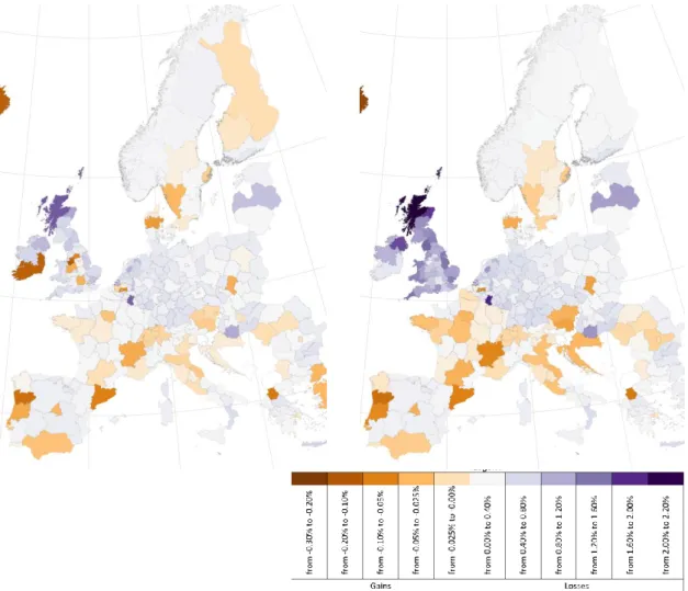
Figure 2 shows the overall losses of competitiveness per UK and EU region due to Brexit in the left hand side panel inclusive) and the international competitiveness (national-exclusive) effect only in the right hand side panel. As we see in Figure 2, again the overall national and regional losses of competitiveness for the UK regions are much higher than for other EU regions. Some regions in the Low Countries, Ireland, plus a small number of Central European regions also experience declines in competitiveness. The severe competitiveness shocks across much of the UK are a major concern for UK long-run national productivity, especially at a time when the UK is facing severe productivity challenges (McCann 2016). At the same time, many other regions of Europe actually gain in
competitiveness at the UK’s expense, precisely because of the UK’s decline in regional competitiveness.
Figure 2: Change of competitiveness in hard-Brexit scenario in EU regions (Left) and of international competitiveness only (Right)
When we consider only national-inclusive competition, we see in the left hand panel of Figure 2 that several regions in the UK actually gain relatively in competitiveness. The relative improvements in the positions of some regions, e.g. Cheshire, Greater Manchester and West Yorkshire, is at the expense of the worsening of the positions of other nearby regions in the UK. The same holds for regions in Ireland. This is because the competitiveness positions of regions not only relate to the direct and indirect cost effects itself, but also on these effects on competing (nearby) regions. In a hard-Brexit scenario, many UK-based firms will benefit from the direct increase in sales prices of EU competitors due to the imposed tariffs, but at the same time they will disproportionally lose out on the indirect value-chain
cost increases. As a result, some UK firms will increase their competitiveness in the UK-internal market, mainly at the expense of other UK firms that are even harder hit. In terms of international competitiveness though (Figure 2, right hand side), all UK regions lose out vis-à-vis non-UK EU regions, demonstrating that the competitiveness-redistribution effects within the UK are totally overshadowed by overall international competitive fall-out.
5. Uncertainty of Brexit Implications
Variations in the exact design of any post-Brexit UK-EU treaty lead to uncertainty in assessing the post-Brexit competitiveness implications for different regions and different
industries, such that there are different degrees of sensitivity to the variations of agreement
design faced by different regions. However, the method we introduced (in section 3) and applied (in section 4) allows us to map the regional degree of sensitivity or uncertainty of
Brexit impacts.Figure 3 shows the sensitivity to Brexit scenarios for Europe as a whole, and
Figure 4 focusses in on the UK.In terms of regional and sectoral implications, it is clear that
the largest impacted regions in the UK (and on the mainland in Germany) display only
limited sensitivity to the post-Brexit trade agreement design. In other words, no matter what
exactly eventually emerges as the design of the post-Brexit agreement, the adverse economic
effects will be relatively large in the UK. In the UK, Figure 4 shows that the economies of
London and of the larger Northern cities (Manchester, Liverpool, Edinburgh, Glasgow) however are relatively sensitive (more uncertain) of the implications of Brexit on their economies, while more peripheral regions are more certain of their (typically much more negative) implications. Thus, the larger cities have still a lot to gain (or rather potentially
greater reductions in losses of competiveness) from a ‘good’ Brexit deal. Meanwhile,
regional economies in France, Scandinavia, Spain, the Netherlands and Eastern Europe which are specialised in agricultural production and/or (traditional) manufacturing activities, are also rather sensitive to the Brexit design-scenario, whereas Belgian, Danish and German regions display little sensitivity to the design (Figure 3). Figures 2, 3 and 4 should be viewed simultaneously in order to compare the competiveness implications with the certainty of these
Figure 3: Sensitivity to Brexit Scenario for the EU
6. Regional and sectoral specificity
Given the detail in our data, the regional scores can also be decomposed into industry-region specific implications. Table 1 presents the combined competitiveness effects and cost increase effects (in brackets in cells) for selected regions and industries in the UK, and in The
Netherlands and the EU as a whole.7
The cost-increase effects can be substantial in region-industry combinations, but when other competing regions have larger cost-increasing effects, the relative competitiveness of regions can still improve due to Brexit. The deepening of greyed cells in Table 1 indicates whether changes in competitiveness depend on many different tariffs having a comparable effect (darker grey), or depend on only a few tariffs (lighter grey). In the former case the relative effect of Brexit on competitiveness will be relatively independent of the Brexit scenario, while in the latter case, the negotiated political Brexit scenario may have a strong effect on the actual effects of Brexit on competitiveness. It is this regional and sectoral specificity of the size of the effects in combination with the likeliness of this effect that is important for understanding the complexity of Brexit and providing local policymakers with the intelligence that is applicable to their situation.
To take as one example, Table 1 shows that the largest impacted industry in the UK is the motor-vehicle industry, with major competitiveness implications being very likely in the regions of the West-Midlands, Merseyside and East-Riding, and with a large competitiveness effects combined with a small sensitivity to tariffs, such that the automotive industries in these regions will be severely impacted on irrespective of what form of Brexit will become reality. The region of Cheshire, however, which is also home to a substantial automotive industry, actually gains in competitiveness in that specific industry because its sales are
largely UK-oriented8, but this relative competitiveness gain is largely at the expense of the
other UK car-producing regions which tend to be more export-oriented.
7 The full version for all UK and EU regions and industries is available on request 8
However, our analysis only considers trade and production cost effects and does not consider the intra-corporate global strategy implications. In this regard, on 22 January 2019 Bentley (VW) in Crewe issued a warning about the dangers of Brexit for their Cheshire facility (“Exclusive: No-Deal Brexit Puts Bentley’s Return to Profit at Risk”, Reuters 22/01/2019; uk.reuters.com) and there is also widespread concern about the long-term future of the Vauxhall Astra plant in Ellesmere Port (“Vauxhall Chief Warns of Brexit Threat to Ellesmere Port”, BBC News 06 March 2018; “Vauxhall Owner ‘could move Astra production from the UK’. BBC News 29 July 2019) owned by Group PSA the parent company of Peugeot-Citroën. In both of these cases these plants are part of much larger EU-based global automotive manufacturers with opportunities for plant relocation to regions with little or no adverse post-Brexit competiveness implications.
Table 1 : International competitiveness, cost changes and sensitivity to Brexit scenario in UK regions for selected industries
Grey in table: above average size sector (specialization) with divergent average certainty effect in the region. Dark grey: above average certainty of impact of Brexit (insensitive to the exact Brexit (non)tariff scenario). scenario. Light grey: below average certainty of impact of Brexit (sensitive to the exact Brexit (non)tariff scenario). Numbers: effect on competitiveness - a negative number is an improvement in competitiveness. The cost increase numbers are between brackets. Selection of sectors: at least one element/cell in the row should be grey.
EU Average NL Average UK Average Greater
Manchester Cheshire Merseyside East Riding and North Lincolnshire West Yorkshire Lincolnshire West Midlands Berkshire, Buckingham shire and Oxfordshire Average over all sectors 0.1 (0.4) 0.5 (0.8) 1 (1.7) 0.4 (1.3) 0.2 (1.5) 0.8 (2.2) 1 (2.9) 0.4 (1.4) 1 (3) 0.6 (1.7) 0.4 (1.5) Crop and animal production, hunting and related service activities -0.1 (0.5) 0.7 (1.6) 2.8 (6.6) 1.0 (6.1) -0.6 (4.8) 1.8 (6.9) 4.5 (7.0) 1.5 (6.1) 3.1 (7.0) 3.8 (7.6) 2.7 (7.2) Fishing and aquaculture -0.7 (0.2) -1.0 (1.9) 7.1 (8.2) 6.0 (6.9) 5.6 (6.5) 5.3 (6.1) 7.6 (9.3) 5.5 (6.5) 10.6 (11.9) 5.2 (6.2) 5.9 (6.9) Mining and quarrying 0.1 (0.1) 0.0 (0.0) 0.4 (0.5) 0.2 (0.4) 0.0 (0.3) 0.1 (0.3) 0.5 (0.7) 0.2 (0.4) 0.9 (1.1) 0.5 (0.7) 0.3 (0.5) Manufacture of food products; beverages and tobacco products 1.0 (1.3) 4.3 (5.5) -3.5 (3.9) -3.3 (3.1) -2.3 (2.5) -3.2 (3.1) -3.7 (6.4) -2.7 (4.8) -1.3 (7.5) -2.2 (5.6) -5.1 (4.2) Manufacture of textiles, wearing apparel, leather and related products 0.2 (0.3) 5.1 (6.0) 3.6 (3.1) 3.7 (6.0) 1.1 (2.2) 2.7 (4.3) 4.5 (6.9) 2.3 (4.1) 2.8 (4.5) 2.6 (4.4) 2.8 (4.4) Manufacture of coke and refined petroleum products 0.4 (0.4) 0.6 (0.4) 1.7 (2.9) 2.2 (4.7) 0.9 (3.6) -0.7 (2.0) 6.3 (8.7) 0.4 (3.4) 2.3 (5.2) 2.8 (5.3) 0.6 (3.3) Manufacture of chemicals and chemical products 0.6 (1.3) 0.7 (1.4) 1.7 (6.1) -1.2 (5.1) 0.5 (5.8) 0.8 (6.2) 2.0 (8.4) -2.2 (4.2) 5.4 (11.2) 0.1 (6.5) -2.4 (5.2) Manufacture of basic pharmaceutical products and pharmaceutical preparations 0.0 (0.3) 0.0 (0.3) 3.9 (1.2) 2.9 (3.9) -0.3 (0.7) 0.1 (0.5) 5.5 (6.4) 3.9 (4.8) 2.7 (3.6) 4.7 (5.7) 0.3 (1.3) Manufacture of rubber and plastic products 0.2 (1.0) -0.2 (1.0) 7.7 (7.7) 6.4 (11.1) 1.1 (6.1) 3.2 (7.7) 5.6 (11.6) 8.0 (12.5) 6.8 (12.3) 4.7 (10.1) 8.0 (12.4) Manufacture of basic metals 0.2 (0.4) 0.0 (0.4) 7.3 (3.9) 6.6 (8.5) 0.1 (2.6) 2.6 (4.3) 7.2 (9.2) 6.2 (8.2) 9.0 (10.7) 5.4 (7.4) 6.9 (8.7) Manufacture of fabricated metal products, except machinery and equipment 0.1 (0.2) 0.1 (0.4) 1.7 (1.8) 1.0 (2.1) 0.3 (1.5) 0.3 (1.4) 1.5 (3.0) 0.8 (2.0) 3.9 (5.0) 0.7 (1.7) 0.7 (2.0) Manufacture of computer, electronic and optical products 0.3 (0.7) 0.3 (0.6) 2.8 (1.5) 1.9 (3.3) -0.4 (0.8) -0.1 (1.1) 4.0 (5.3) 2.4 (3.8) 3.8 (5.2) 2.5 (4.0) 1.7 (3.3) Manufacture of machinery and equipment n.e.c. 0.2 (0.6) 0.0 (0.8) 5.1 (5.0) 3.9 (9.1) -0.2 (2.9) 1.4 (3.9) 6.7 (11.9) 4.5 (9.6) 6.1 (11.5) 3.3 (8.9) 3.2 (9.5) Manufacture of motor vehicles, trailers and semi-trailers -0.2 (2.2) -0.1 (1.1) 11.9 (12.8) 6.5 (14.5) 0.3 (8.1) 9.7 (15.8) 18.7 (26.0) 7.1 (15.6) 11.3 (19.1) 5.4 (13.6) 5.9 (15.2) Manufacture of other transport equipment 0.7 (1.4) 0.6 (1.3) 7.2 (6.2) 7.1 (10.7) 1.5 (4.4) 3.5 (6.3) 11.4 (16.1) 8.9 (12.6) 9.2 (13.4) 5.0 (9.0) 5.7 (10.0) Manufacture of furniture; other manufacturing 0.4 (0.8) 0.5 (0.9) 3.5 (1.7) 2.1 (4.5) -1.9 (1.1) -1.0 (1.7) 5.7 (8.6) 2.1 (4.7) 5.2 (8.0) 2.0 (5.0) 1.3 (4.7) Sewerage, waste management, remediation activities 0.1 (0.6) 0.1 (1.2) 0.1 (2.8) 0.9 (2.4) 0.3 (2.5) 1.1 (3.1) 0.2 (2.2) 0.4 (1.9) 0.5 (2.6) 0.2 (2.5) -1.1 (3.3) Wholesale trade, except of motor vehicles and motorcycles 0.1 (0.2) 0.8 (1.3) -2.6 (4.1) -0.3 (4.0) -0.1 (4.3) -0.8 (3.8) -5.9 (3.0) -1.5 (3.5) -4.7 (3.0) -1.7 (3.8) 0.4 (4.5) Retail trade, except of motor vehicles and motorcycles 0.2 (0.2) 0.8 (1.0) 1.1 (1.0) 1.0 (1.3) 0.2 (0.6) 0.6 (1.0) 0.8 (1.6) 0.8 (1.2) 1.4 (1.9) 1.0 (1.4) 0.9 (1.3) Land transport and transport via pipelines 0.1 (0.2) 0.2 (0.2) -0.1 (1.4) -0.3 (0.8) 0.8 (1.7) 0.8 (1.6) 0.4 (1.9) -0.2 (0.9) 0.2 (1.6) -0.4 (0.9) -0.5 (0.9) Water transport 0.5 (0.9) 0.3 (0.4) 0.2 (0.6) 0.3 (2.3) -2.2 (0.3) -1.8 (0.6) 0.5 (2.1) -1.8 (0.9) 8.3 (10.0) 1.8 (4.0) -0.5 (2.6) Warehousing and support activities for transportation -0.1 (0.1) 0.0 (0.1) 1.8 (1.8) 1.8 (2.0) 1.3 (1.5) 1.4 (1.6) 1.3 (1.8) 1.4 (1.7) 1.6 (2.1) 1.7 (2.0) 1.9 (2.2) Accommodation and food service activities 0.0 (0.3) -0.1 (0.2) 3.3 (2.5) 2.1 (2.6) 0.6 (1.5) 1.2 (2.1) 4.0 (4.7) 2.2 (2.7) 4.5 (5.2) 3.0 (3.7) 2.4 (3.6) Publishing activities -0.1 (0.3) -0.7 (0.5) 1.0 (1.6) 1.4 (1.9) 0.3 (1.1) 1.1 (1.9) 1.1 (1.5) 1.0 (1.5) 1.5 (1.9) 1.1 (1.8) 0.5 (1.9) Motion picture, video, television programme production; programming and broadcasting activities-0.3 (0.3) -0.9 (0.2) 1.2 (1.6) 1.2 (1.7) 0.5 (1.1) 1.4 (2.1) 1.1 (1.5) 1.0 (1.4) 1.5 (1.9) 1.1 (1.7) 0.7 (1.9) Telecommunications -0.1 (0.2) -0.3 (0.3) 1.3 (2.0) 1.5 (2.3) 0.7 (1.5) 1.2 (2.0) 1.4 (2.1) 1.1 (1.9) 1.9 (2.6) 1.3 (2.2) 1.0 (2.1) Financial service activities, except insurance and pension funding -0.1 (0.1) -0.3 (0.1) 1.0 (0.8) 1.0 (1.2) 0.9 (1.1) 1.0 (1.2) 0.8 (0.9) 1.0 (1.2) 1.0 (1.1) 0.9 (1.0) 0.8 (0.9) Insurance, reinsurance and pension funding, except compulsory social security 0.1 (0.2) 0.0 (0.1) 0.2 (0.5) 0.0 (0.3) -0.1 (0.4) 0.2 (0.7) 0.4 (0.9) 0.0 (0.3) 0.7 (1.2) 0.0 (0.3) 0.0 (0.4) Activities auxiliary to financial services and insurance activities -0.4 (0.2) -0.1 (0.1) 0.6 (1.7) 0.7 (1.1) 0.5 (0.9) 0.5 (0.9) 0.4 (0.7) 0.6 (1.0) 0.5 (0.8) 0.6 (0.9) 0.7 (1.0) Imputed rents of owner-occupied dwellings -0.1 (0.0) -0.1 (0.0) 0.7 (0.0) 0.6 (0.0) 0.6 (0.0) 0.8 (0.0) 0.5 (0.0) 0.5 (0.0) 0.7 (0.0) 0.6 (0.0) 0.7 (0.0) Scientific research and development 0.0 (0.1) 0.0 (0.1) 1.2 (2.2) 1.0 (1.8) 0.8 (2.4) 1.4 (2.1) 1.0 (1.6) 0.8 (1.4) 1.2 (1.9) 1.0 (1.7) 1.1 (1.8) Advertising and market research -0.2 (0.1) -0.9 (0.2) 1.7 (1.3) 1.6 (1.2) 1.6 (0.9) 2.0 (1.6) 1.3 (1.1) 1.2 (1.0) 1.7 (1.3) 1.5 (1.2) 1.6 (1.2) Other professional, scientific and technical activities; veterinary activities 0.1 (0.1) 0.1 (0.1) 0.9 (2.2) 0.9 (1.9) 0.1 (2.0) 0.5 (2.4) 1.3 (1.5) 0.8 (1.4) 1.4 (1.9) 0.9 (1.7) -0.1 (1.9) Travel agency, tour operator reservation service and related activities 0.0 (0.2) -0.2 (0.2) 1.1 (0.3) 0.9 (0.9) 0.5 (0.2) 0.9 (0.3) 1.0 (1.0) 0.8 (0.8) 1.2 (1.2) 0.9 (1.0) 1.0 (1.1) Residential care activities and social work activities without accommodation 0.1 (0.1) 0.1 (0.1) 0.0 (0.7) 0.2 (0.4) 0.2 (0.4) 1.1 (0.5) -0.1 (0.9) -0.1 (0.5) 0.8 (0.9) -0.4 (0.6) -0.4 (0.7)
Table 2: International competitiveness, cost changes and sensitivity to Brexit scenario in mainland EU regions for selected industries
Grey in table: above average size sector (specialization) with divergent average certainty effect in the region. Dark grey: above average certainty of impact of Brexit (insensitive to the exact Brexit (non)tariff scenario). scenario. Light grey: below average certainty of impact of Brexit (sensitive to the exact Brexit (non)tariff scenario). Numbers: effect on competitiveness - a negative number is an improvement in competitiveness. The cost increase numbers are between brackets. Selection of sectors: at least one element/cell in the row should be grey.
Zuid Holland Zeeland Vlaams Brabant
Île de
France Rhône-Alpes Norte Steiermark
Southern and Eastern
Ireland Cataluña Oberbayern Sydsverige
Average over all sectors 0.40 (0.9) 0.83 (1.7) -0.01 (0.5) -0.06 (0.0) -0.08 (0.7) -0.14 (0.1) -0.11 (0.9) 0.03 (0.3) -0.14 (0.0) 0.22 (0.0) -0.03 (0.0)
Crop and animal production, hunting and related service activities 1.0 (2.0) 1.2 (2.4) 0.5 (0.7) 0.0 (0.0) -0.1 (0.3) -0.1 (0.0) 0.0 (0.2) 0.2 (0.1) -0.5 (1.0) -0.3 (0.0) -0.8 (0.0)
Fishing and aquaculture 1.6 (3.0) 0.3 (2.9) -1.6 (0.5) -0.7 (0.0) -0.8 -(100.0) -0.3 (0.1) -0.1 (0.2) 0.0 (0.1) -0.9 (3.0) 0.0 (0.0) -0.4 (0.0)
Mining and quarrying -0.1 (0.0) 0.0 (0.0) 0.3 (0.3) 0.8 (0.0) 0.1 (0.5) 0.1 (0.9) 0.0 (0.1) 0.4 (0.0) 0.1 (0.0) 0.1 (0.0) 0.0 (0.0)
Manufacture of food products; beverages and tobacco products 8.9 (11.8) 7.9 (10.7) -1.5 (1.5) 0.0 (0.0) 0.0 (0.5) 0.0 (0.1) 0.0 (5.2) 0.4 (0.3) -0.1 (4.0) 3.7 (0.0) 0.1 (0.0)
Manufacture of textiles, wearing apparel, leather and related products 1.3 (5.8) 11.1 (14.0) -3.7 (1.1) 0.0 (0.0) 0.0 (0.2) 0.0 (0.1) 0.0 (0.1) 0.2 (0.1) 0.0 (5.0) 0.0 (0.0) -0.2 (0.0)
Manufacture of coke and refined petroleum products 1.1 (1.5) 1.0 (1.5) 0.1 (0.3) -0.1 (0.0) 0.1 (0.8) 0.0 (0.0) -0.2 (0.2) 0.5 (0.2) -0.1 (0.0) -0.5 (0.0) 0.0 (0.0)
Manufacture of chemicals and chemical products 0.3 (0.9) 0.8 (1.9) 0.6 (1.5) 0.0 (0.0) -0.3 (0.5) 0.0 (0.1) -0.2 (2.3) -0.7 (0.0) 0.0 (0.0) 1.2 (0.0) -0.1 (0.0)
Manufacture of basic pharmaceutical products and pharmaceutical preparations 0.1 (0.4) 0.2 (0.5) 0.1 (0.4) -0.1 (0.0) -0.1 (0.4) 0.0 (0.1) -0.1 (0.2) 0.2 -(100.0) 0.0 (0.0) 0.1 (0.0) 0.0 (0.0)
Manufacture of rubber and plastic products -0.1 (1.3) 0.6 (2.5) -0.5 (1.3) -0.6 (0.0) -0.4 (2.8) -0.3 (0.5) -0.4 (0.5) -2.1 (1.3) -0.5 (0.0) -0.5 (0.0) -0.3 (0.0)
Manufacture of basic metals -0.2 (0.3) 0.0 (0.6) 0.5 (1.2) -0.2 (0.0) -0.2 (0.6) 0.4 (0.2) -0.2 (0.7) -1.0 (1.0) 0.2 (0.0) 0.2 (0.0) 0.2 (0.0)
Manufacture of fabricated metal products, except machinery and equipment 0.1 (0.3) 0.4 (0.7) 0.3 (0.5) 0.0 (0.0) 0.0 (1.0) 0.0 (0.2) 0.0 (0.2) -1.3 (0.2) 0.0 (0.0) 0.0 (0.0) 0.0 (0.0)
Manufacture of computer, electronic and optical products 0.3 (0.7) 0.4 (1.0) 0.1 (0.6) -0.1 (0.0) 0.0 (2.7) 0.1 (0.1) -0.1 (0.2) 1.7 (1.2) -0.2 (0.0) 0.0 (0.0) 0.4 (0.0)
Manufacture of machinery and equipment n.e.c. 0.3 (1.0) 0.0 (1.1) 0.2 (1.2) -0.1 (0.0) -0.2 (1.8) -0.3 (0.1) -0.1 (0.6) -0.5 (1.0) -0.1 (0.0) 0.3 (0.0) 0.2 (0.0)
Manufacture of motor vehicles, trailers and semi-trailers 0.7 (5.0) 1.9 (12.1) 0.4 (5.0) -0.8 (0.0) -1.5 (1.4) -0.9 (0.3) -0.6 (2.5) -2.8 (5.8) -1.1 (0.0) 0.4 (0.0) 0.1 (0.0)
Manufacture of other transport equipment 0.2 (0.9) 2.6 (5.5) -0.2 (0.8) -0.1 (0.0) -0.5 (1.4) -1.5 (0.3) 0.1 (0.5) -0.5 (4.9) 0.6 (0.0) -0.3 (0.0) 2.7 (0.0)
Manufacture of furniture; other manufacturing 0.2 (0.8) 1.0 (1.9) 0.2 (0.7) -0.5 (0.0) -0.5 -(100.0) -0.7 (0.1) 0.2 (0.7) 0.0 (1.0) -0.8 (0.0) 0.3 (0.0) 0.3 (0.0)
Sewerage, waste management, remediation activities 0.3 (1.2) 0.3 (1.0) 0.6 (2.0) -0.5 (0.0) -0.6 (0.3) -0.8 (0.1) -0.1 (0.4) -0.3 (0.8) -0.6 (0.0) -0.3 (0.0) 0.3 (0.0)
Wholesale trade, except of motor vehicles and motorcycles 0.6 (1.4) 1.3 (2.8) 0.3 (0.5) 0.0 (0.0) 0.0 (0.6) 0.0 (0.0) 0.0 (0.3) -2.3 (0.1) 0.0 (0.0) 0.1 (0.0) 0.0 (0.0)
Retail trade, except of motor vehicles and motorcycles 0.7 (1.1) 2.2 (2.7) 0.0 (0.4) 0.0 (0.0) 0.0 (0.5) -0.6 -(100.0) -0.1 (0.2) -4.4 (0.0) -0.5 (0.0) 0.0 (0.0) -0.2 (0.0)
Land transport and transport via pipelines 0.0 (0.0) 0.6 (1.0) -0.3 (0.2) -0.2 (0.0) 0.0 (0.7) 0.5 (0.0) -0.1 (0.1) -1.7 (0.0) -0.1 (0.0) -0.1 (0.0) -0.2 (0.0)
Water transport 0.0 (0.1) 0.2 (0.4) 0.2 (0.2) 0.0 (0.0) 0.1 (2.1) 0.0 (0.1) 2.0 (0.3) 1.3 (0.1) 1.5 (0.0) 0.2 (0.0) 0.0 (0.0)
Warehousing and support activities for transportation -0.1 (0.1) 0.2 (0.4) -0.1 (0.2) -0.2 (0.0) -0.2 (0.4) -0.4 (0.1) -0.1 (0.2) 0.3 (0.1) -0.1 (0.0) -0.2 (0.0) -0.2 (0.0)
Accommodation and food service activities -0.3 (0.1) 0.1 (0.5) 0.8 (1.4) -0.1 (0.0) -0.1 (0.7) -0.9 (0.0) -0.1 (0.6) -2.1 (0.0) -0.5 (0.0) 0.0 (0.0) -0.1 (0.0)
Publishing activities 0.0 (0.5) -2.0 (0.4) -0.2 (0.7) -0.2 (0.0) -0.1 -(100.0) -1.1 (0.1) -0.1 (0.2) 0.0 (0.3) -0.3 (0.0) 0.0 (0.0) 0.0 (0.0)
Motion picture, video, television programme production; programming and broadcasting activities-0.3 (0.4) -2.2 (1.1) -0.1 (0.2) -0.2 (0.0) -0.5 (0.9) -2.4 (0.1) -0.3 (0.2) 0.7 (0.6) -0.3 (0.0) 0.0 (0.0) -0.2 (0.0)
Telecommunications -0.1 (0.1) -1.1 (0.9) -0.5 (0.4) -0.1 (0.0) -0.1 (0.7) -1.1 (0.1) -0.1 (0.3) -1.0 (0.3) -0.4 (0.0) 0.0 (0.0) -0.3 (0.0)
Financial service activities, except insurance and pension funding -0.1 (0.1) -0.5 (0.5) -0.2 (0.1) -0.1 (0.0) -0.2 (0.3) -0.2 (0.0) -0.1 (0.1) 0.1 (0.0) -0.1 (0.0) -0.5 (0.0) 0.0 (0.0) Insurance, reinsurance and pension funding, except compulsory social security -0.1 (0.1) 0.2 (0.3) 0.1 (0.2) -0.1 (0.0) -0.1 (0.2) -0.4 (0.0) -0.3 (0.1) 0.2 (0.4) 0.3 (0.0) 0.0 (0.0) 0.2 (0.0) Activities auxiliary to financial services and insurance activities -0.3 (0.0) 0.0 (0.2) 0.0 (0.2) -0.2 (0.0) -0.2 (0.6) -0.3 (0.0) -0.1 (0.2) 0.4 (0.0) -1.2 (0.0) -0.5 (0.0) -0.2 (0.0)
Imputed rents of owner-occupied dwellings -0.1 (0.0) -0.1 (0.0) 0.0 (0.0) 0.0 (0.0) -0.1 (0.0) 0.0 (0.0) -0.1 (0.0) 0.5 (0.0) 0.0 (0.0) -0.1 (0.0) -0.2 (0.0)
Scientific research and development -0.2 (0.1) 0.6 (0.1) 0.1 (0.2) -0.1 (0.0) -0.1 (0.8) 0.6 (0.1) 0.0 (0.0) -0.7 (0.0) -0.1 (0.0) -0.1 (0.0) 0.0 (0.0)
Advertising and market research -0.8 (0.1) -2.4 (1.2) -0.3 (0.3) -0.1 (0.0) 0.0 (0.2) -0.3 (0.0) -0.1 (0.0) -0.7 (0.1) -0.1 (0.0) -0.3 (0.0) -0.1 (0.0)
Other professional, scientific and technical activities; veterinary activities 0.1 (0.1) 0.3 (0.5) 0.1 (0.2) 0.0 (0.0) 0.1 (0.7) 0.0 (0.1) 0.0 (0.1) 0.8 (0.1) 0.1 (0.0) -0.1 (0.0) 0.0 (0.0) Travel agency, tour operator reservation service and related activities -0.2 (0.2) 0.0 (0.4) -0.3 (0.4) -0.1 (0.0) -0.1 (1.0) 0.0 (0.0) -0.1 (0.0) 0.0 (0.1) -0.1 (0.0) -0.1 (0.0) 0.0 (0.0) Residential care activities and social work activities without accommodation 0.0 (0.0) 0.3 (0.1) 0.1 (0.1) 0.1 (0.0) 0.1 -(100.0) -0.2 (0.0) -0.3 (0.0) -0.1 (0.0) -0.2 (0.0) 0.2 (0.0) 0.2 (0.0)
The Cheshire automotive industry faces an only’ an 8 percent cost increase, compared to 14 and 16 percent increases in Birmingham and East-Riding, respectively. However, once we also include the international competition, then as with all other UK regions, the region of Cheshire also loses out vis-à-vis competitors in Germany and other specialized car producing regions in the world.
Other examples in Table 1 show that relatively certain (tariff-insensitive) impacts are in the computer and optical manufacturing in Oxford, and the machinery and equipment manufacturing industries of Birmingham, Liverpool and West-Yorkshire. Food production generally gains in competitiveness in the UK with little uncertainty. UK services, which tend to be concentrated in larger cities, are sensitive to the post-Brexit scenario and can be impacted when a hard Brexit scenario is applied, although many services (except for The City of London financial markets) are barely discussed in the negotiations between the UK and the
EU.9
What is immediately apparent from the top line of Table 1 is that the loss of competitiveness in the UK is about ten times larger than the EU as a whole due to the reductions in cross-border competition and the increase in both direct and indirect cost increases. At the same time, the loss of competitiveness in the UK compared to The Netherlands appears to be only
2 times higher.10 The reason is that a great deal of competition is with competitors that also
face cost increases. The absolute effects, also in competitiveness terms, are large, with an average relative cost increases of 1 percent. The higher costs for UK firms is caused by the higher dependency on cross-border value-chains, almost all of which will be affected by cost increases, whereas most of The Netherlands’ value-chains remain unaffected by Brexit. In other words, the Brexit hit to UK competitiveness is borne largely by the UK’s firms and industries which are heavily engaged in UK-EU trade, the same firms which are essential for driving the UK’s overall productivity agenda. At the same time, UK consumers will pay for a large share of the costs since the relative cost effect on UK firms is much smaller than the absolute cost effect. This gives UK firms the possibility to pass on a large part of the cost increase to UK consumers in the form of higher retail prices.
Comparable to Table 1, Table 2 presents the combined competitiveness effects and cost increase effects (in brackets in cells) for selected regions and industries in mainland Europe.
9
Note that in Table 1 the degree of uncertainty is calculated from the perspective of the region. This implies mathematically that high or low uncertainty is determined relative to the average uncertainty over the sectors in the region.
10