Manual for Dynamic Modelling of Soil Response to Atmospheric Deposition

(1)

pReport 259101012/2003

Manual for Dynamic Modelling

of Soil Response to Atmospheric Deposition

M Posch, J-P Hettelingh, J Slootweg (eds)

ICP M&M Coordination Center for Effects

wge

Working Group on Effects

of the

(2)

This investigation has been performed by order and for the account of the Directorate for Climate Change and Industry of the Dutch Ministry of Housing, Spatial Planning and the Environment within the framework of MNP project M259101, ‘UNECE-CLRTAP’; and for the account of the Working Group on Effects within the trustfund for the partial funding of effect oriented activities under the Convention.

(3)

Preface

At the first Expert Workshop on Dynamic Modelling (Ystad, Sweden, 3-5 Oct. 2000) the ICP on Modelling and Mapping was ‘urged’ to draft a ‘Modelling Manual’ (UNECE 2001a). A first draft of such a Modelling Manual has been presented at the CCE Workshop (Bilthoven, The Netherlands, April 2001) and the Task Force meeting of the ICP on Modelling and Mapping (Bratislava, Slovakia, May 2001), at which it was recommended to modify the Manual and distribute it for further comments. Further drafts were discussed at the 2nd and 3rd meeting of the Joint Expert Group (JEG) on Dynamic Modelling (Ystad, 6-8 Nov. 2001 and Sitges, Spain, 6-8 Nov. 2002). Its advice, and the advice from several other readers, was taken into account in the preparation of the Manual.

Acknowledgements

The CCE would like to acknowledge the contributions of many individuals. Foremost among them W. de Vries from Alterra (Wageningen, The Netherlands), who inter alia wrote Chapter 5 of this Manual. Thanks also to R. Wright from (NIVA, Norway) for providing the description of the MAGIC model and the contribution on recovery of aquatic ecosystems. Also the input of H. Sverdrup (Univ. Lund, Sweden) during (informal) meetings at the CCE (and elsewhere) is gratefully acknowledged. Last, but not least, we would like to thank all readers, especially Julian Aherne (Trent Univ., Ontario, Canada), who provided valuable comments on earlier drafts of this Manual.

(4)

(5)

Abstract

The objective of this manual is to inform the network of National Focal Centres (NFCs) about the requirements of methodologies for the dynamic modelling of geochemical processes, especially in soils. This information is necessary to support European air quality policies with knowledge on time delays of ecosystem damage or recovery caused by changes, over time, of acidifying deposition.

This Manual has been requested by bodies under the Convention on Long-range Transboundary Air Pollution (CLRTAP) to support the extension of the European critical load database with dynamic modelling parameters.

A Very Simple Dynamic (VSD) model is described to encourage NFCs to meet minimum data requirements upon engaging in the extension of national critical load databases. This manual can be consulted in combination with a running version of VSD, which is available on www.rivm.nl/cce. The report also provides an overview of existing dynamic models, which generally require more input data.

Finally, the manual tentatively describes possible linkages between dynamic modelling results and integrated assessment modelling. This linkage is necessary for use in the near future support of the policy review of the 1999 CLRTAP Protocol to Abate Acidification, Eutrophication and Ground-level Ozone (the ‘Gothenburg Protocol’) and the 2001 EU National Emission Ceiling Directive.

(6)

(7)

Samenvatting

Dit rapport informeert het netwerk van National Focal Centra (NFCs) over de vereisten van methodologiën voor de gevolgtijdelijke (dynamische) modellering van geochemische processen, vooral in bodems. Deze informatie is nodig om het Europese luchtbeleid te kunnen ondersteunen met kennis over tijdsvertragingen van ecosysteemherstel of -schade als gevolg van veranderingen, in de tijd, van verzurende depositie.

Het is geschreven op verzoek van werkgroepen onder de Conventie van Grootschalige Grensoverschrijdende Luchtverontreiniging (CLRTAP). Dit ter ondersteuning van de uitbreiding met dynamische modelparameters van de Europese databank die momenteel uitsluitend kritische waarden voor verzurende en vermestende deposities bevat.

Een Very Simple Dynamic (VSD) model wordt beschreven teneinde NFCs aan te moedigen om te voldoen aan minimale databehoeften bij de uitbreiding van nationale databanken van kritische waarden. De handleiding kan worden geraadpleegd in combinatie met het gebruik van een geïmplementeerde versie van het VSD model dat beschikbaar is op www.rivm.nl/cce. De handleiding geeft ook een overzicht van bestaande dynamische modellen die doorgaans meer complexe databehoeften hebben.

Tenslotte verschaft het rapport een eerste beschrijving van mogelijke verbindingen tussen resultaten van dynamische modellering en geïntegreerde modellen voor de ondersteuning van luchtbeleid (Integrated Assessment Models). Deze zijn in de nabije toekomst nodig voor de ondersteuning van de beleidsmatige evaluatie van het 1999 CLRTAP Protocol voor de bestrijding van verzuring, vermesting en troposferische ozon (het Gotenburg protocol) en de EU-richtlijn 2001/81/EG van het Europese Parlement (2001) inzake nationale emissieplafonds voor bepaalde luchtverontreinigende stoffen (NEC directive).

(8)

(9)

Summary

Dynamic modelling is the logical extension of steady-state critical loads in support of the effects-oriented work under the Convention on Long-range Transboundary Air Pollution (CLRTAP). European data bases and maps of critical loads have been used to support effects-based Protocols to the CLRTAP, such as the 1994 Protocol on Further Reduction of Sulphur Emissions (the ‘Oslo Protocol’) and the 1999 Protocol to Abate Acidification, Eutrophication and Ground-level Ozone (the ‘Gothenburg Protocol’). Critical loads are based on a steady-state concept, they are the constant depositions an ecosystem can tolerate in the long run, i.e. after it has equilibrated with these depositions.

However, many ecosystems are not in equilibrium with present or projected depositions, since there are processes (‘buffer mechanisms’) at work, which delay the reaching of an equilibrium (steady state) for years, decades or even centuries. By definition, critical loads do not provide any information on these time scales. Therefore, in its 17-th session in December 1999, the Executive Body of the Convention ‘... underlined the importance of ... dynamic modelling of recovery’ (ECE/EB.AIR/68 p. 14, para. 51. b) to enable the assessment of time delays of recovery in regions where critical loads cease being exceeded and time delays of damage in regions where critical loads continue to be exceeded.

The objective of this Manual is to inform the network of National Focal Centres (NFCs) about the requirements of methodologies for the dynamic modelling of soil and water chemistry. This information has been requested by bodies under the CLRTAP to support the extension of the European critical load database with dynamic modelling parameters. A Very Simple Dynamic (VSD) model is described to encourage NFCs to meet minimum data requirements upon engaging in the extension of national critical load databases. This manual can be read in combination with a running version of VSD, which is available on www.rivm.nl/cce. The manual also provides an overview of existing dynamic models which generally require more input data.

Finally, the manual describes possible linkages between dynamic modelling results and integrated assessment modelling via so-called target load functions. Such a linkage is necessary the future support of the review of the 1999 CLRTAP Gothenburg Protocol and the 2001 EU National Emission Ceiling Directive.

(10)

(11)

1 Introduction

The critical load concept has been developed in Europe since the mid-1980s, mostly under the auspices of the 1979 Convention on Long-range Transboundary Air Pollution (LRTAP). European data bases and maps of critical loads have been instrumental in formulating effects-based Protocols to the LRTAP Convention, such as the 1994 Protocol on Further Reduction of Sulphur Emissions (the ‘Oslo Protocol’) and the 1999 Protocol to Abate Acidification, Eutrophication and Ground-level Ozone (the ‘Gothenburg Protocol’).

Critical loads are based on a steady-state concept, they are the constant depositions an ecosystem can tolerate in the long run, i.e. after it has equilibrated with these depositions. However, many ecosystems are not in equilibrium with present or projected depositions, since there are processes (‘buffer mechanisms’) at work, which delay the reaching of an equilibrium (steady state) for years, decades or even centuries. By definition, critical loads do not provide any information on these time scales. Therefore, in its 17-th session in December 1999, the Executive Body of the Convention ‘... underlined the importance of ... dynamic modelling of recovery’ (UNECE 1999).

Dynamic models are not new. For 15-20 years scientists have been developing, testing and applying dynamic models to simulate the acidification of soils or surface waters, mostly due to the deposition of sulphur. But it is a relatively new topic for the effects-oriented work under the LRTAP Convention. Earlier work, e.g. under the ICP on Integrated Monitoring, has applied existing dynamic models at a few sites for which sufficient input data are available. The new challenge is to develop and apply dynamic model(s) on a European scale and to combine them as much as possible with the integrated assessment work under the LRTAP Convention, in support of the review and potential revision of protocols.

This Manual aims at providing information for the National Focal Centres (NFCs) of the ICP on Modelling and Mapping and their collaborating institutes on the concepts and data requirements for dynamic modelling. It should assist them in providing information on dynamic model inputs and results to the Coordination Center for Effects (CCE), if and when requested by the Working Group on Effects (WGE). This Manual is not a user manual for running any existing dynamic model. Rather, it focuses on those aspects of dynamic modelling relevant to the work under the LRTAP Convention in general and its application in integrated assessment in particular. An important constraint in this context is that any dynamic modelling output generated for this purpose has to be consistent with results from critical loads modelling. For example, in areas, where critical loads were never exceeded, dynamic models should not identify the need for further deposition reductions. With these constraints in mind, this Manual provides a description of basic principles and equations underlying essentially all dynamic soil models as well as the (minimum) input data requirements. Emphasis is placed on consistency and compatibility with the Simple Mass Balance (SMB) model for calculating critical loads. An important part of this Manual is the discussion of the links with integrated assessment (modelling), since this is the main context in which dynamic modelling results will be used under the framework of the LRTAP Convention. It is the hope of the compilers of this Manual that it will do what the Mapping Manual did for critical loads: To help creating common procedures and data bases which can be used in future negotiations on emission reductions of sulphur and nitrogen.

(14)

The organisation of the Manual is as follows. Chapter 2 explains the reasons for dynamic modelling in the framework of the Convention on LRTAP as a next step following the assessment of European critical loads and summarises the possible use of dynamic modelling results in integrated assessment. Chapter 3 focuses on the basic concepts and related equations of dynamic modelling and the underlying treatment of finite buffer processes influencing the long-term temporal development of critical limits. Chapter 4 provides a short overview of existing widely used dynamic models, including relevant literature references. Chapter 5 discusses input data and calibration requirements of dynamic models with emphasis on the variables for which data are needed in addition to those needed for critical load calculations. Chapter 6 discusses the problems encountered when calculating target loads and lists a number of options for presenting dynamic modelling results, with emphasis on methods for presenting results on a regional scale. Finally, some special (technical) topics are treated in several Annexes.

(15)

2 Dynamic Modelling in Support of Protocol

Negotiations

The purpose of this Chapter is to explain and motivate the use (and constraints) of dynamic modelling as a natural extension of critical loads in support of the effects-oriented work under the LRTAP Convention.

2.1 Why dynamic modelling?

In the Mapping Manual (UBA 1996) the methodologies for calculating critical loads for use under the LRTAP Convention have been documented. Dynamic models have been discussed in workshops of the ICP on Modelling and Mapping since 1989, and the Mapping Manual contains a short section on dynamic modelling (pp.116-121), which mostly summarises the characteristics of some widely used dynamic models. The present Manual can be seen as an extension of that section in the Mapping Manual. For the sake of simplicity and in order to avoid the somewhat vague term ‘ecosystem’, we refer in the sequel to non-calcareous (forest) soils. However, most of the considerations hold for surface water systems as well, since their water quality is strongly influenced by properties of and processes in catchment soils. A separate report dealing with the dynamic modelling of surface waters on a regional scale has been prepared under the auspices of the ICP Waters (Jenkins et al. 2002).

In the causal chain from deposition of strong acids to damage to key indicator organisms there are two major links that can give rise to delays. Biogeochemical processes can delay the chemical response in soil, and biological processes can further delay the response of indicator organisms, such as damage to trees in forest ecosystems. The static models to determine critical loads consider only the steady-state condition, in which the chemical and biological response to a (new) (constant) deposition is complete. Dynamic models, on the other hand, attempt to estimate the time required for a new (steady) state to be achieved. With critical loads, i.e. in the steady-state situation, only two cases can be distinguished when comparing them to deposition: (1) the deposition is below critical load(s), i.e. does not exceed critical loads, and (2) the deposition is greater than critical load(s), i.e. there is critical load exceedance. In the first case there is no (apparent) problem, i.e. no reduction in deposition is deemed necessary. In the second case there is, by definition, an increased risk of damage to the ecosystem. Thus a critical load serves as a warning as long as there is exceedance, since it states that deposition should be reduced. However, it is often assumed that reducing deposition to (or below) critical loads immediately removes the risk of ‘harmful effects’, i.e. the chemical criterion (e.g. the Al/Bc-ratio1_{) that links the critical load}

to the (biological) effect(s), immediately attains a non-critical (‘safe’) value and that there is immediate biological recovery as well. But the reaction of soils, especially their solid phase, to changes in deposition is delayed by (finite) buffers, the most important being the cation exchange capacity (CEC). These buffer mechanisms can delay the attainment of a critical

1_{In the Mapping Manual (and elsewhere) the Bc/Al-ratio is used. However, this ratio becomes}

infinite when the Al concentration approaches zero. To avoid this inconvenience, its inverse, the Al/Bc-ratio, is used here.

(16)

chemical parameter, and it might take decades or even centuries, before an equilibrium (steady state) is reached. These finite buffers are not included in the critical load formulation, since they do not influence the steady state, but only the time to reach it. Therefore, dynamic models are needed to estimate the times involved in attaining a certain chemical state in response to deposition scenarios, e.g. the consequences of ‘gap closures’ in emission reduction negotiations. In addition to the delay in chemical recovery, there is likely to be a further delay before the ‘original’ biological state is reached, i.e. even if the chemical criterion is met (e.g. Al/Bc<1), it will take time before biological recovery is achieved. Figure 1 summarises the possible development of a (soil) chemical and biological variable in response to a ‘typical’ temporal deposition pattern. Five stages can be distinguished:

Stage 1: Deposition was and is below the critical load (CL) and the chemical and

biological variables do not violate their respective criteria. As long as deposition stays below the CL, this is the ‘ideal’ situation.

Stage 2: Deposition is above the CL, but (chemical and) biological criteria are not

violated because there is a time delay before this happens. No damage is likely to occur at this stage, therefore, despite exceedance of the CL. The time between the first exceedance of the CL and the first violation of the biological criterion (the first occurrence of actual damage) is termed the Damage Delay Time (DDT=t3-t1).

Stage 3: The deposition is above the CL and both the chemical and biological criteria

are violated. Measures (emission reductions) have to be taken to avoid a (further) deterioration of the ecosystem status.

Stage 4: Deposition is below the CL, but the (chemical and) biological criteria are still

violated and thus recovery has not yet occurred. The time between the first non-exceedance of the CL and the subsequent non-violation of both criteria is termed the Recovery Delay Time (RDT=t6-t4).

Stage 5: Deposition is below the CL and both criteria are no longer violated. This stage

is similar to Stage 1 and only at this stage can the ecosystem be considered to have recovered. Stages 2 and 4 can be subdivided into two sub-stages each: Chemical delay times (DDTc=t2-t1 and RDTc=t5-t4; dark grey in Figure 1) and (additional) biological delay times (DDTb=t3-t2 and RDTb=t6-t5; light grey). Very often, due to the lack of operational biological response models (but see Annex A), damage and recovery delay times mostly refer to chemical recovery alone and this is used as a surrogate for overall recovery.

In addition to the large number of dynamic model applications to individual sites over the past 15 years, there are several examples of early applications of dynamic models on a (large) regional scale. Earlier versions of the RAINS model (Alcamo et al. 1990) contained an effects module which simulated soil acidification on a European scale (Kauppi et al. 1986) and lake acidification in the Nordic countries (Kämäri and Posch 1987). Cosby et al. (1989) applied the MAGIC dynamic lake acidification model to regional lake survey data in southern Norway, and Evans et al. (2001) used the same model to study freshwater acidification and recovery in the United Kingdom. Alveteg et al. (1995) and SAEFL (1998) used the SAFE model to assess temporal trends in soil acidification in southern Sweden and Switzerland. De Vries et al. (1994) employed the SMART model to simulate soil acidification in Europe, and Hettelingh and Posch (1994) used the same model to investigate recovery delay times on a European scale.

(17)

Stage 1 Stage 2 Stage 3 Stage 4 Stage 5 Acid deposition Critical Load Chemical response (Al/Bc)crit Biological response critical response time t1 t2 t3 t4 t5 t6 DDT RDT

Figure 1: ‘Typical’ past and future development of the acid deposition effects on a soil chemical

variable (Al/Bc-ratio) and the corresponding biological response in comparison to the critical values of those variables and the critical load derived from them. The delay between the (non)exceedance of the critical load, the (non)violation of the critical chemical criterion and the crossing of the critical biological response is indicated in grey shades, highlighting the Damage Delay Time (DDT) and the Recovery Delay Time (RDT) of the system.

The dynamic modelling concepts and data requirements presented in the following are an extension of those employed in deriving the Simple Mass Balance (SMB) model. The SMB model is described in detail in the Mapping Manual. Earlier descriptions of the SMB model can be found in Sverdrup et al. (1990), De Vries (1991), Sverdrup and De Vries (1994) and Posch et al. (1995). The most basic extension of the SMB model into a dynamic soil acidification model are realised in the Very Simple Dynamic (VSD) model, which is described in Posch and Reinds (2003).

2.2 Steady state and dynamic models

Steady-state models (critical loads) have been used to negotiate emission reductions in Europe. An emission reduction will be judged successful if non-exceedance of critical loads is attained. To gain insight into the time delay between the attainment of non-exceedance and actual chemical (and biological) recovery, dynamic models are needed. Thus the dynamic models to be used in the assessment of recovery under the LRTAP Convention have to be compatible with the steady-state models used for calculating critical loads. In other words, when critical loads are used as input to the dynamic model, the (chemical) parameter chosen as the criterion in the critical load calculation has to attain the critical value (after the dynamic simulation has reached steady state). But this also means that

(18)

concepts and equations used in the dynamic model have to be an extension of the concepts and equations employed in deriving the steady-state model. For example, if critical loads are calculated with the Simple Mass Balance (SMB) model, the steady-state version of the dynamic model used has to be the SMB (e.g. the SMART model). Analogously, if the SAFE model is used for dynamic simulations, critical loads have to be calculated with the steady-state PROFILE model; etc.

Most likely, due to a lack of (additional) data and other resources, it will be impossible to run dynamic models on all sites in Europe for which critical loads are calculated at present (about 1.5 million). However, the selection of the subset or sub-regions of sites, at which dynamic models are applied in support of integrated assessments, has to be representative enough to allow comparison with results obtained with critical loads.

Dynamic models of acidification are based on the same principles as steady-state models: The charge balance of the ions in the soil solution, mass balances of the various ions, and equilibrium equations. However, whereas in steady-state models only infinite sources and sinks are considered (such as base cation weathering), the inclusion of the finite sources and sinks of major ions into the structure of dynamic models is crucial, since they determine the long-term (slow) changes in soil (solution) chemistry. The three most important processes involving finite buffers and time-dependent sources/sinks are cation exchange, nitrogen retention and sulphate adsorption.

Cation exchange is characterised by two quantities: cation exchange capacity (CEC), the total number of exchange sites (a soil property), and base saturation, the fraction of those sites occupied by base cations at any given time. After an increase in acidifying input, cation exchange (initially) delays the decrease in the acid neutralisation capacity (ANC) by releasing base cations from the exchange complex, thus delaying the acidification of the soil solution until a new equilibrium is reached (at a lower base saturation). On the other hand, cation exchange delays recovery since ‘extra’ base cations are needed to replenish base saturation instead of increasing the ANC of the soil solution. Detailed discussions and early model formulations of cation exchange reactions in the context of soil acidification can be found in Reuss (1980, 1983) and Reuss and Johnson (1986).

Finite nitrogen sinks: In the calculation of critical loads the net input of nitrogen is assumed constant over time or, in case of denitrification, a function of the (constant) N deposition. However, it is well known that the amount of N immobilised is in most cases larger than the long-term sustainable (‘acceptable’) immobilisation rate used in critical load calculations. Observational and experimental evidence (e.g. Gundersen et al. 1998a) shows a correlation between the C/N-ratio and the amount of N retained in the soil organic layer. This correlation can been used to formulate simple models of N immobilisation in which the amount of N retained is a function of the prevailing C/N-ratio, which in turn is updated by the amount retained. Such an approach is described below and used in the SMART model (De Vries et al. 1994), the MERLIN model (Cosby et al. 1997) and in version 7 of the MAGIC model (Cosby et al. 2001).

Sulphate adsorption can be an important process in some soils for regulating sulphate concentration in the soil solution. Equilibrium between dissolved and adsorbed sulphate in the soil/soilwater system is typically described by a Langmuir isotherm, which is characterised by two parameters: The maximum adsorption capacity and the ‘half-saturation constant’, which determines the speed of the response to changes in sulphate concentration. A description and extensive model experiments can be found in Cosby et al. (1986).

(19)

2.3 Use of dynamic models in Integrated Assessment

Ultimately, within the framework of the LRTAP Convention, a link has to be established between the dynamic soil models and integrated assessment (models) used in the Task Force on Integrated Assessment Modelling (TFIAM). The following modes of interaction with integrated assessment (IA) models can be identified:

Scenario analyses:

Deposition scenario output from IA models are used by the ‘effects community’ (ICPs) as input to dynamic models to analyse their impact on (European) soils and surface waters, and the results (recovery times etc.) are reported back to the ‘IA community’.

Presently available dynamic models are well suited for this task. The question is how to summarise the resulting information on a European scale. Also, the ‘turn-around time’ of such an analysis, i.e. the time between obtaining deposition scenarios and reporting back dynamic model results, is bound to be long within the framework of the LRTAP Convention.

Response functions for optimisation (e.g. target load functions):

Response functions are derived with dynamic models and linked to IA models. Such response functions encapsulate a site’s temporal behaviour to reach a certain (chemical) state in response to a broad range of (future) deposition patterns; or they characterise the amount of deposition reductions needed to obtain a certain state within a prescribed time. In the first case these response functions are pre-processed model runs for a large number of plausible future deposition patterns from which the results for every (reasonable) deposition scenario can be obtained by interpolation. A first attempt in this direction has been presented by Alveteg et al. (2000); and an example is shown in Figure 2. It shows the isolines of years (‘recovery isochrones’) in which Al/Bc<1 is attained for the first time for a given combination of percent deposition reduction (vertical axis) and implementation year (horizontal axis). The reductions are expressed as percentage of the deposition in 2010 after implementation of the Gothenburg Protocol and the implementation year refers to the full implementation of that additional reduction. For example, a 48% reduction of the 2010 deposition, fully implemented by the year 2030 will result in a (chemical) recovery by the year 2060 (dashed line in Figure 2). Note that for this example site, at which critical loads are still exceeded after implementation of the Gothenburg Protocol, no recovery is possible unless further reductions exceed 32% of the 2010 level.

(20)

2020 2030 2040 2050 2060 2080 2100 2150

No recovery

2010 2030 2050 2070 2090 2110 8 16 24 32 40 48 56 64 72 80 88 96 Year of implementation

% Dep-reduction beyond G-Protocol

Figure 2: Example of ‘recovery isochrones’. The vertical axis gives the additional reduction in

acidifying deposition after the implementation of the Gothenburg Protocol in 2010 (expressed as percentage of the 2010 level) and the horizontal axis the year at which this additional reductions are fully implemented. The isolines are labelled with the first year at which Al/Bc<1 is attained for a given combination of percent reduction and implementation year.

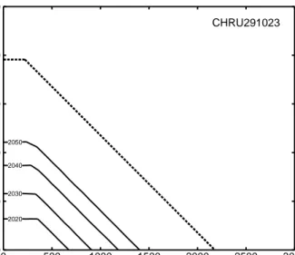
Considering how critical loads have been used in IA during the negotiations of protocols, it is unlikely that there will be much discussion about the implementation year of a new reduction agreement (mostly 5-10 years after a protocol enters into force). Thus the question will be: What is the maximum deposition allowed to obtain (and sustain!) a desired chemical state (e.g. Al/Bc=1) in a prescribed year? In the case of a single pollutant, this can be read from information as presented in Figure 2. However, in the case of acidity, both N and S deposition determine the soil chemical state. In addition, it will not be possible to obtain unique pairs of Nand Sdeposition to reach a prescribed target (compare critical load function for acidity critical loads). Thus, dynamic models are used to determine target loads functions for a series of target years. These target load functions, or suitable statistics derived from them, are passed on to the IA-modellers who evaluate their feasibility of achievement (in terms of costs and technological abatement options available). In Figure 3 examples of target load functions are shown for a set of target years.

The determination of target load functions (or any other type of response functions) requires no changes to existing models per se, but rather additional work, since dynamic soil model have to run many times and/or ‘backwards’, i.e. in an iterative mode. A further discussion of the problems and possible pitfalls in the computation of target load functions can be found in Chapter 6.

(21)

2020 2030 2040 2050 0 500 1000 1500 2000 2500 3000 0 500 1000 1500 2000 2500 Ndep (eq ha-1yr-1) Sdep (eq ha -1yr -1) CHRU291023

Figure 3: Examples of target load functions for 4 different target years (2020-2050). Also shown is

the critical load function of the site (thick dashed line). Note that any target load function has to lie below the critical load function, i.e. requires stricter deposition reductions than achieving critical load.

Integrated dynamic model:

A dynamic model could be integrated into the IA models (e.g. RAINS) and used in scenario analyses and optimisation runs. The widely used models, such as MAGIC, SAFE and SMART, are not easily incorporated into IA models, and they might be still too complex to be used in optimisation runs. Alternatively, the VSD model could be incorporated into the IA models, capturing the essential, long-term features of dynamic soil models. This would be comparable to the process that led to the simple ozone model included in RAINS, which was derived from the complex photo-oxidant model of EMEP. However, even this would require a major effort, not the least of which is the creation of a European database to run the model.

2.4 Constraints for dynamic modelling under the LRTAP

Convention

The request of the Executive Body for dynamic model applications is aimed in particular at regions where critical loads are exceeded even after the implementation of the Gothenburg Protocol. For these regions policy questions include when damage becomes irreversible or how additional emission reductions can be best phased in. But also regions where exceedances no longer occur are of interest. In such regions policy questions include when recovery is achieved (see also Warfvinge et al. 1992). Therefore, an important constraint for the application of dynamic modelling is that the input database for a European application – including the chosen critical limit(s) – is compatible with the input data for critical loads submitted by NFCs. Otherwise dynamic model applications may not result in the same regional patterns of exceedances, which would be highly confusing for the review process of the Gothenburg Protocol. On the other hand, the extension of the current critical load database to enable the application of dynamic models provides an excellent opportunity to review and update national critical load databases.

(22)

(23)

3 Basic Concepts and Equations

In this chapter we present the basic concepts and equations common to virtually all dynamic (soil) models and discuss the underlying simplifying assumptions. The guiding principle is the compatibility with critical load models, since the steady-state solutions of the dynamic model employed should be the critical loads.

In addition to chemical criteria, which have been used to set critical loads and will thus be used to define/judge recovery, also the biological response has to be considered. And although models for that are largely lacking, some ideas are presented in Annex A.

3.1 Basic equations

As mentioned above, we consider as ‘ecosystem’ non-calcareous forest soils, although most of the considerations hold also for non-calcareous soils covered by (semi-)natural vegetation. Since we are interested in applications on a large regional scale (for which data are scarce) and long time horizons (decades to centuries with a time step of one year), we assume that the soil is a single homogeneous compartment and its depth is equal to the root zone. This implies that internal soil processes (such as weathering and uptake) are evenly distributed over the soil profile, and all physico-chemical constants are assumed uniform in the whole profile. Furthermore we assume the simplest possible hydrology: The water leaving the root zone is equal to precipitation minus evapotranspiration; more precisely, percolation is constant through the soil profile and occurs only vertically. These are the same assumptions made when deriving critical loads with the Simple Mass Balance (SMB) model.

As for the SMB model, the starting point is the charge balance of the major ions in the soil water, leaching from the root zone:

(3.1) SO4,_le+NO3,_le−NH4,_le−BC_le+Cl_le =H_le+Al_le−HCO3,_le−RCOO_le=−ANC_le where BC=Ca+Mg+K+Na and RCOO stands for the sum of organic anions. Eq.3.1 also defines the acid neutralising capacity, ANC. The leaching term is given by Xle=Q[X] where [X] is the soil solution concentration (eq/m3) of ion X and Q (m/yr) is the water percolating from the root zone (precipitation minus evapotranspiration). All quantities are expressed in equivalents (moles of charge) per unit area and time (e.g. eq/m2/yr).

The concentration [X] of an ion in the soil compartment, and thus its leaching Xle in the charge balance, is related to the sources and sinks of X via a mass balance equation, which describes the change over time of the total amount of ion X per unit area in the soil matrix/soil solution system, Xtot (eq/m2):

(3.2)

X

_tot

X

_net

X

_le

dt

d

−

=

where Xnet (eq/m2/yr) is the net input of ion X (sources minus sinks, except leaching), which are specified and discussed below.

(24)

With the simplifying assumptions used in the derivation of the SMB model, the net input of sulphate and chloride is given by their respective deposition:

(3.3)

SO

₄_,_net

=

S

_dep

and

Cl

_net

=

Cl

_dep

For base cations the net input is given by (Bc=Ca+Mg+K, BC=Bc+Na): (3.4)

BC

_net

=

BC

_dep

+

BC

_w

−

Bc

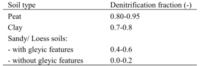
_u

where the subscripts dep, w and u stand for deposition, weathering and net uptake, respectively. Note, that S adsorption and cation exchange reactions are not included here, they are included in Xtot and described by equilibrium equations (see below). For nitrate and ammonium the net input consists of (at least) deposition, nitrification, denitrification, net uptake and immobilisation:

(3.5)

NO

₃_,_net

=

NO

_x_,_dep

+

NH

₄_,_ni

−

NO

₃_,_i

−

NO

₃_,_u

−

NO

₃_,_de

(3.6)

NH

₄_,_net

=

NH

₃_,_dep

−

NH

₄_,_ni

−

NH

₄_,_i

−

NH

₄_,_u

where the subscripts ni, i and de stand for nitrification, net immobilisation and denitrification, respectively. In the case of complete nitrification one has NH4,net=0 and the net input of nitrogen is given by:

(3.7)

NO

3,_net

=

N

_net

=

N

_dep

−

N

_i

−

N

_u

−

N

_de

In addition to the mass balances, equilibrium equations describe the interaction of the soil solution with air and the soil matrix. The dissolution of (free) Al is modelled by the following equation:

(3.8)

[

Al

]

=

KAl

_ox

[

H

]

α

where α>0 is a site-dependent exponent. For α=3 this is the familiar gibbsite equilibrium (KAlox=Kgibb).

Bicarbonate ions were neglected in the derivation of the SMB model since for low pH-values related to the critical limit for forest soils the resulting error was considered negligible. But they can as easily be included: The bicarbonate concentration, [HCO3], is computed as

(3.9)

]

[

]

[

1 2 3

H

p

K

HCO

₌

H CO

where K1 is the first dissociation constant, KH is Henry's constant (K1KH=10−1.7=0.02 eq2/m6/atm at 8oC) and pCO2 (atm) is the partial pressure of CO2 in the soil solution. Note that the inclusion of bicarbonates into the charge balance is necessary, if the ANC is to attain positive values.

(25)

Also organic anions have been neglected in the critical load calculations, the assumption being that all organic anions are complexed with aluminium, i.e. free Al is equal to total Al minus organic anions. But as long as they are modelled by equilibrium equations with [H] their inclusion does not pose any difficulty.

Thus the ANC-concentration can be expressed as a function of [H] alone (see eq.3.1):

(3.10)

]

[

]

[

]

[

]

[

]

[

]

[

]

[

])

([

])

([

4 2 1

Cl

N

SO

BC

H

KAl

H

p

K

H

F

H

ANC

H CO _ox org

−

=

−

+

=

α

where Forg is a function expressing organic anion concentration(s) in terms of [H].

3.2 Finite buffer processes

Finite buffers have not been included in the derivation of critical loads, since they do not influence the steady state. However, when investigating the chemistry of soils over time as a function of changing deposition patterns, these finite buffers govern the long-term (slow) changes in soil (solution) chemistry. These finite buffers include adsorption/desorption processes, mineralisation/immobilisation processes and dissolution/precipitation processes, and in the following we discuss them in turn.

3.2.1 Sources and sinks of cations

Cation exchange:

Generally, the solid phase particles of a soil carry an excess of cations at their surface layer. Since electro-neutrality has to be maintained, these cations cannot be removed from the soil, but they can be exchanged against other cations, e.g. those in the soil solution. This process is known as cation exchange; and every soil (layer) is characterised by the total amount of exchangeable cations per unit mass (weight), the so-called cation exchange capacity (CEC, measured in meq/kg). If X and Y are two cations with charges m and n, then the general form of the equations used to describe the exchange between the liquid-phase concentrations (or activities) [X] and [Y] and the equivalent fractions EX and EY at the exchange complex is

(3.11) _n _m n m XY j Y i X

Y

X

K

E

]

[

]

[

+ +

=

where KXY is the so-called exchange (or selectivity) constant, a soil-dependent quantity. Depending on the powers i and j different models of cation exchange can be distinguished: For i=n and j=m one obtains the Gaines-Thomas exchange equations, whereas for i=j=mn, after taking the mn-th root, the Gapon exchange equations are obtained.

The number of exchangeable cations considered depends on the purpose and complexity of the model. For example, Reuss (1983) considered only the exchange between Al and Ca (or divalent base cations). In general, if the exchange between N ions is considered, N-1, exchange equations (and constants) are required, all the other (N-1)(N-2)/2 relationships

(26)

and constants can be easily derived from them. In the VSD model the exchange between aluminium, divalent base cations and protons is considered. The exchange of protons is important, if the cation exchange capacity (CEC) is measured at high pH-values (pH=6.5). In the case of the Bc-Al-H system, the Gaines-Thomas equations read:

(3.12)

]

[

]

[

and

]

[

]

[

2 2 2 3 2 2 3 3 2 + + + +

=

Bc

H

K

E

Bc

Al

K

E

HBc Bc H AlBc Bc Al

where Bc=Ca+Mg+K, with K treated as divalent. The equation for the exchange of protons against Al can be obtained from eqs.3.12 by division:

(3.13) _HAl _HAl _HBc _AlBc

Al H

_K

Al

H

K

E

/

with

]

[

]

[

3 3 3 3

=

+₊

The corresponding Gapon exchange equations read:

(3.14) ₂ ₁_/₂ ₂ ₁_/₂ 3 / 1 3

]

[

]

[

and

]

[

]

[

+ + + +

=

Bc

H

k

E

Bc

Al

k

E

HBc Bc H AlBc Bc Al

Again, the H-Al exchange can be obtained by division (with kHAl=kHBc/kAlBc). Charge balance requires that the exchangeable fractions add up to one:

(3.15)

E

Bc

+

E

Al

+

E

H

=

1

The user of the VSD model can choose between the Gaines-Thomas and the Gapon Bc-Al-H exchange model. The sum of the fractions of exchangeable base cations (here EBc) is called the base saturation of the soil; and it is the time development of the base saturation, which is of interest in dynamic modelling. In the above formulations the exchange of Na, NH4 (which can be important in high NH4 deposition areas) and heavy metals is neglected (or subsumed in the proton fraction).

Care has to be exercised when comparing models, since different sets of exchange equations are used in different models. Whereas eqs.3.12 are used in the SMART model (but with Ca+Mg instead of Bc, K-exchange being ignored in the current version), the SAFE model employs the Gapon exchange equations (eqs.3.14), however with exchange constants k’X/Y=1/kXY. In the MAGIC model the exchange of Al with all four base cations is modelled separately with Gaines-Thomas equations, without explicitly considering H-exchange. In Chapter 5 ranges of values for the exchange constants for the different model formulations are presented.

3.2.2 Sources and sinks of nitrogen

Mineralisation and immobilisation:

Several models do include descriptions for mineralisation and immobilisation, following e.g. first order kinetics or Michaelis-Menten kinetics. For those descriptions we refer to the respective models. In its most simple form, a net immobilisation of nitrogen is included, being the difference between mineralisation and immobilisation.

(27)

In the calculation of critical loads the (acceptable, sustainable) long-term net immobilisation Ni,acc, is assumed to be constant and not influencing the C/N-ratio, i.e. a proportional amount of C is assumed to be immobilised. However, it is well known, that the amount of N immobilised is (at present) in many cases larger than this long-term value. Thus a submodel describing the nitrogen dynamics in the soil is part of most dynamic models. For example, the MAKEDEP model (Alveteg et al. 1998a, Alveteg and Sverdrup 2002), which is part of the SAFE model system (but can also be used as a stand-alone routine) describes the N-dynamics in the soil as a function of forest growth and deposition.

According to Dise et al. (1998) and Gundersen et al. (1998b) the forest floor C/N-ratios may be used to assess risk for nitrate leaching. Gundersen et al. (1998b) suggested threshold values of >30, 25 to 30, and <25 to separate low, moderate, and high nitrate leaching risk, respectively. This information has been used in several models, such as SMART (De Vries et al. 1994, Posch and De Vries 1999) and MAGIC (Cosby et al. 2001) to calculate nitrogen immobilisation as a fraction of the net N input, linearly depending on the C/N-ratio. In these models, the C/N-ratio of the mineral topsoil is used.

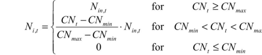
Between a maximum, CNmax, and a minimum C/N-ratio, CNmin, the net amount of N immobilised is a linear function of the actual C/N-ratio, CNt:

(3.16)

ï

î

ïï

í

ì

≤

<

⋅

−

≥

=

min t max t min t in min max min t max t t in t i

CN

N

CN

N

for

0 for

for

, , ,

where Nin,t is the available N (e.g., Nin,t=Ndep,t-Nu,t-Ni,acc). At every time step the amount of immobilised N is added to the amount of N in the top soil, which in turn is used to update the C/N-ratio. The total amount immobilised at every tine step is then Ni=Ni,acc+Ni,t. The above equation states that when the C/N-ratio reaches a (pre-set) minimum value, the annual amount of N immobilised equals the acceptable value Ni,acc (see Figure 4). This formulation is compatible with the critical load formulation for t→¥.

0 50 100 150 200 250 300 0 0.1 0.2 0.3 0.4 0.5 0.6 0.7 years Ni (eq/m 2/yr) 0 50 100 150 200 250 300 0 5 10 15 20 25 30 years C:N ratio

Figure 4: Amount of N immobilised (left) and resulting C/N-ratio in the topsoil (right) for a constant

net input of N of 1 eq/m2_{/yr (initial C}

pool=5 kgC/m2).

It should be noted that eq.3.16 does not capture all the features of observed (and expected!) behaviour of nitrogen immobilisation in soils, such as ‘sudden breakthrough’ after saturation, and more research is needed in this area.

(28)

3.2.3 Sources and sinks of sulphur

Mineralisation and immobilisation:

Several models do include descriptions for mineralisation and immobilisation, following e.g. first order kinetics or Michaelis-Menten kinetics. For those descriptions, refer to the respective models. In its most simplified form, a net immobilisation of sulphur is included, being the difference between mineralisation and immobilisation, which, in turn, is generally set to zero.

Sulphate adsorption:

The amount of sulphate adsorbed, SO4,ad (meq/kg), is often assumed to be in equilibrium with the solution concentration and is typically described by a Langmuir isotherm (e.g., Cosby et al. 1986): (3.17) _ad

S

_max

SO

S

SO

⋅

+

=

]

[

]

[

4 2 / 1 4 , 4

where Smax is the maximum adsorption capacity of sulphur in the soil (meq/kg) and S1/2 the half saturation concentration (eq/m3).

3.3 Critical limits

Chemical criteria:

Using the equations given in section 3.1 the leaching of ANC from the bottom of the root zone can be calculated for any given deposition. However, critical loads are derived by setting a certain soil chemical variable, which connects soil solution chemistry to a ‘harmful effect’ (the chemical ‘criterion’), and by solving the equation ‘backwards’ to obtain allowable deposition values. The various chemical criteria are summarised in the Mapping Manual and the most frequently used ones are given in Table 1.

Table 1: Most frequently used chemical criteria (used to derive critical loads).

Element Soil solution Surface water

Acidity Al/(Ca+Mg+K) < 0.5-2.0 [ANC] > 0-0.05 eq.m-3

Nitrogen [N] < 0.02-0.04 eq.m-3 _{[N] < 0.16 mol.m}-3

Finite buffers, such as cation exchange capacity, are not considered in the derivation of critical loads, since they do not influence steady-state situations. However, this does not mean that the state of those buffers is not influenced by the steady state! The relationship between the base saturation (i.e. the fraction of exchangeable base cations) and the soil chemical variables usually used in critical load calculations, e.g. the Al/Bc-ratio, can be easily derived (see Annex B). This also allows base saturation to be used as a chemical criterion in critical load calculations, as recommended at a recent workshop (Hall et al. 2001, UNECE 2001b).

(29)

Biological response models:

The abiotic models described above focus on the delays between changes in acid deposition and changes in soil and/or surface water chemistry. But there are also delays between changes in chemistry and the biological response. Since the goal of deposition reductions is to restore healthy and sustainable populations of key indicator organisms, the time lag in response is the sum of the delays in chemical and biological response (see also the discussion for Figure 1). Consequently, dynamic models for biological response are needed; and information about such models is given in Annex A, including both steady-state models (regression relationships) and process-oriented dynamic response models.

3.4 From steady state (critical loads) to dynamic simulations

3.4.1 Steady-state calculations

Steady state means there is no change over time in the total amounts of ions involved, i.e. (see eq.3.2): (3.18)

X

_tot

X

_le

X

_net

dt

d

=

Þ

= 0

From eq.3.5 the critical load of nutrient nitrogen, CLnut(N), is obtained by specifying an acceptable N-leaching, Nle(acc). By specifying a critical leaching of ANC, ANCle(crit), and inserting eqs.3.3-3.5 into the charge balance (eq.3.1), one obtains the equation describing the critical load function of S and N acidity, from which the three quantities CLmax(S), CLmin(N) and CLmax(N) can be derived (see Mapping Manual).

3.4.2 Dynamic calculations

To obtain time-dependent solutions of the mass balance equations, the term Xtot in eq.3.2, i.e. the total amount (per unit area) of ion X in the soil matrix/soil solution system has to be specified. For ions, which do not interact with the soil matrix, Xtot is given by the amount of ion X in solution alone:

(3.19)

X

_tot

=

Θ

z

[X

]

where z (m) is the soil depth under consideration (root zone) and Θ (m3_/m3_{) is the (annual} average) volumetric water content of the soil compartment. The above equation holds for chloride. For every base cation Y participating in cation exchange, Ytot is given by:

(3.20)

Y

_tot

=

Θ

z

[

Y

]

+

ρ

zCEC

⋅

E

_Y

where ρ is the soil bulk density (g/cm3_{), CEC the cation exchange capacity (meq/kg) and E}

Y is the exchangeable fraction of ion Y.

(30)

For nitrogen an update of the C/N-ratio is needed in those models which use that ratio in calculating N immobilisation. In this case, Ntot is given as:

(3.21)

N

_tot

=

Θ

z

[

N

]

+

ρ

zN

_soil

If there is no ad/desorption of sulphate, SO4,tot is given by eq.3.19. If sulphate adsorption cannot be neglected, it is given by (see eq.3.17):

(3.22)

SO

₄_,_tot

=

Θ

z

[

SO

₄

]

+

_ρ

zSO

₄_,_ad

Inserting these expressions into eq.3.2 and observing that Xle=Q[X], one obtains differential equations for the temporal development of the concentration of the different ions. Only in the simplest cases can these equations be solved analytically. In general, the mass balance equations are discretised and solved numerically, with the solution algorithm dependent on the model builders’ preferences.

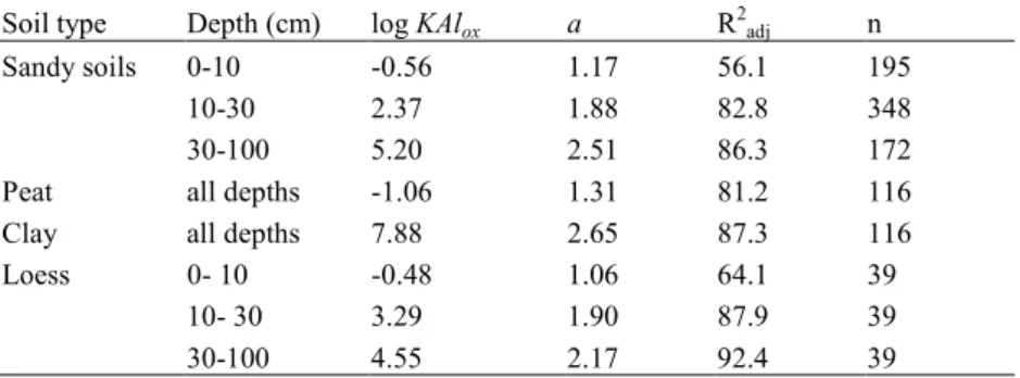
When the rate of Al leaching is greater than the rate of Al mobilisation by weathering of primary minerals, the remaining part of Al has to be supplied from readily available Al pools, such as Al hydroxides. This causes depletion of these minerals, which might induce an increase in Fe buffering which in turn leads to a decrease in the availability of phosphate (De Vries 1994). Furthermore, the decrease of those pools in podzolic sandy soils may cause a loss in the structure of those soils. The amount of aluminium is in most models assumed to be infinite and thus no mass balance for Al is considered. The SMART model, however, includes an Al balance, and the terms in eq.3.2 are Alnet=Alw and Altot is given by

(3.23)

Al

_tot

=

Θ

z

[

Al

]

+

CEC

_a

E

_Al

+

ρ

zAl

_ox

where Alox (meq/kg) is the amount of oxalate extractable Al, the pool of readily available Al in the soil.

(31)

4 Available Dynamic Models

In the previous sections the basic processes involved in soil acidification have been summarised and expressed in mathematical form, with emphasis on slow (long-term) processes. The resulting equations, or generalisations and variants thereof, together with appropriate solution algorithms and input-output routines have over the past 15 years been packaged into soil acidification models, mostly known by their (more or less fancy) acronyms.

There is no shortage of soil (acidification) models, but most of them are not designed for regional applications. A comparison of 16 models can be found in a special issue of the journal ‘Ecological Modelling’ (Tiktak and Van Grinsven 1995). These models emphasise either soil chemistry (such as SMART, SAFE and MAGIC) or the interaction with the forest (growth). There are very few truly integrated forest-soil models. An example is the forest model series ForM-S (Oja et al. 1995), which is implemented not in a ‘conventional’ Fortran code, but is realised in the high-level modelling software STELLA.

The following selection is biased towards models which have been (widely) used and which are simple enough to be applied on a (large) regional scale. Only a short description of the models can be given, but details can be found in the references cited. It should be emphasised that the term ‘model’ used here refers, in general, to a model system, i.e. a set of (linked) software (and databases) which consists of pre-processors for input data (preparation) and calibration, post-processors for the model output, and – in general the smallest part – the actual model itself. An overview of the various models is given in Table 2. The first three models are soil models of increasing complexity, whereas the MAGIC model is generally applied at the catchment level. Application on the catchment level, instead on a single (forest) plot, has implications for the derivation of input data. E.g., weathering rates have to represent the average weathering of the whole catchment, data that is difficult to obtain from soil parameters. Thus in MAGIC catchment weathering is calibrated from water quality data.

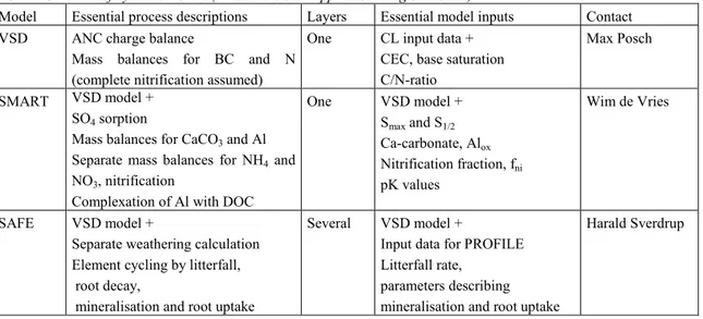
Table 2: Overview of dynamic models (which have been applied on a regional scale).

Model Essential process descriptions Layers Essential model inputs Contact VSD ANC charge balance

Mass balances for BC and N (complete nitrification assumed)

One CL input data + CEC, base saturation C/N-ratio

Max Posch

SMART VSD model + SO4 sorption

Mass balances for CaCO3 and Al

Separate mass balances for NH4 and

NO3, nitrification

Complexation of Al with DOC

One VSD model + Smax and S1/2 Ca-carbonate, Alox Nitrification fraction, fni pK values Wim de Vries SAFE VSD model +

Separate weathering calculation Element cycling by litterfall, root decay,

mineralisation and root uptake

Several VSD model +

Input data for PROFILE Litterfall rate,

parameters describing mineralisation and root uptake

(32)

MAGIC VSD model + SO4 sorption Al speciation/complexation Aquatic chemistry Several(m ostly one) VSD model + Smax and S1/2

pK values for several Al reactions

parameters for aquatic chemistry

Dick Wright

4.1 The VSD model

The basic equations presented in Chapter 3 have been used to construct a Very Simple Dynamic (VSD) soil acidification model. The VSD model can be viewed as the simplest extension of the SMB model for critical loads. It only includes cation exchange and N immobilisation, and a mass balance for cations and nitrogen as described above, in addition to the equations included in the SMB model. It resembles the model presented by Reuss (1980) which, however, does not consider nitrogen processes.

In the VSD model, the various ecosystem processes have been limited to a few key processes. Processes that are not taken into account, are: (i) canopy interactions, (ii) nutrient cycling processes, (iii) N fixation and NH4 adsorption, (iv) interactions (adsorption, uptake, immobilisation and reduction) of SO4, (v) formation and protonation of organic anions, (RCOO) and (vi) complexation of Al with OH, SO4 and RCOO.

The VSD model consists of a set of mass balance equations, describing the soil input-output relationships, and a set of equations describing the rate-limited and equilibrium soil processes, as described in Section 3. The soil solution chemistry in VSD depends solely on the net element input from the atmosphere (deposition minus net uptake minus net immobilisation) and the geochemical interaction in the soil (CO2 equilibria, weathering of carbonates and silicates, and cation exchange). Soil interactions are described by simple rate-limited (zero-order) reactions (e.g. uptake and silicate weathering) or by equilibrium reactions (e.g. cation exchange). It models the exchange of Al, H and Ca+Mg+K with Gaines-Thomas or Gapon equations. Solute transport is described by assuming complete mixing of the element input within one homogeneous soil compartment with a constant density and a fixed depth. Since VSD is a single layer soil model neglecting vertical heterogeneity, it predicts the concentration of the soil water leaving this layer (mostly the rootzone). The annual water flux percolating from this layer is taken equal to the annual precipitation excess. The time step of the model is one year, i.e. seasonal variations are not considered. A detailed description of the VSD model can be found in Posch and Reinds (2003).

4.2 The SMART model

The SMART model (Simulation Model for Acidification's Regional Trends) is similar to the VSD model, but somewhat extended and is described in De Vries et al. (1989) and Posch et al. (1993). As with the VSD model, the SMART model consists of a set of mass balance equations, describing the soil input-output relationships, and a set of equations describing the rate-limited and equilibrium soil processes. It includes most of the assumptions and simplifications given for the VSD model; and justifications for them can be found in De Vries et al. (1989). SMART models the exchange of Al, H and divalent base cations using

(33)

Gaines-Thomas equations. Additionally, sulphate adsorption is modelled using a Langmuir equation (as in MAGIC) and organic acids can be described as mono-, di- or tri-protic. Furthermore, it does include a balance for carbonate and Al, thus allowing the calculation from calcareous soils to completely acidified soils that do not have an Al buffer left. In this respect, SMART is based on the concept of buffer ranges expounded by Ulrich (1981). Recently a description of the complexation of aluminium with organic acids has been included. The SMART model has been developed with regional applications in mind, and an early example of an application to Europe can be found in De Vries et al. (1994).

4.3 The SAFE model

The SAFE (Soil Acidification in Forest Ecosystems) model has been developed at the University of Lund (Warfvinge et al. 1993) and a recent description of the model can be found in Alveteg (1998) and Alveteg and Sverdrup (2002). The main differences to the SMART and MAGIC models are: (a) weathering of base cations is not a model input, but it is modelled with the PROFILE (sub-)model, using soil mineralogy as input (Warfvinge and Sverdrup 1992); (b) SAFE is oriented to soil profiles in which water is assumed to move vertically through several soil layers (usually 4), (c) Cation exchange between Al, H and (divalent) base cations is modelled with Gapon exchange reactions, and the exchange between soil matrix and the soil solution is diffusion limited. The standard version of SAFE does not include sulphate adsorption although a version, in which sulphate adsorption is dependent on sulphate concentration and pH has recently been developed (Martinson et al. 2003).

The SAFE model has been applied to many sites and more recently also regional applications have been carried out for Sweden (Alveteg and Sverdrup 2002) and Switzerland (SAEFL 1998, Kurz et al. 1998, Alveteg et al. 1998b).

4.4 The MAGIC model

MAGIC (Model of Acidification of Groundwater In Catchments) is a lumped-parameter model of intermediate complexity, developed to predict the long-term effects of acidic deposition on soils and surface water chemistry (Cosby et al. 1985a,b,c, 1986). The model simulates soil solution chemistry and surface water chemistry to predict the monthly and annual average concentrations of the major ions in lakes and streams. MAGIC represents the catchment with aggregated, uniform soil compartments (one or two) and a surface water compartment that can be either a lake or a stream. MAGIC consists of (1) a section in which the concentrations of major ions are assumed to be governed by simultaneous reactions involving sulphate adsorption, cation exchange, dissolution-precipitation-speciation of aluminium and dissolution-dissolution-precipitation-speciation of inorganic and organic carbon, and (2) a mass balance section in which the flux of major ions to and from the soil is assumed to be controlled by atmospheric inputs, chemical weathering inputs, net uptake in biomass and losses to runoff. At the heart of MAGIC is the size of the pool of exchangeable base cations in the soil. As the fluxes to and from this pool change over time owing to changes in atmospheric deposition, the chemical equilibria between soil and soil solution shift to give changes in surface water chemistry. The degree and rate of change in surface water acidity thus depend both on flux factors and the inherent characteristics of the affected soils.

(34)

The soil layers can be arranged vertically or horizontally to represent important vertical or horizontal flowpaths through the soils. If a lake is simulated, seasonal stratification of the lake can be implemented. Time steps are monthly or yearly. Time series inputs to the model include annual or monthly estimates of: (1) deposition (wet plus dry) of ions from the atmosphere; (2) discharge volumes and flow routing within the catchment; (3) biological production, removal and transformation of ions; (4) internal sources and sinks of ions from weathering or precipitation reactions; and (5) climate data. Constant parameters in the model include physical and chemical characteristics of the soils and surface waters, and thermodynamic constants. The model is calibrated using observed values of surface water and soil chemistry for a specified period.

MAGIC has been modified and extended several times from the original version of 1984. In particular organic acids have been added to the model (version 5; Cosby et al. 1995) and most recently nitrogen processes have been added (version 7; Cosby et al. 2001).

The MAGIC model has been extensively applied and tested over a 15-year period at many sites and in many regions around the world. Overall, the model has proven to be robust, reliable and useful in a variety of scientific and managerial activities.

Manual for Dynamic Modelling of Soil Response to Atmospheric Deposition