research for man and environment
RIJKSINSTITUUT VOOR VOLKSGEZONDHEID EN MILIEU
NATIONAL INSTITUTE OF PUBLIC HEALTH AND THE ENVIRONMENT
RIVM report 481505020
Technical Report on Methodology: Cost
Benefit Analysis and Policy Responses
D.W. Pearce, A. Howarth
May 2000
This Report has been prepared by RIVM, EFTEC, NTUA and IIASA in association with
TME and TNO under contract with the Environment Directorate-General of the European
Commission.
Abstract
The economic assessment of priorities for a European environmental policy plan focuses on twelve identified Prominent European Environmental Problems such as climate change, chemical risks and biodiversity. The study, commissioned by the European Commission (DG Environment) to a European consortium led by RIVM, provides a basis for priority setting for European environmental policy planning in support of the sixth Environmental Action Programme as follow-up of the current fifth Environmental Action Plan called ‘Towards Sustainability’. The analysis is based on an examination of the cost of avoided damage, environmental expenditures, risk assessment, public opinion, social incidence and sustainability. The study incorporates information on targets, scenario results, and policy options and measures including their costs and benefits.
Main findings of the study are the following. Current trends show that if all existing policies are fully implemented and enforced, the European Union will be successful in reducing pressures on the environment. However, damage to human health and ecosystems can be substantially reduced with accelerated policies. The implementation costs of these additional policies will not exceed the environmental benefits and the impact on the economy is manageable. This requires future policies to focus on least-cost solutions and follow an integrated approach. Nevertheless, these policies will not be adequate for achieving all policy objectives. Remaining major problems are the excess load of nitrogen in the ecosystem, exceedance of air quality guidelines (especially particulate matter), noise nuisance and biodiversity loss.
This report is one of a series supporting the main report: European Environmental Priorities: an Integrated Economic and Environmental Assessment. The areas discussed in the main report are fully documented in the various Technical reports. A background report is presented for each environmental issue giving an outline of the problem and its relationship to economic sectors and other issues; the benefits and the cost-benefit analysis; and the policy responses. Additional reports outline the benefits methodology, the EU enlargement issue and the macro-economic consequences of the scenarios.
RIVM report 481505020 - 3 –
Technical Report on Methodology: Cost Benefit Analysis and Policy Responses
This report has been prepared by RIVM, EFTEC, NTUA and IIASA in association with TME and TNO under contract with the Environment Directorate-General of the European Commission. This report is one of a series supporting the main report titled European
Environmental Priorities: an Integrated Economic and Environmental Assessment.
Reports in this series have been subject to limited peer review.
Prepared by D.W. Pearce, A. Howarth (EFTEC)
The following sections are the supporting documents to the benefit assessment and policy assessment papers in the main report. Section 1 describes the benefit assessment procedure applied to the eleven environmental issues in this study. Section 2 concentrates on the nature of economic instruments and the criteria used to select economic instruments. This is followed by a brief typology of economic instruments and finally this section makes the first step towards matching policies to the environmental issues considered in this study. Section 3 introduces monetary valuation of ‘non-marketed’ environmental goods, such as clean air, clean water, etc. The concept of ‘total economic value’ is discussed, followed by a brief description of the valuation techniques used. This study relies heavily on the process of ‘benefits transfer’ (BT) which involves taking existing monetary valuation studies (i.e. ‘willingness-to-pay’ values) and applying them outside the site context where the study was originally conducted. Section 4 describes the adjustments involved in the benefits transfer process and lists the main criteria for successful and accurate benefits transfer. Section 5 presents the analytics and the empirical evidence of the income elasticity of demand for the environment. This information is used to calculate benefits in the future (i.e. in 2010), it is assumed that environmental quality has a rising relative price through time that is linked to growth in income per capita. Section 6 introduces the importance of risk valuation in environmental cost-benefit analysis. The concept of a ‘value of statistical life’ (VOSL) is discussed, a brief discussion of the techniques used to estimate VOSL is given followed by empirical evidence of the VOSL. This section also discusses the ‘value of life year’ (VOLY) as well as looking at others’ valuation of risk to individuals, the value of future lives and the affect of unequal income distribution on the VOSL.
The findings, conclusions, recommendations and views expressed in this report represent those of the authors and do not necessarily coincide with those of the European Commission services.
RIVM report 481505020 - 5 –
Contents
1. BENEFIT ASSESSMENT PROCEDURE...7
2. POLICIES AND ENVIRONMENTAL PROBLEMS ...13
3. MONETARY VALUATION TECHNIQUES ...23
4. BENEFITS TRANSFER ...31
5. INCOME ELASTICITY OF DEMAND FOR THE ENVIRONMENT ...35
6. VALUING STATISTICAL LIVES ...37
RIVM report 481505020 - 7 –
1. BENEFIT ASSESSMENT PROCEDURE
General methodology
The general structure of the benefit assessments for the different environmental problems is as follows:
Importance of the issue
A brief discussion stating how public and expert opinion rank the issue as a serious environmental problem is provided.
Monetary valuation
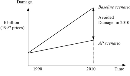
The measurement of benefits is essentially the measurement of avoided damages. Since the scenarios (other than Accession) generally simulate overall improvements in the environment, benefits will tend to get larger as we move from the baseline to the AP or TD scenarios. Where D refers to environmental damage, we estimate the benefits for the AP and TD scenarios in the following way:
DBASE - DAP = Benefits of AP DBASE -DTD = Benefits of TD
Figure 1.1 gives a stylised illustration of the benefit in 2010 of the AP scenario over baseline.
Damage Baseline scenario Avoided € billion Damage in 2010 (1997 prices) AP scenario 1990 2010 Time
Figure 1.1: Benefit of AP scenario in 2010
Benefits are defined in terms of individuals’ willingness to pay (WTP) to secure the benefits. Ideally a wider concept of benefits would include the macroeconomic benefits. Essentially, the difference between the WTP and macroeconomic benefits is one of scope. WTP tends to capture ‘partial’ benefits. These will approximate total benefits if the policy measures make only marginal changes to the economy. However, in terms of the scenarios adopted, the policy measures are not marginal, but involve fairly significant discrete changes. Thus, the wider concept of benefit is embraced allowing for the feedback effects of the policy on other prices and quantities in the economy.
This is possible only for those measures relating to the energy sector where the GEM-E3 model is used. In other cases, no macroeconomic model exists or the measures in question cannot easily be incorporated in such models (e.g. coastal waters, biodiversity etc).
Relevant WTP values for each environmental problems are drawn from an extensive literature review of the most recent and relevant monetary valuation studies conducted for this study. These give WTP estimates for environmental improvement or WTP estimates to avoid
environmental damage. Two main groups of monetary valuation techniques are used, stated and revealed preference techniques (for further details refer to Section 3 on monetary valuation techniques). Taking existing monetary valuation (WTP) studies and applying them outside of the site contexts where the study was originally carried out requires extensive use of ‘benefits transfer’ (see Section 4 on benefits transfer).
In order to calculate benefits in the future (i.e. in 2010), we assume that environmental quality has a rising relative price through time that is linked to growth in income per capita. The following formula is adopted to adjust the valuations accordingly:
WTP2010 = WTP1990. (Y2010/Y1990)e
Where WTP refers to willingness to pay valuations, Y is EU per capita GNP (assumed as:
Y2010 = € 19830 and Y1990 = € 14247, source RIVM) and e is the income elasticity of demand (assumed here as 0.3 refer to Section 5 on income elasticity of demand). An annual increase in relative prices for environmental quality of 0.5% per annum is arrived at1.
The likely time paths of benefits (and costs) are known in only a few cases, thus the benefit results are reported for a representative future year only, i.e. 2010. It is acknowledged that different time paths will produce potentially different results. When benefits are later compared with costs, the net benefits clearly depend on what is done, the scale of control measures and on the time paths of these measures. However, the research team is of the view that no major divergence of results will occur because of the choice of a representative year for benefits and costs.
Benefit estimates are summarised in Table 1.1 for those environmental problems with clearly defined AP / TD scenarios, such as climate change, acidification, tropospheric ozone, waste management, Human health, air quality and noise and nuclear risks. The values relate to benefits to the EU15 only unless otherwise stated. All values are benefits in 2010 only and are given in terms of € (1997 prices). For a more detailed discussion of the benefit estimates, refer to the benefits assessment for each environmental problem given in the Technical Reports.
1 Ideally, it should be decomposed by country since income per capita varies by country. However, we
RIVM report 481505020 - 9 –
Table 1.1 Summary of benefit estimates for each environmental problem Environmental problem Primary benefit
€ billion Secondary benefit € billion Climate change NT-AP FT-AP 3.7*3.7* 20.5 (11.5)13.4 (7.5) Acidification NT-AP FT-AP TD 21.7 (14.0) 25.2 (16.3) 58.9 (38.1) 7.1 (1.6) 7.8 (1.7) 12.6 (1.7) Tropospheric ozone NT-AP FT-AP TD 5.6 (0.7) 5.7 (0.7) 9.1 (1.2) -Waste management
AP with source reduction AP without source reduction TD max compost and recycle TD max incineration 8.7 7.2 10.3 -2.8 0.4 0.4 -Particulate matter AP TD 5.3 (3.1) (24.2 (14.0)) -Nuclear risks TD 6.8
-Where: ‘-’ = not available, NT = No Trade, FT = Full Trade, AP = Accelerated Policy scenario, TD = technology driven scenario. * benefit to world. Estimates given in brackets assume premature mortality is valued with VOLY, estimates not bracketed assume VOSL.
Note, primary benefits relate to the control of the pollutants, PX, causing the environmental problem X.
Primary benefits for climate change are due to the control of CO2, CH4 and N2O only. For acidification,
primary benefits are due to control of SOx, NOx and NH3, for tropospheric ozone primary benefit
estimates are due to the direct control of VOCs only and for Human health, air quality and noise, primary benefits relate to the end-of-pipe measures that reduce concentrations of primary PM10.
However, the control of PX pollutants can lead to the control of other pollutants Py causing other
environmental problems Y. This effect is known as the secondary benefit of measures to control X. The secondary benefits of climate change control are to acidification, low level ozone and Human health, air quality and noise (through the control of primary PM10 and secondary aerosols). Note that
the secondary benefits due to reductions of secondary aerosols are not estimated separately, they are already accounted for in the secondary benefits to acidification. The secondary benefits of acidification control are to tropospheric ozone and Human health, air quality and noise (i.e. through the control of primary PM10 and secondary aerosols). Note that the secondary benefits due to reductions in secondary
aerosols are subsumed in the primary benefit estimtes for acidification. The secondary benefits of waste management are to climate change control.
Uncertainty
Uncertainty is endemic to this study. The main sources of uncertainty in the benefit assessment approach are:
• scientific uncertainty about the impacts of given pressures on the state of the environment;
• economic uncertainty about the willingness to pay of the relevant population to avoid the impact;
Since these uncertainties are unavoidable the relevant approach is one which tries to estimate central tendencies and the confidence interval around that central tendency. Even though uncertainties at the various stages of the analysis may be multiplicative, estimates of central
tendency will tend to remain unchanged, although the dispersion about the mean will increase.
It is tempting to think that avoiding some of the stages of the analysis may reduce uncertainty. For example, monetary valuation (WTP) of premature mortality may be subject to confidence ranges which increases the range of uncertainty attached to the impact measure (e.g. lives lost). Casual commentators suggest that the monetary valuation stage should therefore be avoided. This is a mistaken strategy. First, the addition of the monetary valuation stage does not change the mean outcome. Second, the wider confidence interval that may emerge does indeed ‘increase’ the uncertainty of the estimate of effect, but if the monetary valuation stage is avoided other forms of uncertainty are added to the picture. Pursuing the pollution-health example, the analysis may be presented in terms of costs and lives prematurely lost, or it may be presented in terms of costs and the monetised (economic) value of lives prematurely lost. The former avoids the monetary valuation estimate; the latter explicitly includes it. But while the latter adds to uncertainty in the sense of increasing the confidence interval, the former increases other forms of uncertainty. Using the former, i.e. ‘lives lost prematurely’ assumes, for example, that all lives are to be equally weighted regardless of the length of life
expectancy lost, or the health state of those at risk etc. If this is not what is desired, then lives lost prematurely can be weighted by life expectancy and health state. But in so doing, the analyst superimposes a weighing on the indicator that has nothing to do with the perceptions or preferences of those at risk. In short, a new form of uncertainty is introduced, namely the uncertainty about the extent to which indicators are now responsive to individuals’ wants and desires, the basic value axiom of welfare economics.
Avoiding the monetary valuation stage also creates other forms of uncertainty. Where the impacts are measured in non-monetary units and compared to costs, there is no guideline on whether a policy is worth undertaking. Monetisation provides the guideline that policies should at least past a test to the effect that benefits should exceed costs. Cost-effectiveness indicators have no such test since it is never possible to tell whether an incremental unit of effectiveness is worth the cost of securing it. (Note also, that selecting any target of effectiveness, e.g. an upper limit on cost per life saved, automatically implies a monetary benefit estimate).
Avoiding the monetary valuation stage may seem like a rational response to the uncertainty embedded in the benefit estimates, but such a response adds at least two other forms of uncertainty. Firstly, the ‘democratic’ uncertainty, this is the extent to which any outcome is now responsive to individuals’ preferences, and secondly the ‘decision-making’ uncertainty, i.e. the extent to which rational trade-offs between costs and benefits can be made.
The reliability of the WTP values used in this study is tested, where possible, by using confidence intervals around the mean value. Table 1.1 reports mid values only, for ranges refer to the benefit estimates for each environmental problem given in the Technical Reports. The monetary valuation of premature mortality is a key area of uncertainty in this analysis. Where the probability of death is the same for all age groups in the population we adopt the value of a statistical life relevant to the general population, i.e. € 3.31 million (from € 2.6m 1990 prices converted to 1997 prices using the deflator 1.274). In those areas where deaths are mainly confined to the older age groups in the population we use a reduced VOSL, i.e. 70% of € 3.31 million = € 2.32 million.
For some environmental problems, fatalities occur over a long period, i.e. 1990-2010-2050 (i.e. nuclear risks) and thus the VOSL relevant to 1990 will not be relevant to the whole period. Rather, we would expect VOSL to rise as incomes rise. The effect of income growth is captured by introducing a rising relative price of risk aversion of 0.5% per annum, although there is limited information on the increase over time in the relative ‘price’ of risk. For further
RIVM report 481505020 - 11 –
information regarding the issue of premature mortality valuation see Section 6 on valuing statistical live.
Sensitivity
A number of assumptions are made for each separate benefit assessment. Some may have a significant effect on the results, while others will make only a minor difference. For purposes of transparency the key assumptions are stated clearly throughout. In order to see the effect on the net results if these assumptions are changed we conduct a sensitivity analysis. Thus, changes in the key assumptions and the associated quantitative effects are also reported.
RIVM report 481505020 - 13 –
2. POLICIES AND ENVIRONMENTAL PROBLEMS
Each environmental problem considered in this study contains a set of quantitative or qualitative ‘targets’ and each target corresponds to a scenario. Targets might be set in terms of given reductions in emissions, areas of land conserved for biodiversity etc. In order to inform the design of environmental policy, we need some idea of what policy instruments are best suited to the achievement of the targets.
The nature of policy instruments
A critical goal of policy towards the environment is cost-effectiveness: the achievement of the policy goal at least cost. In welfare economics terms, ‘least cost’ means least loss of economic wellbeing2. A narrower goal would be to measure costs solely in terms of the costs borne by the regulated agent in complying with the policy.
There are general reasons for supposing that economic instruments are best suited to achieving the least cost goal. Definitions of economic instruments (EIs) are not easy to provide. All forms of regulation impose a cost on the regulated agent, so that the presence of a financial incentive is not peculiar to economic instruments. It is widely argued that EIs leave the regulated agent with more flexibility on how to respond to policy. Thus, traditional ‘command and control’ (CAC) regulation might be regarded as setting target (what to achieve) and mechanism (how to achieve it), whereas EIs leave the regulated agent with the choice of what to achieve and how to achieve it, provided the overall policy goal is met in the aggregate. Thus, an individual regulated agent can emit pollution up to any level provided it pays the necessary environmental tax or holds the necessary permit to emit. The choice of the mix of abatement measures and tax payments/permit holdings is up to the regulated agent. But policy will have set an aggregate goal, for example a total level of emissions, that must be met and permits will be issued equal to this aggregate goal, or an estimate will have been made of the emission reduction effect of taxes so as to achieve the goal.
There are general reasons for supposing that EIs are best suited to achieving the least cost goal. However, the presumption that EIs are more cost effective than CAC is not always the case. In general, quite specific conditions have to be present for EIs to perform better than CAC3. These factors need to be taken into account in deciding the ‘match’ of policy instruments to
environmental problems.
Criteria for selecting policy instruments
Fundamental to this study is the use of ‘welfare economics’, it is therefore appropriate that the criteria for selecting ‘desirable’ policy instruments should be based on social cost benefit analysis. However, it is important to assess policy instruments against other considerations, such as distributional concerns (i.e. impacts to socio-economic class and region),
macroeconomic issues (competition and employment effects), administrative feasibility4 and subsidiarity (i.e. the ‘optimal jurisdiction’ issue, in other words, where policy is most effectively located). Subjecting policy instruments to many criteria for acceptability risks making almost all policy instruments fail. Similarly, we have no clear criteria (meta-criteria) for deciding which criteria are the most important. In order to identify rational policy instruments to meet AP scenario targets, we suggest that there are five groups of criteria for choosing a policy instrument, these are set out below:
2 Which, ideally, would be measured by the change in the sum of producers' and consumers' surpluses. In
practice, this measure will be available in only some cases.
3 See C.Russell, P.Powell and W Vaughan, Rethinking advice on environmental policy instrument choice in
developing countries, Paper to World Congress on Environmental Economics, Venice, June 1998.
4 Note that, 'political feasibility' is not explicitly considered, since the research team's concern is to define a
potential menu of policies. The extent to which such policies are politically feasible is not for the research team to judge.
• causal • efficiency • equity
• macro-economic • jurisdictional
The causal criterion answers the basic question: ‘does the policy instrument address the underlying economic failure’? If policy does not address the real causes of environmental degradation, it will have a high risk of failure. It is important to note that real causes do not equate with ‘pressures’ in the DPSR paradigm, nor what is popularly understood by ‘driving forces’. The underlying causes are i) market failures (i.e. not well defined property rights, missing markets and lack of information; ii) intervention failure (i.e. counter-effective subsidies and inconsistent policies; iii) implementation failures, i.e. if legislation exists, but is not fully implemented by Member States, iv) growth of real income, and v) population change, i.e. natural growth, migration and social change. Overall policy measures are targeted at the first three underlying causes only.
The economic efficiency criterion includes: i) benefit cost ratios, ii) cost-effectiveness, iii) benefits, and iv) public opinion for each policy instrument. The least-cost action is embodied in the cost-benefit approach and in cost effectiveness. Public opinion is included in efficiency because public opinion indicates public preferences, which in turn underlie the notion of willingness to pay. WTP is the building block of the benefits assessment.
The equity or distributional criterion considers: i) intra-generational equity (impacts to current socio-economic class, economic sector and region) and ii) inter-generational equity
(distributional impacts between generations).
The macro-economic criterion is mainly centred on the NTUA modelling of climate change policy. Policy instrument impacts considered are EU employment, GNP loss and competition effects. The macro-economic impacts are in the final report, see Chapter 4 Section 4.1, and for further details refer to Technical report on Socio-economic trends, macro-economic
impacts and cost interface.
The jurisdictional criterion concentrates on the issue of subsidiarity, i.e. where is policy most effectively located, such as, EU, national or local level. There are three main criteria upon which the level of subsidiarity can be assessed: i) gains from co-operation, ii) gains from harmonisation and co-operation and iii) gains in sustainable implementation.
Types of instruments
The list of instruments is potentially very large. Here we categorise them according to OECD classifications and the discussion in Panayotou (1998)5.
Command and control
• ambient based standards (e.g. µg of pollutant per m3);
• emission based standards (e.g. g of pollutant per km travelled in test conditions); • product based standards;
• technology based standards (BAT, BATNEEC), and • bans.
5 See OECD, Managing the Environment: the Role of Economic Instruments, OECD, Paris, 1994,
and T.Panayotou, Economic Instruments for Environmental Management and Sustainable Development, Earthscan, 1998, forthcoming.
RIVM report 481505020 - 15 –
Standards may be based on a per pollutant basis or on Integrated Pollution Control (IPC) considerations such that impacts on different environmental media are considered.
Economic instruments
Property rights
Property rights should be secure (enforceable) and transferable for economic efficiency to be assured. They will need to be attenuated in some form (ie certain uses will be forbidden) if they give rise to excessive externalities. Property rights can be private, communal or public, with a presumption that private and communal rights are to be preferred.
Fiscal instruments
• emission taxes (e.g. SOx charge); • effluent taxes (e.g. wastewater charge); • input taxes (e.g. pesticides or fertiliser tax); • (final) product taxes (e.g. packaging tax); • export taxes/import taxes;
• differential taxation (e.g. leaded/unleaded gasoline); • royalty (rent) taxation (e.g. forest taxation);
• land use taxes (taxes vary according to land use);
• accelerated depreciation (environmentally beneficial investments allowed to depreciate faster for tax offset purposes);
• subsidy removal (where subsidies harm the environment, e.g. CAP reform), and
• subsidies (where subsidies benefit the environment) (e.g. subsidies to renewable energy). Pollution taxes are formally equivalent to pollution charges so that no distinction between the two is made here. But charges and taxes otherwise differ: charges are for the use of a service, whereas taxes tend to raise revenue. The equivalence of charges and taxes in the pollution case arises because the polluter is using a public service - the assimilative capacity of the environment. In administrative terms the more important distinction is that taxes always form part of the fiscal structure and have therefore to be agreed by and administered by the tax authorities. Charges can be outside the control of tax authorities (inland revenue and customs).
Environmental charges
• user charges (e.g. entry fees to protected areas, road pricing);
• betterment charges (charges on properties which benefit from public infrastructure or environmental improvement), and
• impact charges (the obverse of betterment, ie charges on properties for making the environment worse, usually levied when property or land use changes).
Deposit - refund schemes and performance bonds
Here the charge is made in advance of any damage occurring, and refunds are given when the product is safely disposed of or recycled or the environmental degradation is made good. Bonds act in the same way: the bond has to be purchased at the onset on economic activity (e.g. quarrying) and can only be redeemed when there is an indication that restoration has occurred. • deposit-refund (tax-subsidy) schemes (e.g. on returnable bottles and cans);
• environmental performance bond (e.g. mining, quarrying, forest logging, waste arisings), and
• accident bonds (e.g. for oil spills).
Liability systems
Liability systems rest on the threat of legal action in the event of non-compliance. The charge is collected only in the event of damage occurring and liability systems thus have similarities with
bonds (above). However, bonds collect the charge early on and refund it later. Liability systems collect the charge only in the event of damage.
• legal liability (is ‘strict’ when libaility exists regardless of precautions taken, and is ‘negligence’ when actions taken to avoid damage are taken into account);
• non-compliance fines (charges at some penal rate for emissions above standards);
• joint and several liability (any one contributor to damage can be held responsible for all damage), and
• liability insurance (insurance market premia in the event of damage in a liability context).
Financial incentives
Financial incentives involve the creation of funds used for environmental improvement. Funds may come directly from government grants, from specific taxes or from external ‘deals’ such as a debt-for-nature swap, Global Environment Facility incremental cost financing etc. Financial incentives are especially important for the Economies in Transition.
Tradable quotas and offsets
Tradable quotas can relate to emissions (tradable emission permits) or resources (tradable resource quotas). Offsets relate to bargains between several parties such that an emission reduction obligation in one location is offset by reducing emissions in another location. The credits may not be traded (joint implementation) or they may be traded (tradable emission credits).
• joint implementation (mainly CO2 but not exclusively);
• tradable emission permits (SOx in the USA, and limited use in Europe): auctioned / grandfathered;
• tradable water rights;
• tradable fishing quotas: auctioned / grandfathered, and
• tradable development rights (land is zoned, some of it for development and rights to that development then become tradable).
Voluntary agreements
Voluntary agreements involve an understanding, sometimes backed by legal requirements, between government and industry such that industry ‘self regulates’. Self regulation involves setting agreed environmental targets, leaving industry to determine its own means of achieving those targets, such to some overall broad agreement on mechanisms.
Information
Two forms of information provision are considered:
• labelling (labelling of environmental performance, resource content etc) • disclosure (publication of pollution profile of companies etc)
Matching policies to environmental problems
The following matrices ‘match’ environmental problems and economic instruments based on the five criteria indicated above. The allocation is necessarily judgmental but conforms with exercises elsewhere that have attempted to link instruments and problems in various different contexts. Environmental funds are excluded from the analysis because they can be created through the other instruments. However, externally financed funds are of importance to ‘economies in transition. Property rights are also excluded as they are of less concern in Europe. Nonetheless, each environmental problem is prefaced with a remark about property rights. These matrices are the foundations for the policy packages / assessments for each environmental issue presented in this Annex.
RIVM report 481505020 - 17 –
Stratospheric ozone depletion
Property rights in the ozone layer were established by the Montreal Protocol and the subsequent amendments and agreements. Rights are held by all signatory countries. Policy measures relate to controls on domestic production and controls on imports due to the fact that imported ODSs contribute to domestic consumption totals which, are the subject of ‘caps’. Imports of recycled ODSs do not count against domestic consumption. Financial incentives (not shown here) relate to the Multilateral Fund which finances phase-out in the developing countries. Note also that the Montreal Protocol makes extensive use of restrictions on international trade in CFCs.
Stratospheric ozone depletion Issue: reduce emissions of ODSs Initiatives
Fiscal incentives CFC taxes exist in USA
Import duty reductions for ODS
Charges
-Deposit refund schemes and performance bonds DRS for recycled ODSs
Liability
-Tradable permits Reduction in trading in USA
Permit trading for import allowances Voluntary agreements VAs to restrict imports
Information Labelling products
Climate change
Property rights established by FCCC, 1992 and Kyoto Protocol 1997/8. Financing for LDC emissions reduction takes place via incremental cost financing from the Global Environment Facility, and through joint implementation schemes. The Clean Development Mechanism introduced in the Kyoto Protocol could evolve into a North-South JI scheme. JI East-West is enabled under the Kyoto Protocol.
Climate change
Issue reduce emissions of GHGs and sequestering carbon Initiatives
Fiscal incentives Carbon / energy taxes in place in several countries;
Excise duties; Aviation tax; Methane tax;
Charges
-Deposit refund schemes and performance bonds
-Liability
-Tradable permits Joint implementation in place: over 200 deals Tradable efficiency permits for car manufacturers Voluntary agreements Carbon neutral pricing schemes
Voluntary offset schemes
Information Energy conservation campaign
Emission disclosure
Major accidents
Major accidents occurring in a single Member State and not affecting other States need to be distinguished from accidents with potential transboundary effects. Nuclear, oil sill and chemical risks can easily be transboundary, suggesting that preventive and emergency response measures should be co-ordinated at EU level. To be realistic, such measures need to incorporate funds, akin to the Montreal Protocol Multilateral Fund, to finance risk reduction in the EITs. Such a
fund exists for nuclear accidents (EU, Canada and US financed) and there are emergency response communications co-ordinated across Europe.
Major accidents
Issues reducing high risk nuclear reactors, reducing chance and impact of chemical disasters Initiatives
Fiscal incentives Tax on energy output
Tax on port calls Output tax
All to fund emergency responses
Charges
-Deposit refund schemes and performance bonds Could introduce performance bonds in EU
Liability Negligence liability in EU
Tradable permits
-Voluntary agreements
-Information
-Biodiversity loss
Unless privately owned or legally protected, most biodiversity is not the subject of property rights. Ownership of land by conservation groups or the state can contribute substantially to reducing biodiversity loss. Effectively, a market in biodiversity is created, although the medium is the land and property market itself. In other cases, market creation may be direct, e.g. by commercialising products from wild species, creating an incentive to conserve the species for profit. Since pollution is a cause of biodiversity loss it should be noted that all pollution reduction measures (see other environmental problems) will have an impact on biodiversity.
Biodiversity loss
Issue: reducing biodiversity loss through reduced habitat loss Initiatives
Fiscal incentives Agri-environmental schemes; environmentally sensitive areas, country side access schemes, country side stewardship schemes, Arable stewardship schemes, habitat schemes, moorland schemes, organic farming schemes, nitrate sensitive areas,
Payments for set-aside; Outright land purchases;
Tax allowances on money and land donations to conservation;
Tax allowances on reforesting, soil and water conservation, and
Easements and purchase of development rights;
Charges Park entrance fees, user permits with earmaked
revenues;
Fines for damage to natural assets. Deposit refund schemes and performance bonds Land restoration with performance bonds
Liability Liability for pollution damage
Tradable permits Offset requirements, e.g. loss of wetland has to be offset by creation of new wetlands, i.e. mitigation banking;
Tradable development rights; Tradable fishing quotas.
Voluntary agreements Voluntary management agreements: Sweden, Austria, UK.
RIVM report 481505020 - 19 –
Acidification and eutrophcation
Property rights to transboundary pollution reduction have been established by the Convention on Long Range Transport of Air Pollution in Europe and by various EU legislation.
Acidification and eutrophication
Issue: reducing emissions of SOx, NOx and NH3
Initiatives
Fiscal incentives S and N taxes
NH3 tax with mineral accounting, or livestock tax
Charges
-Deposit refund schemes and performance bonds
-Liability
-Tradable permits Possible tradable permits in SOx and NOx
Voluntary agreements
-Information
-Chemical risks
Chemical risks
Issue: reducing risks from heavy metals, pesticides and POPs Initiatives
Fiscal incentives Pesticide tax
Battery charges Chemicals charges
Charges
-Deposit refund schemes and performance bonds Application to hazardous products, e.g. batteries
Liability
-Tradable permits Lead trading
Voluntary agreements VAs possible
Information Ecolabelling
Water management
Water management
Issue: improving water availability through management of supply and demand, and improving quality of ground water and surface water.
Initiatives
Fiscal incentives Pesticide tax
Fertiliser tax
Charges Abstraction charges
Effluent charges Deposit refund schemes and performance bonds
-Liability
-Tradable permits Tradable water rights
Tradable effluent rights
Tradable quotas for pesticides and fertilisers
Voluntary agreements
-Information
Waste management
Waste management
Issue: reducing waste at source, increase recyling and re-use, minimise landfill Initiatives
Fiscal incentives Recycling credits;
Virgin materials tax; Landfill tax; Incinertion tax.
Charges Collection charges
Deposit refund schemes and performance bonds DRSs for returnable containers; DRSs for batteries.
Liability
-Tradable permits Tradable recycling quotas
Voluntary agreements Producer responsibility agreements
Information
-Tropospheric ozone
Many of the policies suitable for acidification will also have a significant impact on the problem of tropospheric ozone.
Tropospheric ozone
Issue: reduce NOx and VOC emissions (i.e. the precursors to low level ozone)
Initiatives
Fiscal incentives N tax
VOC tax
Charges
-Deposit refund schemes and performance bonds
-Liability
-Tradable permits Tradable quotas in VOCs and NOx
Voluntary agreements
-Information Eco-labelling for solvents
Coastal zone management
See also climate change, biodiversity loss and chemical risks. Coastal zone management
Issue: reduce coastal erosion (see climate change), reduce habitats damage (see biodiversity loss), improve bathing water quality.
Initiatives
Fiscal incentives for:
Bathing water quality Tax non compliance with Bathing Water Directive
Charges Possible beach charges
Deposit refund schemes and performance bonds
-Liability Owner liability for failure to meet Bathing Water Directive;
Owner liability and performance bonds against oil spills.
Tradable permits Transferable development rights;
Tradable quotas for fishing
Voluntary agreements
-RIVM report 481505020 - 21 –
Human health, air quality and noise Human health, air quality and noise
Issue: reduce exposure to noise, reduce urban pollutants especially PM10, PM2.5. Initiatives
Fiscal incentives Air pollution taxes: see acidification Noise taxes for vehicles
Airport landing charges varied with noise levels;
Charges Road user charges according to noise levels and
congestion, Deposit refund schemes and performance bonds
-Liability
-Tradable permits Tradable efficiency permits for car manufacturers
Voluntary agreements
-Information
-Soil degradation
Soil degradation
Issue: reduce soil degradation from all causes but especially from water erosion Initiatives
Fiscal incentives Tax offsite damages
Subsidies to good practice
Charges
-Deposit refund schemes and performance bonds
-Liability
-Tradable permits
-Voluntary agreements Management agreements
Information Extension services
Structure for policy packages
A policy package paper exists for each environmental problem. The structure of the policy packages is based on the following format:
1. Key issues associated with each environmental problem are described. This may include
a comment about the expected benefits from environmental control as well as the most suited policies based on the five criteria;
2. Available instruments: based on the matrices that ‘match’ policies to environmental
problems presented above and guided by the results of the ‘policy assessment’, the policy packages give more detail to the recommend policies. The section also provides
experience with policy instruments in the EU15 (and elsewhere if relevant) and where
possible an indication of the effectiveness of the policy instruments is given, i.e. a summary of what is known about the effectiveness of actual instruments, including simulations of hypothetical instruments and judgements.
Structure of policy assessments
This section assesses the suggested policies against the five criteria described above, i.e. i) causal criterion,
ii) efficiency criterion, iii) administrative complexity, iv) equity criterion, and v) jurisdictional criterion.
RIVM report 481505020 - 23 –
3. MONETARY VALUATION TECHNIQUES
Introduction
The economic approach to valuing environmental changes is based on people’s preferences for changes in the state of their environment. Environmental resources typically provide goods and services for which there are either no apparent markets or very imperfect markets, but which nevertheless can be important influences on people’s well-being. Examples include the quality of air, which affects people’s health, crop yields, damage to buildings, and acidification of forests and fresh waters.
However, the lack of markets for these services means that unlike man-made products, they are not priced, therefore their monetary values to people cannot be readily observed. The underlying principle for economic valuation of environmental resources, just as for man-made products, is that people’s willingness to pay (WTP) for an environmental benefit, or conversely, their willingness to accept compensation (WTA) for environmental degradation, is the appropriate basis for valuation.
If these quantities can be measured, then economic valuation allows environmental impacts to be compared on the same basis as financial costs and benefits of the different scenarios for environmental pollution control. This then permits an evaluation of the net social costs and benefits of each scenario for the different environmental issue.
The lack of markets and prices for many environmental goods and services means that the challenge for economists is twofold. The first task is to identify the ways in which an environmental change affects well-being; this is addressed in the next section, where the components of ‘total economic value’ of a resource are explained. The second task is to
estimate the value of these changes through a variety of direct and indirect valuation
techniques, exposition of which is given in the following sections.
Total Economic Value
The monetary measure of the change in society’s well-being due to a change in environmental assets or quality is called the total economic value (TEV) of the change. To account for the fact that a given environmental resource provides a variety of services to society, TEV can be disaggregated to consider the effects of changes on all aspects of well-being influenced by the existence of the resource.
TEV can be divided into use values and non-use values, the latter also being called ‘passive use values’. Use values include:
• direct use values, where individuals make actual use of a resource for either commercial purposes (e.g. harvesting timber from a forest) or recreation (e.g. -swimming in a lake)
• indirect use values, where society benefits from ecosystem functions (for example, watershed protection or carbon sequestration by forests)
• option values, where individuals are willing to pay for the option of using a resource in the future (for example, future visits to a wilderness area)
Non-use values can take the form of:
• existence values, which reflect the fact that people value resources for ‘moral’ or ‘altruistic’ reasons, unrelated to current or future use
• bequest values, which measure people’s willingness to pay to ensure their heirs will be able to use a resource in the future
To arrive at an estimate of the net change in societal well-being arising from an environmental change, we must consider each of these elements in turn. The total economic value (TEV) of a change is the sum of both use and non-use values:
TEV = use values + non-use values
= direct use + indirect use + option + existence + bequest values
Table 2.1 presents a taxonomy for environmental resource valuation, using the total economic value of a forest as an illustration.
Table 2.1 Economic taxonomy for environmental resource valuation Total Economic Value
Use Values Non-use Values
Direct Use Indirect Use Option Value Bequest Value Existence Value Outputs
directly consumable
Functional
benefits Future direct andindirect values Use and non-usevalue of environmental legacy value from knowledge of continued existence • food • biomass • recreation • health • flood control • storm protection • nutrient cycles • biodiversity • conserved habitats • habitats • prevention of irreversible change • habitats • species • genetic • ecosystem The first step in estimating any of these values is the definition and measurement of the environmental problem. This often includes an element of scientific uncertainty that can, at times, be quite significant. The accuracy of economic valuation is therefore dependent on accurate scientific identification and quantification of the environmental change in order to estimate people’s preferences for or against it.
Valuation Techniques
The practical problem with economic valuation is one of deriving credible estimates of people’s values in contexts where there are either no apparent markets, or very imperfect markets. In the case of marketed goods, price is the measure of willingness to pay and can be readily observed. However, in the case of non-marketed goods and services we need to elicit this value in different ways. There are two broad approaches to valuation, each comprising several different techniques, as illustrated in Figure 2.1.
• Revealed preference techniques, which infer preferences from actual, observed, market-based information. Preferences for environmental goods are revealed indirectly when individuals purchase marketed goods which are related to the environmental good in some way.
• Stated preference techniques, which attempt to elicit preferences directly by use of questionnaire, such as contingent valuation. All valuation of non-use values depends on these techniques.
We consider each of these approaches in turn, highlighting when each could be used, their advantages and drawbacks and their applicability to waste management problems.
T
ot
al
E
conom
ic
V
al
ue
Use
V
al
ue
R
evea
led P
ref
er
enc
es
co
nven
tion
al an
d sur
roga
te ma
rke
ts
No
n-us
e V
al
ue
Sta
ted Pr
ef
er
enc
es
hy
pot
het
ical
ma
rk
et
s
ra
nd
om
ut
ili
ty
/
di
sc
re
te
ch
oi
ce
m
ode
ls
(W
T
P
)
tra
vel
co
st
me
th
o
d
(W
T
P
)
av
er
tin
g
b
eh
avio
ur
(W
T
P
)
ma
rk
et
pri
ces
(W
T
P
)
co
n
tin
g
en
t
va
lu
at
io
n
(W
T
P/W
TA
)
co
nj
oi
nt
an
al
ys
is
(W
T
P/W
TA
)
he
don
ic
pr
ic
in
g
la
bo
ur
ma
rk
et
(W
T
A
)
pro
per
ty
ma
rk
et
(W
T
P
)
be
ne
fits t
ra
ns
fer
d
ose
r
esp
on
se
/
pr
od
uc
ti
on
fu
n
ctio
ns
ch
oi
ce
ex
peri
m
en
ts
pa
ir
ed
com
pa
riso
ns
cont
in
ge
nt
ra
nk
in
g
cont
inge
nt
/
co
nj
oi
n
t ratin
g
F
ig
ur
e
2.
1: A t
ypol
og
y
of
m
on
eta
ry
val
uat
io
n
met
hod
s
markets in which environmental factors have an influence. For example, there are markets for certain goods to which environmental commodities are related, as either substitutes or complements to the goods in question. In this way people’s actions in actual markets reflect, to a certain extent, their preferences for environmental assets.
There are four main revealed preference techniques that are considered in the sections that follow.
1. Averting behaviour
2. Hedonic pricing (of property and labour) 3. Travel cost method
4. Random utility and discrete choice modelling
Averting Behaviour
The basis for the averting behaviour technique is the observation that marketed goods can act as substitutes for environmental goods in certain circumstances. When a decline in environmental quality occurs, expenditures can be made to mitigate the effects and protect the household from welfare reductions. For instance, expenditure on sound insulation can indicate households’ valuation of noise reduction; expenditure on household water filters can be used to estimate economic values of clean water.
The method is applicable in situations where households spend money to offset environmental impacts. It requires data on the environmental change and its associated substitution effects. Fairly crude approximations can be found by simply looking directly at changes in expenditures on the substitute good resulting from some environmental change. Advantages of these models are that they have relatively modest data requirements and can provide theoretically sound estimates based on actual expenditures. However, they can give incorrect estimates if other important aspects of individuals’ behavioural responses are ignored. For example, individuals may engage in more than one form of averting behaviour in response to any one environmental change. Additionally, the averting behaviour may have other beneficial effects that are not considered explicitly, for example sound insulation may also reduce heat loss from a home. Furthermore, averting behaviour is often not a continuous decision but a discrete one: for example, a smoke alarm is either purchased or not. In this case the technique will tend to underestimate the value of the environmental good.
Hedonic Pricing
This technique depends on analysis of existing markets where environmental factors have an influence on price. The example most frequently used is that of the housing market, as the environmental attributes of a property will vary according to its location. For example, noise levels will be higher close to an airport and, other characteristics being equal, this can be expected to lower the price of a property in the area. Similarly, two identical properties which differ only in, say, the local air quality, will differ in value to the extent that people find one air quality preferable to the other. The difference can be viewed as the value attached to the difference in air quality as measured by willingness to pay (WTP).
The hedonic property price (HPP) method can be used even when properties differ in many factors other than environmental quality provided that data are detailed enough. With the use of appropriate statistical techniques, the hedonic approach attempts to (i) identify how much
RIVM report 481505020 - 27 –
of a price differential is due to a particular environmental difference between properties, and (ii) infer how much people are willing to pay for an improvement in environmental quality that they face and what the social value of the improvement is. The same technique has also been applied to labour in the valuation of work-related risk in hedonic wage (HW) studies. Identification of wage differentials due to differences in safety risks, for example, will give an indication of willingness to accept compensation (WTA) for incurring these risks, which can be used as a measure of the benefits of improving safety.
This technique can in theory be used to estimate factors such as the disamenity costs of location near to landfill sites, or air quality near to incinerators.
Travel Cost Method
Many natural resources are used extensively for the purpose of recreation. It is often difficult, however, to value these resources because no prices generally exist for them. The travel cost approach is based on the fact that, in many cases, a trip to a recreational site requires an individual to incur costs in terms of travel, entry fees, on-site expenditures and time. These costs of consuming the services of the environmental asset are used as a proxy for the value of the recreation site and changes in its quality.
Clearly, because travel cost models are concerned with active participation they measure only the use value associated with any recreation site. The method is now well -established as a technique for valuing the non-market benefits of outdoor recreation resources. It is useful because it is based on actual observed behaviour. However, the technical and data requirements are such that it is not readily applicable.
Random Utility or Discrete Choice Models
While the travel cost method is useful for measuring total demand or WTP for a recreational site, this technique is less useful for estimating the value of particular features or assets of the site which may be of interest. Random utility models have been developed for this purpose. The emphasis of random utility or ‘discrete choice’ models is on explaining the choice between two or more goods with varying environmental attributes as a function of their characteristics. This can be useful where, for example, polluting activity causes damage to some features of a recreational site but leaves others relatively unharmed.
This can be illustrated using a simple example from a choice of transport mode. Supposing that, when undertaking a given journey, an individual faces the choice of travelling by taxi or by public transport. A taxi will take 20 minutes and cost €5, whereas public transport will take an hour but cost € 2. If the individual chooses to travel by taxi, it can be inferred that s/he judges the difference of 40 minutes in time to be worth at least the € 3 difference in fare. In other words, the value of the individual’s time is at least €4.50 per hour.
Another example is the choice between bottled water and tap water for drinking. The former is more expensive but associated with better quality. Therefore, the price difference between bottled and tap water is an indication of the value of risk in this context.
Replacement Cost
The replacement cost technique uses the cost of replacing or restoring a damaged asset to its original state as the measure of the benefit of restoration. The approach is widely used, largely because it is comparatively easy to apply.
This approach is valid where it is possible to argue that the remedial work must take place because of some other constraint such as an environmental standard. Replacement will only be efficient, however, if the environmental standard itself is economically efficient. Otherwise
the approach estimates only the costs of replacement: it is not a technique for benefit estimation. Indeed, if costs of replacement are used to estimate the benefits of replacement, then a benefit-cost ratio of one will always result, and a replacement project will always appear justified.
Information on replacement costs can be obtained from direct observation of actual expenditure on restoring damaged assets or from engineering estimates of restoration costs. The technique implies various assumptions, for instance, that complete replacement is, in fact, feasible. In general, however, the potential for confusion between costs and benefits means that the replacement cost technique needs to be applied with some care.
Stated Preference Techniques
Stated preference techniques enable economic values to be estimated for a wide range of commodities which are not traded in markets. In addition, these techniques are the only way to estimate non-use value of environmental resources. Here, we consider two approaches:
1. Contingent valuation 2. Conjoint analysis
Contingent Valuation
In contingent valuation (CV) studies, people are asked directly to state what they are willing to pay for a benefit or to avoid a cost, or, conversely, what they are willing to accept to forego a benefit or tolerate a cost. A contingent market defines the good itself, the institutional context in which it would be provided, and the way it would be financed. The situation the respondent is asked to value is hypothetical (hence, ‘contingent’) although respondents are assumed to behave as though they were in a real market. Structured questions and various forms of ‘bidding game’ can be devised to assess the maximum willingness to pay. Econometric techniques are then applied to the survey results to derive the average bid value, i.e. the average WTP.
There are three basic parts to most CV surveys. First, a hypothetical description of the terms under which the good or service is to be offered is presented to the respondent. Information is provided on the quality and reliability of provision, timing and logistics, and the method of payment. Second, the respondent is asked questions to determine how much s/he would value a good or service if confronted with the opportunity to obtain it under the specified terms and conditions. These questions take the form of asking how much an individual is willing to pay for some change in provision. Respondents are reminded of the need to make compensating adjustments in other types of expenditure to accommodate this additional financial transaction. Econometric models are then used to infer WTP for or WTA the change. Finally, questions about the socio-economic and demographic characteristics of the respondent are asked in order to relate the answers respondents give to the valuation question to other characteristics of the respondent, and to those of the policy-relevant population.
CV is likely to be most reliable for valuing environmental gains, particularly when familiar goods are considered, such as local recreational amenities. While the accuracy of results also depends on careful construction of the survey, a set of guidelines for applying CV to derive reliable estimates of non-use values is developed by the US National Oceanic and Atmospheric Administration (NOAA) panel (Arrow et al.,, 1993). This is now being extended to cover all CV studies.
RIVM report 481505020 - 29 –
Conjoint Analysis
Conjoint analysis (CA) is a broad term used to cover several different techniques, all of which are survey methods, but they involve asking individuals to rank alternatives rather than explicitly express a WTP or WTA. For contingent ranking, the inclusion of prices in some of the alternatives enables rankings to be converted to monetary values. Other aspects are similar to contingent valuation.
Again, the main application of relevance to the current study has been in the context of human health and landscape effects, as well as disamenity.
Dose- and Exposure-Response Functions
Dose-response functions (DRFs) measure the relationship between a unit concentration of a pollutant and its impact on the relevant receptor. Exposure-response functions (ERFs) are based on the same principle but measure the response with respect to the exposure. Exposure is a measure of the levels of a pollutant in the environment surrounding the receptor in question. For example, a person may be exposed to a certain concentration of an atmospheric pollutant, but the dose received will depend on the amount inhaled, which is higher during exercise and lower during rest. In general, effects will be more closely related to dose, but it is much easier to measure exposure. Hence it is important to recognise that any dose-response function is often represented by the approximation of an exposure-response function (ApSimon et. Al., 1997).
Dose-response techniques are used extensively where a physical relationship between some cause of damage, such as pollution, and an environmental impact or ‘response’ is known and can be measured. Once the relationship has been estimated, then WTP measures derived from either conventional market prices (which are adjusted if markets are not efficient) or revealed/inferred prices (where no markets exist) using one of the techniques described in the previous section. The physical damage is multiplied by this shadow price, or value per unit of physical damage, to give a ‘monetary damage function’.
The approach is theoretically sound, and can be used wherever the physical and ecological relationships between a pollutant and its output or impact are known. The specification of the D/ERF is crucial to the accuracy of this technique, and is the main source of uncertainty. Difficulties and uncertainties may arise in: identifying the pollutant responsible for the damage and all possible variables affected; isolating the effects of different causes to determine the impact on a receptor, e.g. synergistic effects where several pollutants or sources exist; identification of damage threshold levels and the long term effects of low to medium levels of pollution. All these problems make it difficult to determine the appropriate empirical specification of the functional form. Additionally, there is the further complication that evidence of a physical response may not be economically relevant if individuals are not concerned about it and, therefore, do not attach a value to avoiding it. For these reasons, large quantities of data may be required and the approach may be costly to undertake.
If, however, the D/ERFs already exist and the impacts are marginal, the method can be very inexpensive and provide reasonable first approximations to the true economic value measures.
RIVM report 481505020 - 31 –
4. BENEFITS TRANSFER
The benefit assessment procedure conducted in this study makes extensive use of ‘benefits transfer’, i.e. taking existing monetary valuation (willingness to pay) studies and applying them outside of the site contexts where the study was originally carried out. There is in fact no alternative to this procedure if any use at all is to be made of benefit valuation techniques. The approach implicitly underlies the procedures used, for example, by ExternE, although, as it happens, their use of transferred functions may be more basic than ours in at least one respect. They choose specific functions and apply these across Europe. In our case we make some attempt to engage in ‘meta studies’ where that is possible. Technically, the alternative is to carry out willingness to pay studies across all EU15 countries for all environmental problems. Clearly, this is not possible. Nonetheless, we should be aware that the procedure involves risks and errors. This note serves to set out the nature and problems involved in benefits transfer. It should be noted that the literature analysing the validity of transfer techniques is very small.
(a) Transferring average WTP from a single study to another site which has no study
The basic idea is to ‘borrow’ an estimate of WTP in context i and apply it to context j, but making adjustments for the different features of the two contexts. For example, if incomes vary we might have
WTPj = WTPi(Yj/Yi)e
where Y is income per capita, WTP is willingness to pay, and ‘e’ is the income elasticity of demand, i is usually called the study site and j the policy site.
A typical example of such an approach is given by Krupnick et al., (1996) who transfer US WTP for various health states to Eastern Europe using the ratio of wages in the two areas and an income elasticity of demand of 0.035. The significance of the procedure can be realised since the wage ratio raised to e=0.035 produces a WTP in Eastern Europe equal to only 8% of that in the USA.
A second, common adjustment is for population size and, less frequently, for the distribution of population characteristics, e.g. age.
Note that the transfer is ‘assumed’ to be correct: no separate validation is carried out. This is similar to most of the transfer of values used in the EU Priorities study.
(b) Testing the equality of means at two sites where studies exist
Where there are two sites both with actual WTP estimates we can obtain some idea of the validity of benefits transfers by comparing the two mean WTPs. We wish to know if they are statistically the same. If they are, then there is some reason to feel confident that the results from a given site can be transferred to another site, as in (a) above.
Where the underlying distribution of WTP is thought to be normal, parametric tests can be used (eg t-tests) to determine if the mean WTP results at the two (or more) sites are statistically the same. Where this restriction is thought to be unreasonable, then non-parametric tests are required. More sophisticated testing can be done, e.g. to find out if the two underlying WTP distribution (not just the means) are statistically the same.
(c) Transferring benefit functions
A more sophisticated approach is to transfer the benefit function from i and apply it to j. Thus if we know that WTPi = F(A, B, C, Y) where A,B,C are factors affecting WTP at site i, then we can estimate WTPj using the coefficients from this equation but using the values of A, B, C, Y at site j.
Alternatively, we can use meta analysis to take the results from a number of studies and analyse them in such a way that the variations in WTP found in those studies can be explained. This should enable better transfer of values since we can find out what WTP depends on. Whole functions are transferred rather than average values, but the functions do not come from the single site i, but from a collections of studies.
(d) Is transferring functions valid?
How do we know if transferring functions is a valid procedure? As with the procedure under (a), we have no direct test that the result is ‘correct’. The literature has proceeded by taking estimated demand functions at site i and site j and then comparing them to see if, statistically, they are the same. This involves at least testing for the equivalence of the coefficients in the two functions, e.g.
WTPi = x + a1 A + b1 B + c1 C and WTPj = x + a2 A + b2 B + c2 C
so that we require a1 = a2 etc, where equality here is statistical equality (Loomis, 1992).
Recent literature has suggested that even if it is valid to transfer benefit functions, based on statistical equality of coefficients, the resulting estimates of benefits may be in error. This is because benefits may not be a linear function of the coefficients. Downing and Ozuna (1996) take demand functions for 8 sites in Texas and conclude that around 50% of functions are transferable (have the same coefficients) but that only a small minority would yield reliable benefit estimates. This has led Bergland et al., (1995) to suggest that both valuation functions and benefits estimates must be transferable (see the ‘protocol’ below.. )
Generally, the literature testifies to the unreliability of transferring benefit functions (Loomis, 1992; Downing and Ozuna, 1996; Bergland et al.,, 1995; Parsons and Kealy, 1994). Most studies seem to suggest that transferring functions is better than transferring average values, but that both are subject to significant margins of error (Kirchhoff et al.,, 1997).
(e) Validating benefits transfer
The test in (d) above involves taking actual demand functions and seeing whether they are statistically the same and will produce similar benefit estimates. Another test would be to take a WTP estimate from i and apply it to j using a simple procedure such as the one set out in (a) above. Then, a full WTP study would be carried out in j and the mean WTP result would be compared with the ‘transferred’ WTP.
Navrud (1997) has done this for minor impaired health states to see if WTP estimates from the USA can be transferred to Europe (in fact, to Norway). He concludes that the transferred estimates significantly overstate the ‘actual’ WTP as derived from a contingent valuation study in Norway.