Is the amount of pesticides in Dutch regional surface waters correlated with toxic effects?

(1)

Is the amount of pesticides in Dutch regional surface waters correlated with toxic effects? P. van Beelen, M. Wouterse, J.J. Bogte, D. de Zwart, B. van Dijk, J.L. Maas*, A. Espeldoorn*, and A.C. de Groot

*_{Dutch National Institute of Inland Water Management and Waste Water Treatment (RIZA).}

This investigation has been performed by order and for the account of the Directorate General for

Environmental Protection, Directorate for Soil, Water and Rural Environment within the framework of project 860701/01/PT, Toxic Pressure measurements.

(2)

Samenvatting

In de zomer van 2002 werden Nederlandse regionale oppervlaktewateren bemonsterd voor de analyse van 53 bestrijdingsmiddelen en voor toxiciteitsexperimenten. De hydrofobe

chemicaliën (inclusief de meeste bestrijdingsmiddelen) werden geconcentreerd door sorptie aan kunsthars voorafgaand aan de toxiciteitsexperimenten. The concentraten werden getest met behulp van de PAM test met de groenalg Selenastrum capricornutum, de MicroTox test met de bacterie Vibrio fisheri, the IQ test met de watervlo Daphnia magna, een test met de kreeftachtige Thamnocephalus platyurus en een test met de rotifeer Brachionus calyciflorus. Om 50% inhibitie te veroorzaken moesten de monsters meer dan 100 keer geconcentreerd worden voor de rotifeer test en meer dan 10 keer voor de andere testen. In 44 van de 45 monsters was de concentratie van de gemeten bestrijdingsmiddelen te laag om de toxiciteit te verklaren. Dit impliceert dat de bijdrage van deze bestrijdingsmiddelen aan de totale toxiciteit vermoedelijk erg laag is in de meeste monsters, met uitzondering van één monster dat 3,1 µg parathion /liter bevatte. Dit is dichtbij de parathion concentratie die, volgens de

wetenschappelijke literatuur, de mobiliteit van Daphnia magna met 50% vermindert. In onze toxiciteitsexperimenten moest het monster wel 20 keer geconcentreerd worden om 50% van Daphnia magna te remmen. Op dit moment hebben we nog geen goede verklaring voor deze discrepantie. De standaard Daphnia magna test zou kunnen verschillen van de hier gebruikte Daphnia IQ test. Verder onderzoek is nodig om te bepalen of bestrijdingsmiddelen werkelijk een acuut risico vormen voor aquatische ecosystemen in Nederlandse regionale

(4)

Summary

In the summer of 2002, Dutch regional surface waters were sampled for analysis of 53 different pesticides and for toxicity measurements. The hydrophobic chemicals, including many pesticides, were concentrated by sorption to synthetic resins before the toxicity measurements. The concentrates were tested with the PAM test using the green algae

Selenastrum capricornutum, the Microtox test using the bacterium Vibrio fisheri, the IQ test using the water flea Daphnia magna, a crustacean test using Thamnocephalus platyurus and a rotifer test using Brachionus calyciflorus. In order to obtain 50% inhibition, the samples had to be concentrated over 100 times for the rotifer test and over 10 times for the other tests. In 44 out of 45 samples the observed toxicity was too high to be explained by the low

concentrations of the measured pesticides. This implies that the contribution of these pesticides to the total toxicity is probably very low in most samples, except for one sample that contained 3.1 µg/liter of parathion. This is close to the parathion concentration that, according to the scientific literature, can reduce the mobility of Daphnia magna for 50%. In our toxicity tests however, this sample had to be concentrated 20 times in order to inhibit 50% of the Daphnia magna. At the moment, we do not have a good explanation for this

discrepancy. The standard Daphnia magna test might differ from the rapid Daphnia IQ test performed here. Further research is needed to determine whether pesticides can really pose an acute threat for aquatic ecosystems in Dutch regional surface waters.

(5)

1. Introduction

In the low parts of the Netherlands most of the rainwater flows via small ditches and larger waterways to a pumping station. Here the water is pumped into a large water body like the sea, a river or a lake. Agricultural pesticides are transported via the same route. The

concentration of agricultural pesticides in the ditch adjacent to the field can be relatively high at the moment of application. These pesticides will be diluted when they are transported through larger waterways to a pumping station.

This report describes the result of a cooperative research program of the Institute for Inland Water Management and Waste Water Treatment (RIZA) and the National Institute for Public Health and the Environment (RIVM). In this research program, pesticides levels were

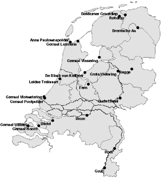
monitored in the water before the pumping station. The locations of the monitoring sites are shown in figure 1. This program monitors the pesticide content in surface water together with ecotoxicological measurements in the same water samples. This makes it possible to

determine whether these pesticides contribute significantly to the toxicity in a number of Dutch surface waters.

(6)

2. Materials and methods

2.1 Sampling method

Four 20 liter stainless steel drums of surface water were collected from each location for ecotoxicological tests, together with two bottles of 1 liter for chemical analysis. Figure 2 shows these drums above the water from the most polluted location "Gemaal Poelpolder" from an area covered with greenhouses. The pesticide concentrations were measured using either gas chromatography coupled with a mass spectrometer [14] or high-performance liquid chromatography with a mass spectrometer [16]. The 20 liter unfiltered surface water from each drum was shaken with 7.5 ml resin XAD 4 and 7.5 ml resin XAD 8. These resins absorb the hydrophobic organic compounds present in the water together with the hydrophobic organic compounds that could be extracted from the particles present in the surface water. The resin was taken out of the water, dried and extracted with acetone. The acetone with the organic micropollutants was stored at -20 °C before the ecotoxicological tests were

performed. A commercial Spring water (Spa blue) was used as a control water. On the day that the toxicity tests were performed, the acetone concentrates were converted to the water phase using a Kuderna-Danish destillation. The water phase (<0.3 ml) was supplemented with EPA medium until a final volume of 60 ml was reached. This is the 1000 times concentrated surface water. The complete concentration method was described previously in more detail [18]. The extraction efficiency was 50% for a moderately hydrophobic pesticide like metoxurone (log Kow = 1.6) and increased to 70% for more hydrophobic pesticides like diuron, azinphos methyl, linuron and triazophos [18].

2.2 Toxicity tests

The concentrate was used in five different toxicity tests. The Daphnia IQ test [8] involves a 75 minutes incubation with Daphnia magna to take up a fluorescent substrate. The Thamnotox test monitors the survival of the crustacean Thamnocephalus platyurus during 24 hours [11, 19, 20]. The test with the rotifer Brachionus calyciflorus also monitors the survival during 24 hours [15]. The Pulse Amplitude Modulation (PAM) test monitors the fluorescence of the photosystem of the green algae Rhapidocelis subcapitata (previously known as Selenastrum capricornutum) during 4.5 hours [7, 9, 10]. The Microtox test monitors the natural

fluorescence of the bacterium Vibrio fisheri for 15 minutes [2]. The highest concentration was the undiluted 1000 times concentrate. Subsequent dilutions of this concentrate were used for a dose effect curve. The EC50 or LC50 is subsequently expressed as y times concentrate [3]. Alternatively, the results can also expressed as Toxic Factors being the inverse of the concentration factor needed to give 50% inhibition.

TF Daphnia = 1/EC50 factor Daphnia {1}

A Toxic Factor of 0.01 for Daphnia for example indicates that the surface water sample had to be concentrated 100 times to inhibit the fluorescence of 50% of the Daphnia. In fact, the 1000 times concentrate was diluted 10 times to inhibit 50% of the Daphnia. The average toxicity of a surface water sample can be expressed as the Geometrical Average of the Toxic Factors of the five toxicity tests (GATF):

GATF = 10^ ((log TF Algea + log TF Microtox + log TF Daphnia + log TF Thamnotox + log TF Rotox)/5) {2}

(7)

The average (µ) and the standard deviation (σ) of a number of logarithmically transformed TF values form the basis of a Species Sensitivity Distribution (SSD). These distributions can be described by the cumulative normal distribution F(x):

(

)

2 2 2 ₂ 2 1 ) ( σ µ πσ − − • =

∫

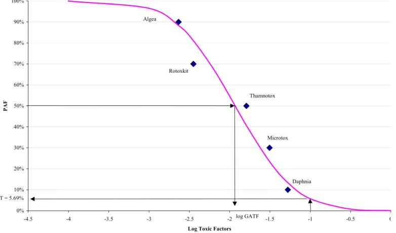
∞ − x e x F x {3} Figure 3 shows, as an example, the log TF values from sample 45. The five toxicity tests are listed in increasing order of toxicity at 90%, 70%, 50%, 30% and 10% to spread the data evenly along the Y axis. The corresponding distribution curve (Potentially Affected Fraction) PAF= 100% - %F(x) shown in figure 3, is derived from the Toxic Factors of these five tests. If another test would be performed with the water from this sampling location, figure 3 indicates that the chance that the EC50 would be more than 1 toxic unit (log TF =0) would be <0.1 %. For the purpose of environmental protection, the chance that the No Observed Effect Concentration (NOEC) exceeds 1 toxic unit is more interesting. It is found that on average for many substances NOEC = EC50/10 [3]. Therefore this chance is found at log TF = -1. This chance is called the pT value (potential Toxicity) [5] and is 5.69 % for sample 45. This indicates a chance of approximately 5.69 % that the NOEC of a species is exceeded in the surface water from sample 45. In the next paragraph, this measured average toxicity GATF, and the measured potential Toxicity pT, will be compared with the average toxicity calculated from the concentrations of the pesticides present in these surface water samples.

2.3 The prediction of toxic effects based on pesticide

concentrations

The correlation between the amount of pesticides and toxic effects in surface waters can be obscured by the presence of other toxicants that are not measured, but do exhibit toxic effects. Therefore, the occurrence of toxicity in the absence of pesticides can hardly be a surprise. However, when pesticides are measured, one should expect toxic effects when the pesticides can be recovered by the XAD method. This is probably the case for pesticides with log Kow> 1.6 which are recovered for more than 50% [18]. For less hydrophobic pesticides the recovery is probably less than 50%. The prediction of the toxicity of a long list of pesticides present in µg/l concentrations is not straightforward because each pesticide exhibits a specific toxicity for a specific test organism. The EC50 values of the pesticides for different aquatic species were obtained by a literature search on various databases. Since 922 EC50 values are used for the different pesticides, the references for each specific EC50 value will be omitted.

2.3.1 Calculation of Toxic Units

The Toxic Unit approach makes it possible to compare the toxicity of different compounds. The ratio between the measured concentration and the EC50 of a specific toxicant for a test species is a dimensionless ratio expressed as Toxic Units [1]. The total toxicity of complex mixtures for a single test species can often be predicted using the rule of concentration addition [21].

TTU = ∑ Cn/EC50n {4}

TTU = Total Toxic Units

Cn= concentration of compound number n

(8)

When for example, the total toxicity of a complex mixture of chemicals adds up to 1 TTU for a single test species it is assumed that 50% of the individuals of the test species is affected. When the toxicity for a whole community of test species has to be evaluated a slightly

different approach is needed. Instead of taking the EC50 of a single species, it is better to take the geometrical average of the EC50 values of a number of species. The geometrical average is favored above the normal average of the EC50 values because the logarithmically

transformed EC50 values of different species are distributed symmetrically in species sensitivity distributions [13]. The geometrical average EC50 gives a reasonable

approximation of the modal EC50 value and is therefore a good representation of the toxicity of a given compound on a number of species. When for example, the total toxicity of a complex mixture of chemicals adds up to 1 TTU for a community of species it is assumed that 50% of the test species are affected for more than 50% of the individuals from each species.

2.3.2 Calculation of the Potentially Affected Fraction

When the toxicity of compounds with different toxic modes of action are calculated, the rule of response addition can be used [21]. The remainder of this paragraph describes this

procedure in short since it was explained in much more detail recently [21]. The toxicity of compounds with a similar mode of action is added up according to equation [4]. This yields the TTU for herbicides, fungicides and insecticides. These three different TTU values are subsequently filled in equation [3] with x = log TTU and an average of µ = -1 [21]. An average µ = -1 instead of µ = 0 is used to convert EC50 values in NOEC values since on average log (NOEC/EC50) = -1 [5]. The standard deviation σ is equal to the average standard deviation of the logarithmically transformed TU values of either the herbicides, fungicides or insecticides [21]. The outcome of equation [3] is called Potentially Affected Fraction

(PAF)and can be interpreted as the chance that a species is affected. When for example, the total toxicity of a complex mixture of chemicals adds up to 0.1 TTU for a community of species it is assumed that 50% of the test species are affected above their NOEC level. The combined effects of herbicides, fungicides and insecticides are calculated using: PAF =1 - (1 - PAF herbicides)*(1 - PAF fungicides)*(1 - PAF insecticides)

(9)

3. Results

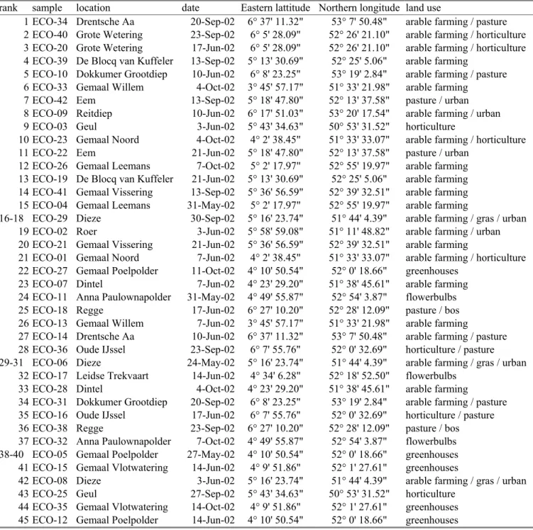
Table 1 shows the sampling locations in different waterways in the Netherlands. The samples in table 1 are ranked in order of increasing average calculated toxicity of pesticides. The method of ranking will be explained in the next paragraphs. Table 1 shows that the waterways near greenhouses rank among the more toxic ones since they have a higher rank number. It also shows that the sampling date is very important since samples from the same location do not rank together. The ECO numbers refer to specific freshwater samples taken at a specific time. From each of the ECO samples ECO-05, ECO-06 and ECO-29 three different

concentrates were made and used for toxicity tests. The chemical analyses were just

performed once for each ECO-sample. Therefore sample rank number 16, 17 and 18 have the same chemical analysis. The same holds true for sample rank number 29, 30, 31 and also for 38, 39 and 40.

3.1 Pesticide analysis of surface water

One of the main disadvantages of ecotoxicological risk assessment based on chemical analysis is the requirement of prior knowledge about the specific chemicals that might contribute to the risk. A decision has to be made which chemicals will be measured. In the case of pesticides in surface waters this decision is difficult because about 900 different pesticides are allowed on the market in Europe

(http://europa.eu.int/comm/food/plant/protection/evaluation/). A selection of pesticides based on the Dutch pesticide use in 1998, emission to surface water and toxicity for aquatic

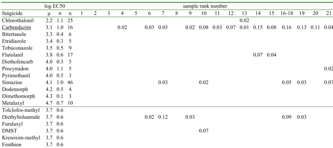
organisms [6] was made. This yielded a list of 120 pesticides from which a further selection of 53 pesticides was made based on high usage and toxicity. Non-hydrophobic pesticides, like for example fentin-acetate and maneb, were omitted because these would not concentrate on the XAD resin used for the toxicity experiments. This selection of pesticides is very different from a selection made in 2003 [4] because the usage patterns of pesticides changes from year-to-year. Table 2 shows the pesticide concentration of the selected 53 pesticides (expressed in µg/liter) together with the Species Sensitivity Distribution formed by the log EC50 values (expressed in µg/liter). For practical reasons, the table is separated in a part for fungicides, herbicides and insecticides, each for the less toxic samples (1 -21) and the more toxic samples. The blank pesticide concentrations are below the detection limit that ranged from 0.01 through 0.05 µg/liter. The sample rank numbers refer to table 1. Samples from the same location show very different pesticide concentrations at different months. For example, the Dieze was sampled three times; sample 16-18 refers to ECO-29 from September , sample 29-31 refers to ECO-06 from May and sample 42 refers to ECO-08 from June. Table 2 shows that the latter sample contains the highest amounts of pesticides and is very different from the samples from September or May. The importance of the sampling date was expected since pesticides can be removed from the water phase by dilution, sorption, biodegradation and other processes.

3.1.1 The problem of the detection limits

Table 2 shows that most measurements were below the detection limit (these are indicated as blank cells). In theory, it is possible that the concentrations below the detection limits can also add up to a considerable contribution to the toxicity. We used a concentration of 50% of the detection limit as a worst-case estimate of the contribution of these low concentrations to the total toxicity expressed as Total Toxic Units. The worst-case occurs for Terbutryne since this herbicide has the lowest EC50 of 10 0.9 =8 µg/liter with a detection limit of 0.01 µg/liter. Half of this amounts to 0.005/8= 0.06% TU which is relatively low compared to the TTU of each

(10)

sample. The contribution of 50 % of the detection limit to the TTU of the other pesticides is one or two orders of magnitude lower since the EC50 of these pesticides is much higher. This shows that the detection limit has little influence on the TTU. For the PAF however, there is some influence of the detection limit. For the PAF calculations we replaced the concentrations below the detection limit for 50 % of the detection limit in order to avoid zero values which gives problems with a logarithmic transformation. This replacement has a strong influence on the low PAF values because the minimal PAF value of 5% is determined by this choice. If we would replace the concentrations below the detection limit for 0.001% of the detection limit the PAF values of 5% would drop to 0%.

3.1.2 The problem of the missing EC50 values

The log EC50 values for a number of species for a specific pesticide form a Species

Sensitivity Distribution with an average µ and a standard deviation σ. In table 2a and 2b, the rows from chlorothalonil through metalaxyl show the fungicides in increasing order of toxicity. These fungicides have a geometrical average EC50 of 103.74 mg/liter. The average log EC50 =3.74 and the standard deviation was 0.6. This average log EC50 is assigned to the remaining fungicides (tolclofos-methyl through fenthion) because we did not have sufficient toxicity data. In table 2c and 2d, the rows from terbutryne through bentazone show the herbicides in increasing order of toxicity. These herbicides have a geometrical average EC50 of 103.69 mg/liter, which is assigned to the remaining herbicides (MCPP through triadimenol). In table 2e and 2f, the rows from parathion through metamitron show the insecticides in increasing order of toxicity. These insecticides have a geometrical average EC50 of 103 mg/liter, which is assigned to the remaining insecticides THPI and tetradifon. This assigning of a geometrical average EC50 introduces a large uncertainty in the contribution of these pesticides to the total toxicity. Fortunately, the concentrations of these pesticides, without a known EC50, were generally very low. It will be shown in the next paragraphs that these pesticides did not contribute much to the total toxicity.

3.1.3 The calculation of the expected toxicity TTU

The ratio between the concentration and the EC50 is a measure of toxicity (see equation 4). This ratio is shown in table 3 and is expressed in ‰ Toxic Units. The Total Toxic Units are the sum of the values in each column. The most toxic sample (number 45 from Gemaal Poelpolder) showed 5.2‰ TTU fungicides , 0.1‰ TTU herbicides and 73.1‰ TTU insecticides giving 78.4‰ TTU. This indicates that the sample must be concentrated 1/0.0784 = 13 times to inhibit the "geometrical average" species for 50%. The less toxic sample number 10 showed 0.1 ‰TTU and must therefore be concentrated 10,000 times to inhibit the "geometrical average" species for 50%. This indicates that the toxicity of pesticides in the samples can be expected to be relatively low even in the 1000 times concentrated samples. Only for samples 27 through 45 might it be possible to measure toxic effects of pesticides after a concentration step of 1000 times.

3.1.4 The influence of the assigned EC50 values

Table 3 shows that the pesticides with an unknown EC50 value did not contribute largely to the total toxicity. Generally, their estimated contribution to toxicity is lower than 0.1 ‰ Toxic Units. Only THPI showed a significant contribution of 0.4 ‰, 0.7 ‰ and 2‰ TU to samples 32, 38 and 37, respectively.

(11)

3.2 Comparison between measured and calculated toxicity

At this stage the TTU herbicides, TTU fungicides and the TTU insecticides can either be added up to a total TTU or they can be combined using the response addition according to equation 5. This combination yields the PAF that can be interpreted as the chance that a species is affected at the measured pesticide concentrations in a surface water sample. This PAF can be compared with the pT value that can be interpreted as the chance that a species is affected in a not concentrated surface water sample. In a previous report the pT of a defined mixture of pesticides or surfactants correlated well with the calculated PAF based on the concentrations of either pesticides or surfactants [17]. In this report however, undefined surface water samples were used which might also contain other toxic compounds (including not measured pesticides) apart from the list of measured pesticides.

The comparison between the pT and the PAF is hampered by a relatively large uncertainty since both are dependent on the average and the standard deviation of the measurements. In contrast, the comparison between the GATF and the TTU is dependent on the average of the measurements. The GATF is calculated from the geometric average of the toxicity factors and the TTU is calculated from the measured pesticide concentrations divided by the geometric average of the EC50 values for each pesticide.

Figure 4a shows the TF of each of the five tests and figure 4b compares the calculated PAF and TTU with the measured toxicity pT and GATF. For the first 44 samples, TTU is much larger than GATF. This shows that most of the toxicity in these samples is not caused by the measured pesticides. The first 13 samples, which have the lowest calculated toxicity GATF and therefore the lowest concentrations of pesticides, do not show high TF values (> 2%) for any test. This is remarkable because high TF values are quite common in the latter samples. This indicates that there might be a correlation between pesticide use and surface water toxicity. Since the above calculation showed no direct relation, it might be possible that there is an indirect correlation. Low concentrations of the selected list of pesticides might be correlated with less intensive agriculture which might in its turn be correlated with less surface water pollution.

Table 4 is a tabulated form of figure 4. It is however not sorted using TTU but sorted using the sampling locations from North two South. This facilitates a comparison between different samples from the same location. Sample number 16, 17 and 18 are identical samples and therefore show very similar TF, GATF and pT values. The TTU values of 17 and 18 were not measured but it can be assumed that a repetitive chemical analysis of the same sample is very reproducible. The same similarities are shown in sample number 29, 30 and 31 and are also shown in 38, 39 and 40. For comparison purposes, GATF is a more reproducible measure of toxicity compared to pT. For example, the pT value of sample 16 is six times higher than the pT value of sample 18 while both are taken from the same water sample. The GATF value is much less variable than the pT value. The Rotox and Thamnotox tests are generally less sensitive than the other toxicity tests. This was also observed when the concentrates from Dutch rivers were used [5]. The maximal TF of the Rotox test is 0.85% whereas it is close to 5% for the other tests (see table 4). The sampling time is very important and therefore it is very difficult to compare different locations when only a few time points are sampled. For example, Gemaal Poelpolder gave the most polluted sample number 45 but it also gave sample number 22 which is less polluted than sample 27 from the Drentsche Aa. The cleanest sample no. 1 was also taken from the Drentsche Aa. This indicates that it is difficult to

distinguish even the most polluted site from the least polluted site when only two sampling moments are used.

(12)

3.2.1 Sample number 45

In sample number 45 from Gemaal Poelpolder the calculated GATF is higher than the measured TTU. That is the reason why the sample is treated here in more detail. The TF for Daphnia and Microtox of sample 45 is quite similar to the corresponding TF values of sample 18 from the same location measured 18 days earlier, while the pesticide concentrations in sample 45 are more than tenfold higher. The major toxicants in sample 45 are 3.1 µg/l parathion 5.2 µg/l diethofencarb and 6.2 µg/l carbendazim (see table 2). The high amount of parathion poses a problem since we did expect a higher toxicity than the observed toxicity in the sample. The EC50 of parathion for Daphnia magna ranges from 2 to 7 µg/liter (EPA toxicity database). This would yield a TU ranging from 155% to 44% for Daphnia which is much higher than the observed 5.7% shown in figure 1. Theoretically this difference might be attributed to either a bad extraction procedure or a relatively insensitive toxicity test. The extraction procedure performed before the toxicity tests can theoretically remove toxic

compounds that are not hydrophobic. The log Kow of parathion however, ranges from 2.15 to 3.93 which indicates that the extraction efficiency for parathion is expected to be in the range of 70% [18]. Therefore, a low extraction efficiency is not likely to explain the relatively low observed toxicity for Daphnia.

The difference between the traditional Daphnia tests and the rapid Daphnia test performed here is less than a factor three for most compounds [12]. Therefore, the difference between the observed 5.7% and the calculated 44% would be significant foremost compounds. There is however a possibility that the difference between the traditional and the rapid test is higher for parathion. This remains to be tested.

(13)

4. Conclusions

Our results show that the selected pesticides did not make a large contribution to the toxicity of the regional surface water samples. However, occasional peak concentrations of pesticides might exhibit a major contribution to the toxicity at certain locations. The high parathion concentration of 3.1 µg/liter in a sample from Gemaal Poelpolder might be able to cause serious ecological consequences because it is close to the EC50 of Daphnia magna.

However, the measured toxic effects on Daphnia in that sample were significantly lower than the expected toxic effects based on the high parathion concentration. More and more frequent measurements are needed during the summer months in the surface water from Gemaal Poelpolder to confirm these findings. The toxicity and the pesticides concentrations at the studied sites show a large temporal variation. Therefore, frequent measurements at a specific site are needed in order to draw any conclusions about the pollution of the site.

5. Recommendations

Replace one of the negative control samples Spa blue with a positive control containing relatively unpolluted surface water with 5 µg/liter parathion. Use this sample both for chemical and toxicological analysis. Update the list of measured pesticides according to recent usage patterns.

Store the leftover of the concentrates in closed HPLC vessels for future analysis. After some years of sample collection, it might be possible to correlate specific toxic effects with the presence of certain chemicals in the surface water concentrates.

Much more frequent sampling is needed to compare the pesticide pollution and the toxic effects at different sites.

Acknowledgments

The authors thank J. Struijs and T. Breure for valuable comments on a draft version of this report. They also thank A.M.A. van der Linden for help with the selection of pesticides, S. Simpson for correcting the English , and A. Rooseboom-Reimers, A.A.M. Stolker and W. Niesing for pesticide analysis.

(14)

Figure 1 The position of the sampling locations in the Netherlands

(15)

0% 10% 20% 30% 40% 50% 60% 70% 80% 90% 100% -4.5 -4 -3.5 -3 -2.5 -2 -1.5 -1 -0.5 0

Log Toxic Factors

PAF Rotoxkit Algea Thamnotox Microtox Daphnia pT = 5.69% log GATF

Figure 3 An illustration of the calculation of the toxic potency (pT) from the Toxic Factor values of five toxicity tests, in this example for sample 45

(16)

Table 1. The freshwater samples ranked in order of increasing calculated pesticide toxicity (Total Toxic Units)

rank sample location date Eastern lattitude Northern longitude land use

1 ECO-34 Drentsche Aa 20-Sep-02 6° 37' 11.32" 53° 7' 50.48" arable farming / pasture 2 ECO-40 Grote Wetering 23-Sep-02 6° 5' 28.09" 52° 26' 21.10" arable farming / horticulture 3 ECO-20 Grote Wetering 17-Jun-02 6° 5' 28.09" 52° 26' 21.10" arable farming / horticulture 4 ECO-39 De Blocq van Kuffeler 13-Sep-02 5° 13' 30.69" 52° 25' 5.06" arable farming

5 ECO-10 Dokkumer Grootdiep 10-Jun-02 6° 8' 23.25" 53° 19' 2.84" arable farming / pasture 6 ECO-33 Gemaal Willem 4-Oct-02 3° 45' 57.17" 51° 33' 21.98" arable farming

7 ECO-42 Eem 13-Sep-02 5° 18' 47.80" 52° 13' 37.58" pasture / urban 8 ECO-09 Reitdiep 10-Jun-02 6° 17' 51.03" 53° 20' 17.54" arable farming / urban 9 ECO-03 Geul 3-Jun-02 5° 43' 34.63" 50° 53' 31.52" horticulture

10 ECO-23 Gemaal Noord 4-Oct-02 4° 2' 38.45" 51° 33' 33.07" arable farming / horticulture 11 ECO-22 Eem 21-Jun-02 5° 18' 47.80" 52° 13' 37.58" pasture / urban

12 ECO-26 Gemaal Leemans 7-Oct-02 5° 2' 17.97" 52° 55' 19.97" arable farming 13 ECO-19 De Blocq van Kuffeler 21-Jun-02 5° 13' 30.69" 52° 25' 5.06" arable farming 14 ECO-41 Gemaal Vissering 13-Sep-02 5° 36' 56.59" 52° 39' 32.51" arable farming 15 ECO-04 Gemaal Leemans 31-May-02 5° 2' 17.97" 52° 55' 19.97" arable farming

16-18 ECO-29 Dieze 30-Sep-02 5° 16' 23.74" 51° 44' 4.39" arable farming / gras / urban 19 ECO-02 Roer 3-Jun-02 5° 58' 59.08" 51° 11' 48.82" arable farming / urban 20 ECO-21 Gemaal Vissering 21-Jun-02 5° 36' 56.59" 52° 39' 32.51" arable farming

21 ECO-01 Gemaal Noord 7-Jun-02 4° 2' 38.45" 51° 33' 33.07" arable farming / horticulture 22 ECO-27 Gemaal Poelpolder 11-Oct-02 4° 10' 50.54" 52° 0' 18.66" greenhouses

23 ECO-07 Dintel 7-Jun-02 4° 23' 29.20" 51° 38' 45.61" arable farming 24 ECO-11 Anna Paulownapolder 31-May-02 4° 49' 55.87" 52° 54' 3.87" flowerbulbs 25 ECO-18 Regge 17-Jun-02 6° 27' 10.20" 52° 28' 12.09" pasture / bos 26 ECO-13 Gemaal Willem 7-Jun-02 3° 45' 57.17" 51° 33' 21.98" arable farming

27 ECO-14 Drentsche Aa 10-Jun-02 6° 37' 11.32" 53° 7' 50.48" arable farming / pasture 28 ECO-36 Oude IJssel 23-Sep-02 6° 7' 55.76" 52° 0' 32.69" horticulture / pasture 29-31 ECO-06 Dieze 24-May-02 5° 16' 23.74" 51° 44' 4.39" arable farming / gras / urban

32 ECO-17 Leidse Trekvaart 14-Jun-02 4° 34' 6.28" 52° 18' 52.50" flowerbulbs 33 ECO-28 Dintel 4-Oct-02 4° 23' 29.20" 51° 38' 45.61" arable farming

34 ECO-31 Dokkumer Grootdiep 20-Sep-02 6° 8' 23.25" 53° 19' 2.84" arable farming / pasture 35 ECO-16 Oude IJssel 17-Jun-02 6° 7' 55.76" 52° 0' 32.69" horticulture / pasture 36 ECO-38 Regge 23-Sep-02 6° 27' 10.20" 52° 28' 12.09" pasture / bos 37 ECO-32 Anna Paulownapolder 7-Oct-02 4° 49' 55.87" 52° 54' 3.87" flowerbulbs 38-40 ECO-05 Gemaal Poelpolder 27-May-02 4° 10' 50.54" 52° 0' 18.66" greenhouses 41 ECO-15 Gemaal Vlotwatering 14-Jun-02 4° 9' 51.86" 52° 1' 27.61" greenhouses

42 ECO-08 Dieze 3-Jun-02 5° 16' 23.74" 51° 44' 4.39" arable farming / gras / urban 43 ECO-25 Geul 27-Sep-02 5° 43' 34.63" 50° 53' 31.52" horticulture

44 ECO-35 Gemaal Vlotwatering 14-Oct-02 4° 9' 51.86" 52° 1' 27.61" greenhouses 45 ECO-12 Gemaal Poelpolder 14-Jun-02 4° 10' 50.54" 52° 0' 18.66" greenhouses

(17)

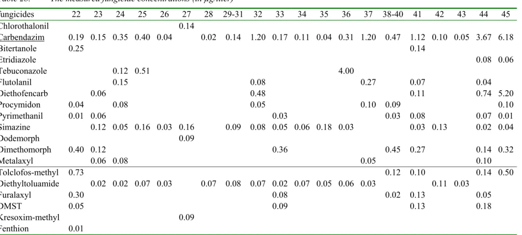
Table 2a. The measured fungicide concentrations and the sensitivity distribution of the log EC50 values (all in µg/liter)

log EC50 sample rank number

fungicide µ σ n 1 2 3 4 5 6 7 8 9 10 11 12 13 14 15 16-18 19 20 21 Chlorothalonil 2.2 1.1 25 0.00 0.00 0.00 0.00 0.00 0.00 0.00 0.00 0.00 0.00 0.00 0.00 0.02 0.00 0.00 0.00 0.00 0.00 0.00 Carbendazim 3.1 1.0 16 0.00 0.00 0.00 0.02 0.00 0.03 0.03 0.00 0.02 0.08 0.03 0.07 0.01 0.15 0.08 0.16 0.13 0.11 0.04 Bitertanole 3.3 0.4 6 0.00 0.00 0.00 0.00 0.00 0.00 0.00 0.00 0.00 0.00 0.00 0.00 0.00 0.00 0.00 0.00 0.00 0.00 0.00 Etridiazole 3.4 0.3 5 0.00 0.00 0.00 0.00 0.00 0.00 0.00 0.00 0.00 0.00 0.00 0.00 0.00 0.00 0.00 0.00 0.00 0.00 0.00 Tebuconazole 3.5 0.5 9 0.00 0.00 0.00 0.00 0.00 0.00 0.00 0.00 0.00 0.00 0.00 0.00 0.00 0.00 0.00 0.00 0.00 0.00 0.00 Flutolanil 3.8 0.6 17 0.00 0.00 0.00 0.00 0.00 0.00 0.00 0.00 0.00 0.00 0.00 0.00 0.00 0.07 0.04 0.00 0.00 0.00 0.00 Diethofencarb 4.0 0.3 5 0.00 0.00 0.00 0.00 0.00 0.00 0.00 0.00 0.00 0.00 0.00 0.00 0.00 0.00 0.00 0.00 0.00 0.00 0.00 Procymidon 4.0 1.1 5 0.00 0.00 0.00 0.00 0.00 0.00 0.00 0.00 0.00 0.00 0.00 0.00 0.00 0.00 0.00 0.00 0.00 0.00 0.02 Pyrimethanil 4.0 0.5 3 0.00 0.00 0.00 0.00 0.00 0.00 0.00 0.00 0.00 0.00 0.00 0.00 0.00 0.00 0.00 0.00 0.00 0.00 0.00 Simazine 4.1 1.0 46 0.00 0.00 0.00 0.00 0.00 0.00 0.03 0.00 0.00 0.02 0.00 0.00 0.00 0.00 0.00 0.05 0.03 0.00 0.07 Dodemorph 4.2 0.5 4 0.00 0.00 0.00 0.00 0.00 0.00 0.00 0.00 0.00 0.00 0.00 0.00 0.00 0.00 0.00 0.00 0.00 0.00 0.00 Dimethomorph 4.3 0.1 3 0.00 0.00 0.00 0.00 0.00 0.00 0.00 0.00 0.00 0.00 0.00 0.00 0.00 0.00 0.00 0.00 0.00 0.00 0.00 Metalaxyl 4.7 0.7 10 0.00 0.00 0.00 0.00 0.00 0.00 0.00 0.00 0.00 0.00 0.00 0.00 0.00 0.00 0.00 0.00 0.00 0.00 0.00 Tolclofos-methyl 3.7 0.6 0.00 0.00 0.00 0.00 0.00 0.00 0.00 0.00 0.00 0.00 0.00 0.00 0.00 0.00 0.00 0.00 0.00 0.00 0.00 Diethyltoluamide 3.7 0.6 0.00 0.00 0.00 0.00 0.00 0.02 0.12 0.00 0.03 0.00 0.00 0.00 0.00 0.00 0.00 0.09 0.03 0.00 0.00 Furalaxyl 3.7 0.6 0.00 0.00 0.00 0.00 0.00 0.00 0.00 0.00 0.00 0.00 0.00 0.00 0.00 0.00 0.00 0.00 0.00 0.00 0.00 DMST 3.7 0.6 0.00 0.00 0.00 0.00 0.00 0.00 0.00 0.00 0.00 0.07 0.00 0.00 0.00 0.00 0.00 0.00 0.00 0.00 0.00 Kresoxim-methyl 3.7 0.6 0.00 0.00 0.00 0.00 0.00 0.00 0.00 0.00 0.00 0.00 0.00 0.00 0.00 0.00 0.00 0.00 0.00 0.00 0.00 Fenthion 3.7 0.6 0.00 0.00 0.00 0.00 0.00 0.00 0.00 0.00 0.00 0.00 0.00 0.00 0.00 0.00 0.00 0.00 0.00 0.00 0.00

*_{The rows are sorted with increasing EC50 values except for the last six rows which have an estimated EC50 value. Average µ, standard}

deviation σ, number n of log EC50 values. The underlined pesticides are measured using LC MS [16], while the others are measured using GC MS [14]

(18)

Table 2b. The measured fungicide concentrations (in µg/liter) fungicides 22 23 24 25 26 27 28 29-31 32 33 34 35 36 37 38-40 41 42 43 44 45 Chlorothalonil 0.00 0.00 0.00 0.00 0.00 0.14 0.00 0.00 0.00 0.00 0.00 0.00 0.00 0.00 0.00 0.00 0.00 0.00 0.00 0.00 Carbendazim 0.19 0.15 0.35 0.40 0.04 0.00 0.02 0.14 1.20 0.17 0.11 0.04 0.31 1.20 0.47 1.12 0.10 0.05 3.67 6.18 Bitertanole 0.25 0.00 0.00 0.00 0.00 0.00 0.00 0.00 0.00 0.00 0.00 0.00 0.00 0.00 0.00 0.14 0.00 0.00 0.00 0.00 Etridiazole 0.00 0.00 0.00 0.00 0.00 0.00 0.00 0.00 0.00 0.00 0.00 0.00 0.00 0.00 0.00 0.00 0.00 0.00 0.08 0.06 Tebuconazole 0.00 0.00 0.12 0.51 0.00 0.00 0.00 0.00 0.00 0.00 0.00 0.00 4.00 0.00 0.00 0.00 0.00 0.00 0.00 0.00 Flutolanil 0.00 0.00 0.15 0.00 0.00 0.00 0.00 0.00 0.08 0.00 0.00 0.00 0.00 0.27 0.00 0.07 0.00 0.00 0.04 0.00 Diethofencarb 0.00 0.06 0.00 0.00 0.00 0.00 0.00 0.00 0.48 0.00 0.00 0.00 0.00 0.00 0.00 0.11 0.00 0.00 0.74 5.20 Procymidon 0.04 0.00 0.08 0.00 0.00 0.00 0.00 0.00 0.05 0.00 0.00 0.00 0.00 0.10 0.09 0.00 0.00 0.00 0.00 0.10 Pyrimethanil 0.01 0.06 0.00 0.00 0.00 0.00 0.00 0.00 0.00 0.03 0.00 0.00 0.00 0.00 0.03 0.08 0.00 0.00 0.07 0.01 Simazine 0.00 0.12 0.05 0.16 0.03 0.16 0.00 0.09 0.08 0.05 0.06 0.18 0.03 0.00 0.00 0.03 0.13 0.00 0.02 0.04 Dodemorph 0.00 0.00 0.00 0.00 0.00 0.09 0.00 0.00 0.00 0.00 0.00 0.00 0.00 0.00 0.00 0.00 0.00 0.00 0.00 0.00 Dimethomorph 0.40 0.12 0.00 0.00 0.00 0.00 0.00 0.00 0.00 0.36 0.00 0.00 0.00 0.00 0.45 0.27 0.00 0.00 0.14 0.32 Metalaxyl 0.00 0.06 0.08 0.00 0.00 0.00 0.00 0.00 0.00 0.00 0.00 0.00 0.00 0.05 0.00 0.00 0.00 0.00 0.10 0.00 Tolclofos-methyl 0.73 0.00 0.00 0.00 0.00 0.00 0.00 0.00 0.00 0.00 0.00 0.00 0.00 0.00 0.12 0.10 0.00 0.00 0.14 0.50 Diethyltoluamide 0.00 0.02 0.02 0.07 0.03 0.00 0.07 0.08 0.07 0.02 0.07 0.05 0.06 0.03 0.00 0.00 0.11 0.03 0.00 0.00 Furalaxyl 0.30 0.00 0.00 0.00 0.00 0.00 0.00 0.00 0.00 0.08 0.00 0.00 0.00 0.00 0.02 0.13 0.00 0.00 0.05 0.00 DMST 0.05 0.00 0.00 0.00 0.00 0.00 0.00 0.00 0.00 0.09 0.00 0.00 0.00 0.00 0.00 0.13 0.00 0.00 0.18 0.00 Kresoxim-methyl 0.00 0.00 0.00 0.00 0.00 0.09 0.00 0.00 0.00 0.00 0.00 0.00 0.00 0.00 0.00 0.00 0.00 0.00 0.00 0.00 Fenthion 0.01 0.00 0.00 0.00 0.00 0.00 0.00 0.00 0.00 0.00 0.00 0.00 0.00 0.00 0.00 0.00 0.00 0.00 0.00 0.00

(19)

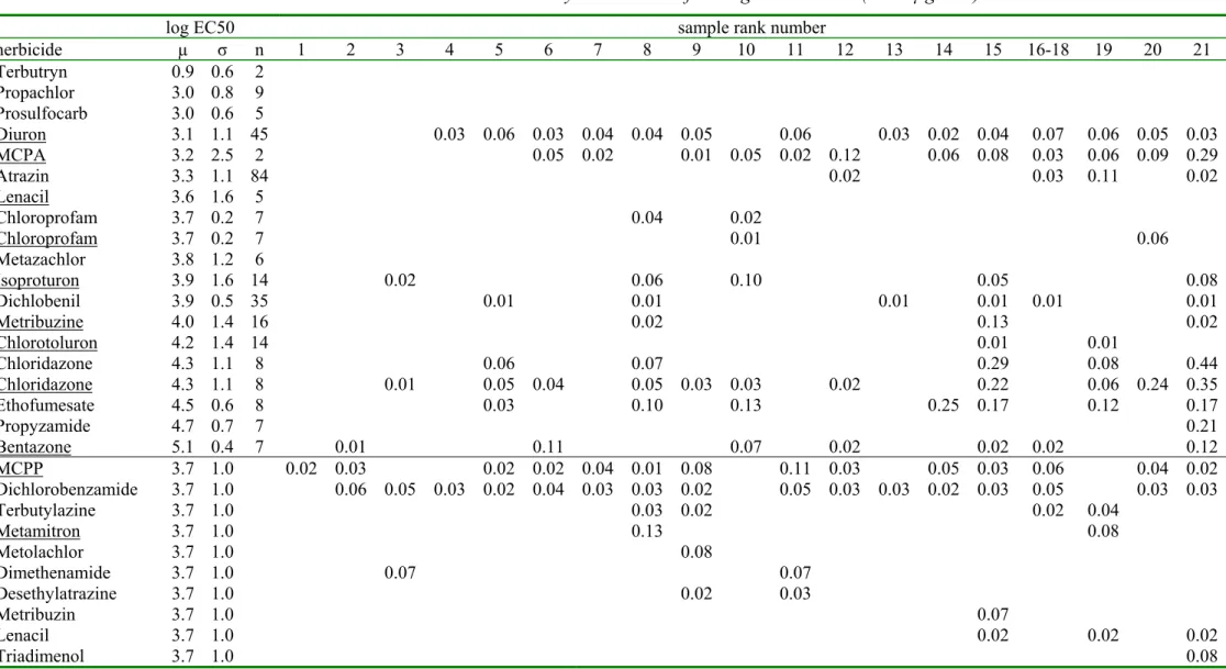
Table 2c. The measured herbicide concentrations and the sensitivity distribution of the log EC50 values (all in µg/liter)

herbicide µ σ n 1 2 3 4 5 6 7 8 9 10 11 12 13 14 15 16-18 19 20 21 Terbutryn 0.9 0.6 2 0.00 0.00 0.00 0.00 0.00 0.00 0.00 0.00 0.00 0.00 0.00 0.00 0.00 0.00 0.00 0.00 0.00 0.00 0.00 Propachlor 3.0 0.8 9 0.00 0.00 0.00 0.00 0.00 0.00 0.00 0.00 0.00 0.00 0.00 0.00 0.00 0.00 0.00 0.00 0.00 0.00 0.00 Prosulfocarb 3.0 0.6 5 0.00 0.00 0.00 0.00 0.00 0.00 0.00 0.00 0.00 0.00 0.00 0.00 0.00 0.00 0.00 0.00 0.00 0.00 0.00 Diuron 3.1 1.1 45 0.00 0.00 0.00 0.03 0.06 0.03 0.04 0.04 0.05 0.00 0.06 0.00 0.03 0.02 0.04 0.07 0.06 0.05 0.03 MCPA 3.2 2.5 2 0.00 0.00 0.00 0.00 0.00 0.05 0.02 0.00 0.01 0.05 0.02 0.12 0.00 0.06 0.08 0.03 0.06 0.09 0.29 Atrazin 3.3 1.1 84 0.00 0.00 0.00 0.00 0.00 0.00 0.00 0.00 0.00 0.00 0.00 0.02 0.00 0.00 0.00 0.03 0.11 0.00 0.02 Lenacil 3.6 1.6 5 0.00 0.00 0.00 0.00 0.00 0.00 0.00 0.00 0.00 0.00 0.00 0.00 0.00 0.00 0.00 0.00 0.00 0.00 0.00 Chloroprofam 3.7 0.2 7 0.00 0.00 0.00 0.00 0.00 0.00 0.00 0.04 0.00 0.02 0.00 0.00 0.00 0.00 0.00 0.00 0.00 0.00 0.00 Chloroprofam 3.7 0.2 7 0.00 0.00 0.00 0.00 0.00 0.00 0.00 0.00 0.00 0.01 0.00 0.00 0.00 0.00 0.00 0.00 0.00 0.06 0.00 Metazachlor 3.8 1.2 6 0.00 0.00 0.00 0.00 0.00 0.00 0.00 0.00 0.00 0.00 0.00 0.00 0.00 0.00 0.00 0.00 0.00 0.00 0.00 Isoproturon 3.9 1.6 14 0.00 0.00 0.02 0.00 0.00 0.00 0.00 0.06 0.00 0.10 0.00 0.00 0.00 0.00 0.05 0.00 0.00 0.00 0.08 Dichlobenil 3.9 0.5 35 0.00 0.00 0.00 0.00 0.01 0.00 0.00 0.01 0.00 0.00 0.00 0.00 0.01 0.00 0.01 0.01 0.00 0.00 0.01 Metribuzine 4.0 1.4 16 0.00 0.00 0.00 0.00 0.00 0.00 0.00 0.02 0.00 0.00 0.00 0.00 0.00 0.00 0.13 0.00 0.00 0.00 0.02 Chlorotoluron 4.2 1.4 14 0.00 0.00 0.00 0.00 0.00 0.00 0.00 0.00 0.00 0.00 0.00 0.00 0.00 0.00 0.01 0.00 0.01 0.00 0.00 Chloridazone 4.3 1.1 8 0.00 0.00 0.00 0.00 0.06 0.00 0.00 0.07 0.00 0.00 0.00 0.00 0.00 0.00 0.29 0.00 0.08 0.00 0.44 Chloridazone 4.3 1.1 8 0.00 0.00 0.01 0.00 0.05 0.04 0.00 0.05 0.03 0.03 0.00 0.02 0.00 0.00 0.22 0.00 0.06 0.24 0.35 Ethofumesate 4.5 0.6 8 0.00 0.00 0.00 0.00 0.03 0.00 0.00 0.10 0.00 0.13 0.00 0.00 0.00 0.25 0.17 0.00 0.12 0.00 0.17 Propyzamide 4.7 0.7 7 0.00 0.00 0.00 0.00 0.00 0.00 0.00 0.00 0.00 0.00 0.00 0.00 0.00 0.00 0.00 0.00 0.00 0.00 0.21 Bentazone 5.1 0.4 7 0.00 0.01 0.00 0.00 0.00 0.11 0.00 0.00 0.00 0.07 0.00 0.02 0.00 0.00 0.02 0.02 0.00 0.00 0.12 MCPP 3.7 1.0 0.02 0.03 0.00 0.00 0.02 0.02 0.04 0.01 0.08 0.00 0.11 0.03 0.00 0.05 0.03 0.06 0.00 0.04 0.02 Dichlorobenzamide 3.7 1.0 0.00 0.06 0.05 0.03 0.02 0.04 0.03 0.03 0.02 0.00 0.05 0.03 0.03 0.02 0.03 0.05 0.00 0.03 0.03 Terbutylazine 3.7 1.0 0.00 0.00 0.00 0.00 0.00 0.00 0.00 0.03 0.02 0.00 0.00 0.00 0.00 0.00 0.00 0.02 0.04 0.00 0.00 Metamitron 3.7 1.0 0.00 0.00 0.00 0.00 0.00 0.00 0.00 0.13 0.00 0.00 0.00 0.00 0.00 0.00 0.00 0.00 0.08 0.00 0.00 Metolachlor 3.7 1.0 0.00 0.00 0.00 0.00 0.00 0.00 0.00 0.00 0.08 0.00 0.00 0.00 0.00 0.00 0.00 0.00 0.00 0.00 0.00 Dimethenamide 3.7 1.0 0.00 0.00 0.07 0.00 0.00 0.00 0.00 0.00 0.00 0.00 0.07 0.00 0.00 0.00 0.00 0.00 0.00 0.00 0.00 Desethylatrazine 3.7 1.0 0.00 0.00 0.00 0.00 0.00 0.00 0.00 0.00 0.02 0.00 0.03 0.00 0.00 0.00 0.00 0.00 0.00 0.00 0.00 Metribuzin 3.7 1.0 0.00 0.00 0.00 0.00 0.00 0.00 0.00 0.00 0.00 0.00 0.00 0.00 0.00 0.00 0.07 0.00 0.00 0.00 0.00 Lenacil 3.7 1.0 0.00 0.00 0.00 0.00 0.00 0.00 0.00 0.00 0.00 0.00 0.00 0.00 0.00 0.00 0.02 0.00 0.02 0.00 0.02 Triadimenol 3.7 1.0 0.00 0.00 0.00 0.00 0.00 0.00 0.00 0.00 0.00 0.00 0.00 0.00 0.00 0.00 0.00 0.00 0.00 0.00 0.08

deviation σ , number n of log EC50 values. The underlined pesticides are measured using LC MS [16], while the others are measured using

(20)

Table 2d. The measured herbicide concentrations (in µg/liter) herbicide 22 23 24 25 26 27 28 29-31 32 33 34 35 36 37 38-40 41 42 43 44 45 Terbutryn 0.00 0.00 0.00 0.00 0.00 0.00 0.01 0.01 0.00 0.01 0.01 0.02 0.01 0.00 0.00 0.00 0.03 0.04 0.00 0.00 Propachlor 0.00 0.01 0.00 0.00 0.00 0.00 0.00 0.00 0.02 0.00 0.00 0.00 0.00 0.00 0.07 0.00 0.00 0.00 0.00 0.02 Prosulfocarb 0.00 0.04 0.00 0.00 0.00 0.00 0.00 0.05 0.00 0.00 0.00 0.00 0.00 0.00 0.34 0.00 0.04 0.00 0.00 0.03 Diuron 0.00 0.21 0.03 0.09 0.23 0.00 0.02 0.07 0.04 0.10 0.08 0.07 0.02 0.00 0.00 0.04 0.15 0.12 0.00 0.00 MCPA 0.00 0.00 0.03 0.04 0.00 0.04 0.01 0.03 0.09 0.06 0.05 0.02 0.02 0.04 0.03 0.01 0.04 0.06 0.01 0.02 Atrazin 0.00 0.04 0.01 0.06 1.00 0.00 0.00 0.04 0.01 0.04 0.00 0.02 0.00 0.00 0.06 0.03 0.07 0.08 0.00 0.05 Lenacil 0.00 0.00 0.05 0.00 0.00 0.00 0.00 0.00 0.00 0.00 0.00 0.00 0.00 0.00 0.00 0.00 0.00 0.00 0.00 0.00 Chloroprofam 0.00 0.04 0.10 0.00 0.00 0.00 0.00 0.05 0.05 0.00 0.00 0.00 0.00 0.00 0.09 0.00 0.06 0.00 0.08 0.02 Chloroprofam 0.00 0.00 0.01 0.00 0.00 0.00 0.00 0.01 0.02 0.00 0.00 0.00 0.00 0.00 0.00 0.00 0.02 0.00 0.03 0.00 Metazachlor 0.00 0.03 0.00 0.00 0.00 0.00 0.00 0.00 0.00 0.03 0.00 0.00 0.00 0.00 0.00 0.05 0.00 0.00 0.00 0.00 Isoproturon 0.00 0.00 0.00 0.00 0.00 0.00 0.00 0.00 0.00 0.00 0.00 0.00 0.00 0.00 0.00 0.00 0.00 0.01 0.00 0.00 Dichlobenil 0.00 0.02 0.02 0.02 0.02 0.00 0.01 0.02 0.02 0.00 0.01 0.02 0.00 0.00 0.06 0.03 0.03 0.05 0.02 0.02 Metribuzine 0.00 0.04 0.00 0.00 0.00 0.00 0.00 0.00 0.00 0.00 0.00 0.00 0.00 0.00 0.00 0.00 0.09 0.00 0.00 0.00 Chlorotoluron 0.00 0.00 0.00 0.00 0.00 0.00 0.00 0.00 0.00 0.00 0.00 0.00 0.00 0.00 0.00 0.00 0.00 0.00 0.00 0.00 Chloridazone 0.00 0.70 0.92 0.00 0.15 0.00 0.00 0.00 0.05 0.00 0.00 0.00 0.00 0.14 0.00 0.00 0.09 0.00 0.00 0.00 Chloridazone 0.00 0.54 0.67 0.00 0.11 0.00 0.00 0.04 0.06 0.02 0.00 0.01 0.00 0.11 0.02 0.00 0.06 0.00 0.00 0.00 Ethofumesate 0.00 0.42 0.00 0.00 0.04 0.00 0.00 0.20 0.00 0.00 0.00 0.13 0.00 0.00 0.12 0.00 0.26 0.00 0.00 0.00 Propyzamide 0.00 0.04 0.00 0.00 0.04 0.00 0.00 0.00 0.00 0.00 0.00 0.00 0.00 0.00 0.04 0.00 0.00 0.00 0.00 0.00 Bentazone 0.00 0.03 0.00 0.01 0.08 0.00 0.02 0.03 0.08 0.03 0.00 0.00 0.01 0.13 0.00 0.00 0.05 0.00 0.00 0.00 MCPP 0.01 0.03 0.03 0.10 0.03 0.04 0.01 0.06 0.05 0.04 0.04 0.02 0.04 0.06 0.05 0.03 0.08 0.09 0.03 0.00 Dichlorobenzamide 0.04 0.04 0.06 0.04 0.06 0.00 0.00 0.05 0.10 0.04 0.04 0.03 0.04 0.04 0.04 0.07 0.05 0.03 0.08 0.04 Terbutylazine 0.00 0.02 0.00 0.16 0.16 0.02 0.00 0.02 0.00 0.05 0.00 0.12 0.02 0.00 0.00 0.01 0.10 0.00 0.00 0.01 Metamitron 0.00 0.00 0.15 0.00 0.00 0.00 0.00 0.06 0.00 0.00 0.00 0.07 0.00 0.00 0.00 0.00 0.00 0.00 0.12 0.00 Metolachlor 0.00 0.06 0.00 0.06 0.00 0.00 0.00 0.03 0.00 0.07 0.00 0.11 0.00 0.00 0.03 0.00 0.05 0.00 0.00 0.01 Dimethenamide 0.00 0.00 0.00 0.00 0.00 0.00 0.00 0.00 0.00 0.00 0.00 0.10 0.00 0.00 0.00 0.00 0.06 0.00 0.00 0.00 Desethylatrazine 0.00 0.02 0.00 0.01 0.01 0.00 0.00 0.00 0.00 0.02 0.00 0.00 0.00 0.00 0.04 0.03 0.03 0.01 0.00 0.04 Metribuzin 0.00 0.02 0.00 0.00 0.00 0.00 0.00 0.02 0.00 0.00 0.00 0.00 0.00 0.00 0.00 0.00 0.03 0.00 0.00 0.00 Lenacil 0.00 0.00 0.02 0.00 0.00 0.00 0.00 0.00 0.00 0.00 0.00 0.00 0.00 0.00 0.02 0.00 0.00 0.00 0.00 0.00 Triadimenol 0.00 0.00 0.00 0.00 0.00 0.00 0.00 0.00 0.00 0.00 0.00 0.00 0.00 0.00 0.00 0.00 0.00 0.00 0.00 0.00

(21)

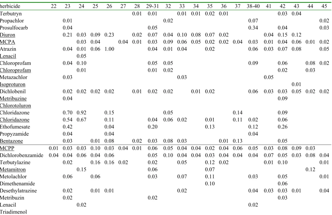
Table 2e. The measured insecticide concentrations and the sensitivity distribution of the log EC50 values (all in µg/liter)

insecticide µ σ n 1 2 3 4 5 6 7 8 9 10 11 12 13 14 15 16-18 19 20 21 Parathion 1.6 1.4 114 0.00 0.00 0.00 0.00 0.00 0.00 0.00 0.00 0.00 0.00 0.00 0.00 0.00 0.00 0.00 0.00 0.00 0.00 0.00 Diazinon 2.2 1.4 81 0.00 0.00 0.00 0.00 0.00 0.00 0.00 0.00 0.00 0.00 0.00 0.00 0.00 0.00 0.00 0.00 0.00 0.00 0.00 Carbofuran 2.4 1.2 59 0.00 0.00 0.00 0.00 0.00 0.00 0.00 0.00 0.00 0.00 0.00 0.00 0.00 0.00 0.00 0.00 0.00 0.00 0.00 Dichlorophos 2.5 1.4 90 0.00 0.00 0.00 0.00 0.00 0.00 0.00 0.00 0.00 0.00 0.00 0.00 0.00 0.00 0.00 0.00 0.00 0.00 0.00 Dichlofluanide 2.7 1.1 9 0.00 0.00 0.00 0.00 0.00 0.00 0.00 0.00 0.00 0.00 0.00 0.00 0.00 0.00 0.00 0.00 0.00 0.00 0.00 Propoxur 2.9 1.1 47 0.00 0.00 0.00 0.00 0.00 0.00 0.00 0.00 0.00 0.00 0.00 0.00 0.00 0.00 0.00 0.00 0.00 0.00 0.00 Dimethoate 3.3 1.6 67 0.00 0.00 0.00 0.00 0.00 0.00 0.00 0.00 0.00 0.00 0.00 0.00 0.00 0.05 0.00 0.00 0.00 0.00 0.04 Pirimicarb 4.0 1.6 8 0.00 0.00 0.00 0.00 0.00 0.00 0.00 0.00 0.01 0.00 0.00 0.00 0.00 0.00 0.00 0.00 0.00 0.00 0.00 Metamitron 5.3 0.3 4 0.00 0.00 0.00 0.00 0.00 0.00 0.00 0.08 0.03 0.00 0.00 0.00 0.00 0.01 0.05 0.00 0.07 0.19 0.03 THPI 3.0 1.2 0.00 0.00 0.00 0.00 0.00 0.00 0.00 0.00 0.00 0.00 0.00 0.00 0.00 0.00 0.00 0.00 0.00 0.07 0.00 Tetradifon 3.0 1.2 0.00 0.00 0.00 0.00 0.00 0.00 0.00 0.00 0.00 0.00 0.00 0.00 0.00 0.00 0.00 0.00 0.00 0.00 0.00

deviation σ , number n of log EC50 values. The underlined pesticides are measured using LC MS [16], while the others are measured using

GC MS [14]

Table 2f. The measured insecticide concentrations (in µg/liter)

insecticide 22 23 24 25 26 27 28 29-31 32 33 34 35 36 37 38-40 41 42 43 44 45 Parathion 0.00 0.00 0.00 0.00 0.00 0.00 0.00 0.00 0.00 0.00 0.00 0.00 0.00 0.00 0.07 0.10 0.00 0.00 0.13 3.10 Diazinon 0.00 0.00 0.00 0.00 0.00 0.03 0.00 0.00 0.00 0.00 0.05 0.00 0.00 0.00 0.00 0.00 0.00 0.00 0.00 0.00 Carbofuran 0.00 0.00 0.00 0.00 0.00 0.00 0.00 0.00 0.00 0.00 0.00 0.00 0.00 0.00 0.00 0.00 0.00 0.00 0.09 0.00 Dichlorophos 0.00 0.00 0.00 0.00 0.00 0.00 0.00 0.00 0.00 0.00 0.00 0.00 0.00 0.00 0.00 0.00 0.00 0.00 0.00 0.05 Dichlofluanide 0.00 0.00 0.00 0.00 0.00 0.00 0.00 0.00 0.00 0.00 0.00 0.00 0.00 0.00 0.00 0.00 0.00 0.00 0.00 0.00 Propoxur 0.00 0.00 0.00 0.00 0.03 0.00 0.00 0.00 0.00 0.00 0.00 0.00 0.00 0.00 0.00 0.00 0.00 0.00 0.00 0.00 Dimethoate 0.00 0.07 0.00 0.00 0.00 0.00 0.00 0.00 0.00 0.00 0.00 0.00 0.00 0.00 0.00 0.00 0.03 0.00 0.04 0.00 Pirimicarb 0.22 0.01 0.06 0.00 0.02 0.00 0.00 0.03 0.02 0.01 0.00 0.00 0.00 0.01 0.27 0.10 0.02 0.00 0.09 0.21 Metamitron 0.00 0.00 0.09 0.00 0.00 0.00 0.00 0.04 0.00 0.00 0.00 0.06 0.00 0.00 0.02 0.00 0.02 0.00 0.09 0.00 THPI 0.00 0.00 0.00 0.00 0.00 0.00 0.00 0.00 0.40 0.00 0.00 0.00 0.00 2.00 0.70 0.10 0.00 0.00 0.00 0.00 Tetradifon 0.00 0.00 0.00 0.00 0.00 0.00 0.00 0.00 0.00 0.00 0.07 0.00 0.00 0.00 0.00 0.00 0.00 0.00 0.00 0.00

(22)

Table 3a. The measured fungicide concentrations in ‰ Toxic Units

sample rank number

fungicides 1 2 3 4 5 6 7 8 9 10 11 12 13 14 15 16-18 19 20 21 Chlorothalonil 0.122 Carbendazim 0.014 0.021 0.021 0.016 0.055 0.023 0.050 0.008 0.111 0.059 0.115 0.093 0.081 0.032 Bitertanole Etridiazole Tebuconazole Flutolanil 0.011 0.006 Diethofencarb Procymidon 0.002 Pyrimethanil Simazine 0.002 0.001 0.004 0.002 0.005 Dodemorph Dimethomorph Metalaxyl Tolclofos-methyl Diethyltoluamid e 0.004 0.022 0.005 0.016 0.005 Furalaxyl DMST 0.013 Kresoxim-methyl Fenthion Sum 0.00 0.00 0.00 0.01 0.00 0.02 0.04 0.00 0.02 0.07 0.02 0.05 0.13 0.12 0.07 0.14 0.10 0.08 0.04

(23)

Table 3b. The measured fungicide concentrations in ‰ Toxic Units

sample rank number

fungicides 22 23 24 25 26 27 28 29-31 32 33 34 35 36 37 38-40 41 42 43 44 45 Chlorothalonil 0.857 Carbendazim 0.143 0.109 0.259 0.294 0.032 0.018 0.105 0.885 0.124 0.083 0.032 0.230 0.887 0.346 0.829 0.077 0.037 2.713 4.567 Bitertanole 0.129 0.072 Etridiazole 0.029 0.021 Tebuconazole 0.037 0.159 1.247 Flutolanil 0.023 0.012 0.042 0.011 0.006 Diethofencarb 0.006 0.050 0.011 0.077 0.540 Procymidon 0.004 0.008 0.005 0.010 0.009 0.010 Pyrimethanil 0.001 0.006 0.003 0.003 0.008 0.007 0.001 Simazine 0.009 0.004 0.011 0.002 0.011 0.006 0.006 0.004 0.004 0.013 0.002 0.002 0.009 0.001 0.003 Dodemorph 0.006 Dimethomorph 0.021 0.006 0.019 0.024 0.014 0.007 0.017 Metalaxyl 0.001 0.002 0.001 0.002 Tolclofos-methyl 0.132 0.022 0.018 0.025 0.090 Diethyltoluami de 0.004 0.004 0.013 0.005 0.013 0.014 0.013 0.004 0.013 0.009 0.011 0.005 0.020 0.005 Furalaxyl 0.054 0.014 0.004 0.023 0.009 DMST 0.009 0.016 0.023 0.032 Kresoxim-methyl 0.016 Fenthion 0.002 Sum 0.50 0.14 0.34 0.48 0.04 0.89 0.03 0.13 0.97 0.18 0.10 0.05 1.49 0.94 0.41 1.01 0.11 0.04 2.91 5.25

(24)

Table 3c. The measured herbicide concentrations in ‰ Toxic Units herbicides 1 2 3 4 5 6 7 8 9 10 11 12 13 14 15 16-18 19 20 21 Terbutryn Propachlor Prosulfocarb Diuron 0.022 0.049 0.021 0.030 0.034 0.036 0.051 0.020 0.016 0.031 0.056 0.049 0.039 0.025 MCPA* 0.030 0.010 0.006 0.034 0.014 0.080 0.038 0.052 0.022 0.037 0.060 0.186 Atrazin 0.009 0.014 0.050 0.009 Lenacil Chloroprofam 0.008 0.004 Chloroprofam 0.003 0.013 Metazachlor Isoproturon 0.002 0.008 0.013 0.007 0.011 Dichlobenil 0.001 0.001 0.001 0.001 0.001 0.001 Metribuzine 0.002 0.012 0.002 Chlorotoluron 0.001 0.001 Chloridazone 0.003 0.004 0.015 0.004 0.022 Chloridazone 0.001 0.003 0.002 0.003 0.002 0.001 0.001 0.011 0.003 0.012 0.017 Ethofumesate 0.001 0.003 0.004 0.008 0.006 0.004 0.006 Propyzamide 0.004 Bentazone 0.001 0.001 0.001 MCPP* 0.004 0.006 0.004 0.005 0.007 0.003 0.015 0.021 0.006 0.011 0.007 0.013 0.008 0.004 Dichlorobenzamid e 0.012 0.010 0.006 0.004 0.008 0.006 0.006 0.004 0.010 0.006 0.006 0.004 0.006 0.010 0.006 0.006 Terbutylazine 0.006 0.004 0.004 0.008 Metamitron 0.026 0.016 Metolachlor 0.016 Dimethenamide 0.014 0.014 Desethylatrazine 0.004 0.006 Metribuzin 0.014 Lenacil 0.003 0.004 0.004 Triadimenol 0.016 Sum 0.00 0.02 0.03 0.03 0.06 0.07 0.05 0.10 0.09 0.06 0.12 0.10 0.03 0.08 0.16 0.12 0.18 0.14 0.31

(25)

Table 3d. The measured herbicide concentrations in ‰ Toxic Units herbicides 22 23 24 25 26 27 28 29-31 32 33 34 35 36 37 38-40 41 42 43 44 45 Terbutryn 1.156 1.156 1.156 1.156 2.312 1.156 3.469 4.625 Propachlor 0.011 0.022 0.077 0.022 Prosulfocarb 0.041 0.051 0.349 0.041 0.031 Diuron 0.169 0.020 0.070 0.182 0.013 0.057 0.034 0.080 0.060 0.055 0.017 0.034 0.118 0.098 MCPA* 0.021 0.025 0.027 0.008 0.016 0.055 0.041 0.033 0.014 0.012 0.025 0.020 0.008 0.023 0.037 0.008 0.012 Atrazin 0.018 0.005 0.027 0.454 0.018 0.005 0.018 0.009 0.027 0.014 0.032 0.036 0.023 Lenacil 0.012 Chloroprofam 0.008 0.021 0.011 0.011 0.019 0.013 0.017 0.004 Chloroprofam 0.003 0.002 0.003 0.003 0.007 Metazachlor 0.005 0.005 0.008 Isoproturon 0.001 Dichlobenil 0.002 0.002 0.002 0.002 0.001 0.002 0.002 0.001 0.002 0.007 0.004 0.004 0.006 0.002 0.002 Metribuzine 0.004 0.008 Chlorotoluron Chloridazone 0.035 0.046 0.008 0.003 0.007 0.005 Chloridazone 0.027 0.034 0.005 0.002 0.003 0.001 0.001 0.005 0.001 0.003 Ethofumesate 0.014 0.001 0.006 0.004 0.004 0.008 Propyzamide 0.001 0.001 0.001 Bentazone 0.001 0.001 0.001 MCPP* 0.002 0.006 0.005 0.019 0.005 0.008 0.003 0.012 0.011 0.009 0.009 0.003 0.008 0.012 0.010 0.007 0.017 0.018 0.005 Dichloro-benzamide 0.008 0.008 0.012 0.008 0.012 0.010 0.020 0.008 0.008 0.006 0.008 0.008 0.008 0.014 0.010 0.006 0.016 0.008 Terbutylazine 0.004 0.032 0.032 0.004 0.004 0.010 0.024 0.004 0.002 0.020 0.002 Metamitron 0.030 0.012 0.014 0.024 Metolachlor 0.012 0.012 0.006 0.014 0.022 0.006 0.010 0.002 Dimethenamide 0.020 0.012 Desethylatrazine 0.004 0.002 0.002 0.004 0.008 0.006 0.006 0.002 0.008 Metribuzin 0.003 0.003 0.005 Lenacil 0.004 0.003 Triadimenol Sum 0.01 0.37 0.22 0.20 0.71 0.04 1.18 1.37 0.17 1.35 1.27 2.49 1.21 0.06 0.54 0.10 3.81 4.83 0.08 0.11

(26)

Table 3e. The measured insecticide concentrations in ‰ Total Toxic Units

sample rank number

insecticides 1 2 3 4 5 6 7 8 9 10 11 12 13 14 15 16-18 19 20 21 Parathion Diazinon Carbofuran Dichlorophos Dichlofluanide Propoxur Dimethoate 0.028 0.022 Pirimicarb 0.001 Metamitron 0.001 THPI 0.068 Tetradifon Sum 0.00 0.00 0.00 0.00 0.00 0.00 0.00 0.00 0.00 0.00 0.00 0.00 0.00 0.03 0.00 0.00 0.00 0.07 0.02

(27)

Table 3f. The measured insecticide concentrations in ‰ Total Toxic Units

sample rank number

insecticides 22 23 24 25 26 27 28 29-31 32 33 34 35 36 37 38-40 41 42 43 44 45 Parathion 1.646 2.351 3.057 72.89 Diazinon 0.170 0.284 Carbofuran 0.322 Dichlorophos 0.153 Dichlofluani de Propoxur 0.037 Dimethoate 0.039 0.017 0.022 Pirimicarb 0.020 0.001 0.005 0.002 0.003 0.002 0.001 0.001 0.024 0.009 0.002 0.008 0.019 Metamitron THPI 0.388 1.941 0.679 0.097 Tetradifon 0.068 Sum 0.02 0.04 0.01 0.00 0.04 0.17 0.00 0.00 0.39 0.00 0.35 0.00 0.00 1.94 2.35 2.46 0.02 0.00 3.41 73.06

(28)

0% 1% 2% 3% 4% 5% 6% 7% 8% 1 2 3 4 5 6 7 8 9 10 11 12 13 14 15 16 17 18 19 20 21 22 23 24 25 26 27 28 29 30 31 32 33 34 35 36 37 38 39 40 41 42 43 44 45 sample number Toxic Factor

Algea Microtox Daphnia IQ Thamnotoxkit Rotoxkit

Figure 4a. The measured toxicity in surface water samples using five different toxicity tests. 1% Toxic Factor indicates that the water sample

(29)

0% 2% 4% 6% 8% 10% 12% 1 2 3 4 5 6 7 8 9 10 11 12 13 14 15 16 17 18 19 20 21 22 23 24 25 26 27 28 29 30 31 32 33 34 35 36 37 38 39 40 41 42 43 44 45 sample number percentage

GATF pT TTU 0.1*PAF

Figure 4b. Comparison between the measured Geometrical Average Toxic Factors (GATF), the measured Toxicity (pT), the calculated Total

(30)

Table 4. The comparison between the measured toxicity (GATF, pT)and the calculated toxicity (TTU, PAF) for each sampling location

no. location date Algea Microtox Daphnia Thamno Rotox GATF pT TTU PAF 8 Reitdiep 10-Jun-02 1.39% 1.35% 0.63% 0.15% 0.18% 0.50% 0.25% 0.01% 5% 5 Dokkumer Grootdiep 10-Jun-02 1.55% 1.12% 0.75% 0.15% 0.20% 0.52% 0.25% 0.01% 5% 34 Dokkumer Grootdiep 20-Sep-02 1.75% 0.76% 0.16% 0.20% 0.32% 0.43% 0.07% 0.17% 7% 27 Drentsche Aa 10-Jun-02 0.25% 4.76% 0.45% 0.34% 0.21% 0.52% 1.00% 0.11% 5% 1 Drentsche Aa 20-Sep-02 0.49% 0.60% 0.14% 0.16% 0.20% 0.26% 0.00% 0.00% 5% 15 Gemaal Leemans 31-May-02 0.84% 6.67% 0.52% 0.24% 0.28% 0.72% 2.48% 0.02% 5% 12 Gemaal Leemans 7-Oct-02 0.50% 1.11% 0.20% 0.10% 0.16% 0.28% 0.01% 0.02% 5% 24 Anna Paulownapolder 31-May-02 1.04% 3.85% 0.86% 0.63% 0.28% 0.91% 0.57% 0.06% 5% 37 Anna Paulownapolder 7-Oct-02 0.88% 2.70% 0.43% 0.24% 0.14% 0.51% 0.49% 0.29% 11% 20 Gemaal Vissering 21-Jun-02 2.47% 1.25% 0.61% 1.67% 0.28% 0.98% 0.35% 0.03% 5% 14 Gemaal Vissering 13-Sep-02 0.88% 2.63% 0.58% 0.28% 0.37% 0.67% 0.10% 0.02% 5% 25 Regge 17-Jun-02 2.37% 0.86% 0.61% 0.55% 0.41% 0.78% 0.01% 0.07% 5% 36 Regge 23-Sep-02 0.68% 0.85% 0.25% 0.28% 0.30% 0.41% 0.00% 0.27% 6% 3 Grote Wetering 17-Jun-02 1.65% 0.41% 0.40% 0.24% 0.37% 0.48% 0.00% 0.00% 5% 2 Grote Wetering 23-Sep-02 0.35% 1.45% 0.13% 0.15% 0.39% 0.33% 0.02% 0.00% 5% 13 De Blocq van Kuffeler 21-Jun-02 0.39% 0.40% 0.16% 0.18% 0.26% 0.00% 0.02% 5% 4 De Blocq van Kuffeler 13-Sep-02 0.76% 0.85% 0.21% 0.15% 0.19% 0.33% 0.00% 0.00% 5% 32 Leidse Trekvaart 14-Jun-02 1.43% 1.20% 0.86% 0.56% 0.40% 0.80% 0.00% 0.15% 7%

11 Eem 21-Jun-02 1.61% 0.70% 0.51% 0.35% 0.35% 0.59% 0.00% 0.01% 5%

7 Eem 13-Sep-02 1.00% 1.08% 0.65% 0.27% 0.42% 0.60% 0.00% 0.01% 5%

41 Gemaal Vlotwatering 14-Jun-02 1.12% 1.22% 1.27% 0.75% 0.40% 0.88% 0.00% 0.36% 12% 44 Gemaal Vlotwatering 14-Oct-02 0.70% 1.54% 5.88% 0.99% 0.28% 1.12% 2.49% 0.64% 14% 35 Oude IJssel 17-Jun-02 1.04% 0.86% 0.40% 0.20% 0.20% 0.43% 0.00% 0.25% 8% 28 Oude IJssel 23-Sep-02 0.49% 1.32% 0.21% 0.20% 0.26% 0.37% 0.00% 0.12% 6% 38 Gemaal Poelpolder 27-May-02 0.49% 3.23% 5.26% 4.55% 0.38% 1.71% 8.15% 0.33% 12% 39 see above see above 0.65% 3.45% 7.14% 5.56% 0.49% 2.12% 10.67%

40 see above see above 0.56% 3.33% 5.00% 3.57% 0.36% 1.64% 6.71%

45 Gemaal Poelpolder 14-Jun-02 0.23% 3.13% 5.26% 1.61% 0.35% 1.17% 5.69% 7.84% 48% 22 Gemaal Poelpolder 11-Oct-02 0.42% 2.22% 2.38% 0.45% 0.30% 0.79% 0.51% 0.05% 5% 29 Dieze 24-May-02 2.39% 1.19% 0.60% 0.33% 0.18% 0.63% 0.36% 0.15% 6% 30 see above see above 2.19% 0.95% 0.49% 0.38% 0.16% 0.57% 0.20%

42 Dieze 3-Jun-02 5.74% 1.47% 0.74% 0.58% 0.61% 1.17% 1.30% 0.39% 11% 16 Dieze 30-Sep-02 1.64% 1.30% 0.42% 0.22% 0.35% 0.58% 0.06% 0.03% 5% 17 see above see above 1.69% 1.11% 0.60% 0.20% 0.33% 0.59% 0.06%

23 Dintel 7-Jun-02 4.84% 1.02% 1.06% 0.23% 0.19% 0.75% 2.46% 0.06% 6% 33 Dintel 4-Oct-02 2.70% 0.69% 0.79% 0.22% 0.28% 0.62% 0.25% 0.15% 6% 21 Gemaal Noord 7-Jun-02 1.15% 1.19% 0.61% 0.14% 0.20% 0.47% 0.10% 0.04% 5% 10 Gemaal Noord 4-Oct-02 0.78% 1.92% 0.37% 1.23% 0.85% 0.90% 0.00% 0.01% 5% 26 Gemaal Willem 7-Jun-02 4.43% 1.39% 1.16% 0.28% 0.28% 0.89% 0.07% 0.08% 6% 6 Gemaal Willem 4-Oct-02 0.26% 1.47% 0.26% 0.20% 0.32% 0.37% 0.00% 0.01% 5%

19 Roer 3-Jun-02 1.50% 1.06% 1.92% 0.36% 0.21% 0.74% 0.34% 0.03% 5%

9 Geul 3-Jun-02 1.04% 0.52% 0.57% 0.18% 0.63% 0.52% 0.00% 0.01% 5%

43 Geul 27-Sep-02 2.01% 1.69% 1.47% 0.34% 0.52% 0.98% 0.16% 0.49% 12%

A tabulated form of fig. 4 except that the sampling locations are sorted from North to South. The PAF values smaller than 6% are largely influenced by the detection limit.

(31)

References

1. Conder JM, Lanno RP. 2000. Evaluation of surrogate measures of cadmium, lead, and zinc bioavailability to Eisenia fetida. Chemosphere 41: 1659-1668.

2. Cronin MTD, Schultz TW. 1997. Validation of Vibrio fisheri acute toxicity data:

mechanism of action-based qsars for non-polar narcotics and polar narcotic phenols. Sci Total Environ 204: 75-88.

3. De Zwart D. 2002. Observed regularities in SSDs for aquatic species. Posthuma L, Suter GWI, Traas TP, (Eds.), Species Sensitivity Distributions in Ecotoxicology. Vol. 8). Boca Raton, FL, U.S.A: CRC Press.

4. De Zwart D. 2003. Ecological effects of pesticide use in the Netherlands: Modeled and observed effects in the field ditch. RIVM Report 500002003. Bilthoven, the

Netherlands: Nat. Inst. Public Health Environ.

5. De Zwart D, Sterkenburg A. 2002. Toxicity-based assessment of water quality. Posthuma L, Suter GWI, Traas TP, (Eds.), Species Sensitivity Distributions in Ecotoxicology. Vol. Chapter 18). Boca Raton, FL, U.S.A: CRC Press.

6. Deneer J, Van Der Linden AMA, Luttik R, Smidt RA. 2003. An environmental

indicator used on national and regional scales for evaluating pesticide emissions in the netherlands. Del Re AAM, Capri E, Padovani L, Trevisan M. Eds. Pesticide in air, plant, soil & water system. Proceedings of the XII international Symposium Pesticide Chemistry .

7. Eullaffroy P, Vernet G. 2003. The f684/f735 chlorophyll fluorescence ratio: a potential tool for rapid detection and determination of herbicide phytotoxicity in algae. Water Res 37: 1983-1990.

8. Hayes KR, Douglas WS, Fischer J. 1996. Inter - and Intra - laboratory testing of the Daphnia magna IQ toxicity test. Bull Environ Contam Toxicol. 57: 660-666.

9. Juneau P, Dewez D, Matsui S, Kim SG, Popovic R. 2001. Evaluation of different algal species sensitivity to mercury and metolachlor by PAM-fluorometry. Chemosphere 45: 589-598,599-703.

10. Juneau P, El Berdey A, Popovic R. 2002. PAM fluorometry in the determination of the sensitivity of Chlorella vulgaris, Selenastrum capricornutum, and Chlamydomonas reinhardtii to copper. Arch Environ Contam Toxicol 42: 155-164.

11. Kiss I, Kovats N, Szalay T. 2003. Evaluation of some alternative guidelines for risk assessment of various habitats. Toxicology-Letters. 140: 411-417.

12. Persoone G. 1998. Development and validation of toxkit microbiotests with

invertebrates, in particular crustaceans . Microscale-Testing-in-Aquatic-Toxicology. 437-449.

13. Posthuma L, Traas TP, Suter GW . 2002. General introduction to species sensitivity distributions. Species-Sensitivity-Distributions-in-Ecotoxicology. 3-10.

14. Rooseboom-Reimers A. 2002. Onderzoeksresultaten. TNO Voeding 0699/04 GMB/0159. Zeist: TNO Voeding, Residu Analyse .

(32)

15. Snell TW, Moffat BD, Janssen C, Persoone G. 1991. Acute toxicity tests using rotifers. IV. Effects of cyst age, temperature, and salinity on the sensitivity of Brachionus calyciflorus. Ecotoxicol Environ Saf 21: 308-317.

16. Stolker AAM, Niesing W. 2003. Results of pesticide analysis in water. Report 05/03 LOC/LS. Bilthoven: RIVM.

17. Struijs J, de Zwart D. 2003. Evaluation of pT. Measuring toxic pressure in surface water . RIVM Report 860703001 . Bilthoven, the Netherlands: Nat. Inst. Public Health

Environ.

18. Struijs J, van de Kamp RE. 2001. A revised procedure to concentrate organic micro-pollutants in water . RIVM Report 607501001 . Bilthoven, the Netherlands: Nat. Inst. Public Health Environ.

19. Torokne AK, Laszlo E, Chorus I, Fastner I, Heinze R, Padisak J, Barbosa FAR. 2000. Water quality monitoring by Thamnotoxkit f (tm) including cyanobacterial blooms. Water Sci Technol 42: 381-385.

20. Torokne AK, Laszlo E, Chorus I, Sivonen K, Barbosa FAR. 2000. Cyanobacterial toxins detected by Thamnotoxkit (a double blind experiment). Environmental Toxicology 15: 549-553.

21. Traas TP, Van de Meent D, Posthuma L, Hamers T, Kater BJ, de Zwart D, Aldenberg T. 2002. The Potentially Affected Fraction as a measure of ecological risk. Posthuma L, Suter GWI , Traas TP, (Eds.), Species Sensitivity Distributions in Ecotoxicology. Vol. Chapter 16). Boca Raton, FL, U.S.A: CRC Press.

(33)

Appendix 1 Mailing list

1. Directeur DGM/BWL/VROM, drs. H.G. von Meijenfeldt 2. Drs. D.A. Jonkers, DGM/BWL/VROM

3. Dr.Ir. A.J. Hendriks (RIZA, Lelystad) 4. Drs. H. Klamer (RIKZ, Haren)

5. Ir. A. Roos, DGM/BWL/VROM

6. Drs. A. Rooseboom-Reimers (TNO Zeist) 7. Drs. A.A.M. Stolker (TNO Zeist)

8-22. Contactpersonen waterschappen

23. Depot van Nederlandse Publicaties en Nederlandse Bibliografie 24. Directie RIVM

25. Sectordirecteur Milieu, Ir. F. Langeweg

26. Sectordirecteur Milieurisico en Externe Veiligheid, Dr. ir. R.D. Woittiez 27. Hoofd Laboratorium voor Ecologische Risicobeoordeling, Dr. A.M. Breure 28. Hoofd Stoffen Expertise Centrum, Dr. W.H. Könemann

29. Drs. R.J.M. Maas (RIVM/MND) 30. Ir. A.H.M. Bresser (RIVM/DMN) 31. Dr. A. Sterkenburg (RIVM/LER) 32. Dr. Ir. W. Peijnenburg (RIVM/LER) 33. Dr. W. Slooff (RIVM/SEC)

34. Dr. L. van Liere (RIVM/LDL) 35. Drs. F.J. Kragt (RIVM/LDL)

36. Ir. A.M.A. van der Linden (RIVM/LDL) 37. Dr. W. Verweij (RIVM/LDL)

38. W. Niesing (RIVM/LAC)

39. Prof. Dr.Ir. D. van de Meent (RIVM/LER) 40. Dr. J. Struijs (RIVM/LER) 41-48. Auteurs 49. SBC afd. Communicatie 50. Bureau Rapportenregistratie 51. Bibliotheek RIVM 52. Depot LER 53. Archief LER/RiB 54-59. Bureau rapportenbeheer

60-75. Reserve-exemplaren t.b.v. het Laboratorium voor Ecologische Risicobeoordeling .