Kritische waarden en resultaten van dynamische modellering. CCE Voortgangsrapport 2004

(1)

RIVM report 259101014/2004

Critical Loads and Dynamic Modelling Results CCE Progress Report 2004

J-P Hettelingh, J Slootweg, M Posch

ISBN: 90-6960-113-3

RIVM, P.O. Box 1, 3720 BA Bilthoven, telephone: 31 - 30 - 274 91 11; telefax: 31 - 30 - 274 29 71 This investigation has been performed by order and for the account of the Directorate for Climate Change and Industry of the Dutch Ministry of Housing, Spatial Planning and the Environment within the framework of RIVM project M259101, ’UNECE-LRTAP’; and for the account of (the Working Group on Effects within) the trust fund for the partial funding of effect-oriented activities under the LRTAP Convention.

Working Group on Effects of the

Convention on Long-range Transboundary Air Pollution

wge

(2)

Abstract

This report describes the results of the call for critical load and dynamic modelling data that the Coordination Center for Effects issued on 18 November 2003, with the deadline of 31 March 2004. Critical loads are thresholds of air polluting compounds which should not be exceeded to protect ecosystems from risk of damage, e.g. from acidification and eutrophication. Dynamic modelling data provide information on the future time required to have an ecosystem recover from such a risk, whenever critical loads are no longer exceeded. For dynamic modelling countries were requested to submit so-called target loads, i.e. a deposition (path) which ensures recovery in a given year and maintained thereafter.

Sixteen countries submitted updated data on critical loads of acidity and of nutrient nitrogen. Eleven countries also submitted the requested target loads. Several countries noted the need for a follow-up call to complete their contributions.

The submitted critical load data were compared to depositions computed with preliminary results of the new model of EMEP. The latter model enables the computation of ecosystem specific deposition

(e.g. forests), contrary to the old model which computed an average deposition in each 150x150 km2

grid cell. The comparison of ecosystem specific deposition to the 2004 critical loads leads to a larger area of unprotected ecosystems than that computed in the past. It is shown that ecosystems which are unprotected against acidification and eutrophication in 2000 cover 11% and 35% of the European ecosystem area respectively. According to the emissions ceilings prescribed in the Gothenburg Protocol and NEC Directive for 2010, these percentages are computed to be about 8% and 34%, respectively.

(3)

Preface

You have before you a Progress Report of the Coordination Center for Effects (CCE) of the International Cooperative Programme on the Modelling and Mapping of Critical Levels and Loads and Air Pollution Effects, Risks and Trends (ICP M&M). This ICP is part of the Working Group on Effects of the 1979 Convention on Long-range Transboundary Air Pollution.

This Report focuses on the results of the decision taken by the Working Group on Effects at its 22st

session, inviting the CCE to issue, in the autumn of 2003, a call for updated critical loads and dynamic modelling data. The report includes national documents justifying the methods and data used by National Focal Centres (NFCs). It does not, as is the case with CCE Status Report, extend on

methodological issues. The reader is referred to the CCE Status Report 2003 for the latest overview of methods regarding critical loads and dynamic modelling.

The call for data yielded an update of the critical loads database that can be used in integrated

assessment. However, regarding dynamic modelling the 20th_{Task Force Meeting of the ICP M&M}

decided that results (target loads) should not be used for policy support. Therefore, the dynamic modelling results presented in this report are to be considered preliminary.

This report consists of two parts:

Part I contains three chapters. Chapter 1 provides a comprehensive summary of European maps of critical loads, resulting from the 2003 call for data, and exceedances. Exceedances are mapped using EMEP depositions computed both with the Lagrangian and the Eulerian model.

Chapter 2 includes a detailed overview of the NFC results of the call for data on critical loads, while Chapter 3 focuses on the analysis of NFC submissions regarding dynamic modelling.

Part II consists of reports by the National Focal Centres (NFCs). The emphasis has been on the documentation of national critical loads and dynamic modelling and the input data used to calculate them. These reports have not been reviewed and thus reflect the NFCs' intentions of what to report. Finally, if you want to learn more about the CCE, visit the CCE www.rivm.nl/cce from which you can also download other CCE reports including the dynamic modelling manual.

July 2004,

Coordination Center for Effects

Netherlands Environmental Assessment Agency (MNP)

(4)

Acknowledgements

The calculation methods and resulting maps contained in this report are the product of collaboration within the Effects Programme of the UNECE Convention on Long-range Transboundary Air

Pollution, involving many individuals and institutions throughout Europe. The various National Focal Centres whose reports on their respective mapping activities appear in Part II are gratefully acknowl-edged for their contributions to this work.

In addition, the Coordination Center for Effects thanks the following:

• The Directorate for Climate Change and Industry of the Dutch Ministry of Housing, Spatial

Planning and the Environment for its continued support.

• The EMEP Meteorological Synthesizing Centre-West for providing European sulphur and

nitrogen deposition data.

• The Working Group on Effects and the Task Force of the ICP on Modelling and Mapping for

their collaboration and assistance.

• The CCE management assistent, Ms. Jose van de Velde, for providing technical support to the

(5)

Samenvatting

De Working Group on Effects (WGE), onder de Conventie voor Grensoverschrijdende

Luchtverontreiniging, nodigde tijdens zijn 22e_{sessie (Geneve 3-5 september 2003), het Coordination}

Center for Effects (CCE) van het Milieu Natuur Planbureau aan het RIVM uit om vernieuwde gegevens te verzamelen over kritische waarden en dynamische modellering data van het netwerk van 25 Partijen onder de Conventie .

Kritische waarden zijn drempels voor atmosferische depositie waarboven een ecosysteem (bijvoorbeeld bos) bloot staat aan een schaderisico, bijvoorbeeld door verzuring of vermesting. Dynamische modellering geeft informatie over de tijdsduur die nodig is voor herstel van een ecosysteem nadat de kritische drempel niet meer is overschreden. De deelnemende landen werden verzocht om zogenaamde target loads te berekenen, i.e. een depositiewaarde (ontwikkeling) die herstel in een gegeven jaar mogelijk maakt. Teneinde de deelnemende landen te ondersteunen zijn in de afgelopen jaren door het CCE regionaal toepasbare methoden ontwikkeld en

trainingsbijeenkomsten georganiseerd.

Dit rapport beschrijft het resultaat van het verzoek tot dataverzameling die door het CCE op 18 november 2003 werd uitgevaardigd met een deadline van 31 maart 2004. Resultaten zijn

gepresenteerd en besproken op de 14e_{CCE workshop en 20}e_{Task Force bijeenkomst van de}

International Cooperative Programme on Modelling and Mapping (ICP M&M). Deze bijeenkomsten werden van 24 tot 28 mei 2004 gehouden aan het International Institute of Applied Systems Analysis (IIASA/CIAM) in Laxenburg op uitnodiging van het Oostenrijkse Federale Ministerie van Milieu. Het doel van de dataverzameling is om een vernieuwde Europese databank van kritische drempels samen te stellen en voor het eerst een Europese target load databank te ontwikkelen. Deze gegevens worden gebruikt bij de ondersteuning van Europees luchtbeleid door middel van geïntegreerde modellen.

Zestien landen leverden kritische drempels voor verzuring en vermesting. Elf landen stuurden ook target loads. Verschillende landen gaven aan dat er een herhaald verzoek om data (herfst 2004) nodig is om hun bijdragen te kunnen vervolmaken. Een beschrijving van de bijdragen en werkwijzen van de verschillende landen is ook in dit rapport opgenomen.

De kritische waarden van 2004 werden vergeleken met atmosferische deposities die zijn berekend met het nieuwe EMEP model. Laatstgenoemd model kan ecosysteem-specifieke deposities berekenen, in

tegenstelling tot het oude model dat een gemiddelde depositie berekent in elke 150x150 km2

roostervierkant. De vergelijking van 2004 kritische waarden met ecosysteem-specifieke deposities leidt tot een vergroting van het ecosysteemgebied in Europa dat aan risico’s van verzuring en vermesting blootstaat. Dit in vergelijking tot in het verleden gemaakte berekeningen. Ecosystemen waarvan de verzuringsdrempel of vermestingsdrempel is overschreden beslaan respectievelijk 11% en 35% van het Europese ecosysteemareaal in 2000. Gegeven de emissieplafonds die in het Gotenburg-protocol (onder de Conventie) en Nationale Emissie Richtlijn (Europese Commissie) zijn vastgesteld, bedragen deze percentages in 2010 respectievelijk 8% en 34%.

(7)

Summary

The Working Group on Effects (WGE), under the Convention on Long-range Transboundary Air

Pollution, at its 22nd_{session invited the Coordination Center for Effects (CCE) of the Netherlands}

Environmental Assessment Agency at RIVM to issue a call for data on critical loads and dynamic modelling data in the autumn of 2003.

Critical loads are thresholds of air polluting compounds which should not be exceeded to protect ecosystems from risk of damage, e.g., from acidification and eutrophication. Dynamic modelling data provide information on the future time required to have an ecosystem recover from such a risk, whenever critical loads are no longer exceeded. For dynamic modelling countries were requested to submit so-called target loads, i.e. a deposition (path) which ensures recovery in a given year and maintained thereafter.

This report describes the results of the call for data which the Coordination Center for Effects issued on 18 November 2003, with a deadline of 31 March 2004. Results were presented and discussed at the

14th_{CCE workshop and 20}th_{Task Force Meeting of the International Cooperative Programme on}

Modelling and Mapping (ICP M&M). These meetings were held from 24 to 28 May 2004 at the International Institute of Applied Systems Analysis (IIASA/CIAM) in Laxenburg upon invitation by the Federal Ministry of the Environment of Austria.

The objective of the call for data was to produce an updated (2004) European database on critical loads and a novel European database on target loads. These databases are prepared for use in

integrated assessment modelling exercises in support of European air pollution abatement policies. It was the first time that Parties to the Convention embarked on the use of dynamic models to generate target loads.

Sixteen countries submitted updated data on critical loads of acidity and of nutrient nitrogen. Eleven countries also submitted the requested dynamic modelling results. Several countries noted the need for a follow-up call to complete their contributions.

The submitted critical load data were compared to depositions computed with preliminary results of the new model of EMEP. The latter model enables the computation of ecosystem specific deposition

(e.g. forests), contrary to the old model which computed an average deposition in each 150x150 km2

grid cell. The comparison of ecosystem specific deposition to the 2004 critical loads leads to a larger area of unprotected ecosystems than that computed in the past. It is shown that ecosystems which are unprotected against acidification and eutrophication in 2000 cover 11% and 35% of the European ecosystem area, respectively. According to the emissions ceilings prescribed in the Gothenburg Protocol and NEC Directive for 2010, these percentages are computed to be about 8% and 34%, respectively.

National reports which justify the work conducted by parties in response to the call for data are included in this report as well.

(8)

(9)

1 Status of European Critical Loads and Dynamic Modelling

Jean-Paul Hettelingh, Maximilian Posch and Jaap Slootweg

1.1 Introduction

The Working Group on Effects (WGE), at its 22nd_{session, ‘invited the CCE to issue a call for data on}

critical loads and dynamic modelling data in autumn 2003, stressed the importance of active

participation of all Parties in the modelling and mapping activities, and urged Parties to continue their efforts to respond to calls for data’ (EB.AIR/WG.1/2003/2 para. 37f). It also decided to inform the Executive Body of its need for guidance in selecting target years for dynamic modelling. The CCE organised two training sessions (Tartu, 19 May 2003; Prague, 13-15 October 2003) to familiarise National Focal Centres (NFCs) of the International Co-operative Programme on Modelling and Mapping of Critical Levels and Loads and their Air Pollution Effects, Risks and Trends (ICP M&M) further with the use of dynamic models to respond to the call for data. At these training sessions, concepts described in the Dynamic Modelling Manual (Posch et al., 2003) were demonstrated to the National Focal Centres using the Very Simple Dynamic (VSD) model, the Model of Acidification of Groundwater In Catchments (MAGIC) and the Soil Acidification in Forest Ecosystems (SAFE) model.

The CCE issued the call on 18 November 2003, setting the deadline to 31 March 2004, after consultation with the Joint Expert Group on Dynamic Modelling (JEG) at its meeting in Sitges (5-7 November 2003). In addition to information provided in the Dynamic Modelling manual, also a detailed instruction document had been compiled by the CCE and distributed to the National Focal Centres. It was also made available on the CCE website (www.rivm.nl/cce) and can be found in Annex I.

The objective of the call, in accordance to the medium-term work plan of the WGE

(EB.Air/WG.1/2003/2 page 18), is to produce an updated database on critical loads and dynamic modelling results which could be submitted to Task Force on Integrated Assessment Modelling (TFIAM).

This chapter provides a summary of the results of the call for data on critical and target loads, including exceedance maps. A more detailed overview and analysis of national data submissions regarding critical loads and dynamic modelling variables is presented in Chapters 2 and 3, respectively.

1.2 Summary of the purpose of dynamic modelling and terminology

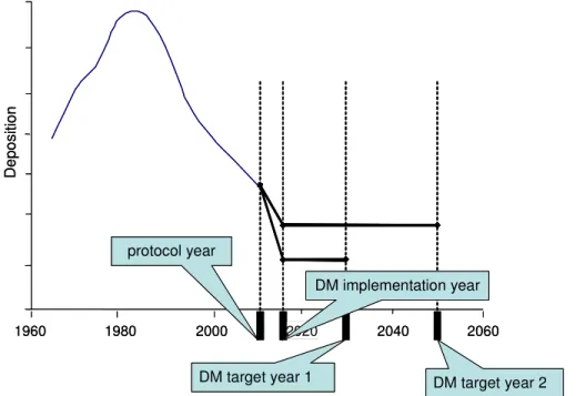
Important dynamic modelling results for possible use by the TFIAM are so-called target loads. A target load is the deposition (path) which ensures recovery by having the prescribed chemical (or, ideally, biological) criterion (e.g., the Al:Bc ratio) be met in a given year and maintained thereafter. The variety of deposition paths to reach a target load is numerous. We restrict to deposition pathways that are characterised by three numbers (years): (i) the protocol year, (ii) the implementation year, and (iii) the target year (see Figure 1-1). The protocol year for dynamic modelling is the year up to which the deposition path is assumed to be known and cannot be changed any more. This can be the present year or a year in the (near) future, for which emission reductions are already agreed. As protocol year countries were requested to use 2010, the year for which the Gothenburg Protocol and the EU NEC Directive are expected to be in place. The implementation year for dynamic modelling is the year in which all reduction measures to reach the final deposition (the target load) are assumed to be implemented. Between the protocol year and the implementation year deposition are assumed to change linearly. After consultation with the chairmen of the ICP M&M, the WGE, the Working

(10)

Group on Strategies and Review (WGSR) and other Convention representatives, 2015 was chosen as a preliminary implementation year. The target year for dynamic modelling is the year in which the chemical criterion (e.g., the Al:Bc ratio) is met (for the first time). Countries were requested to submit target loads for the years 2030, 2050 and 2100.

1960 1980 2000 2020 2040 2060

protocol year

DM implementation year

DM target year 1 _{DM target year 2}

D ep ositi on 1960 1980 2000 2020 2040 2060 protocol year DM implementation year

DM target year 1 _{DM target year 2}

D

ep

ositi

on

Figure 1-1. Schematic representation of deposition paths leading to target loads by dynamic modelling (DM), characterised by three key years. (i) The year up to which the (historic) deposition is fixed (protocol year); (ii) the year in which the emission reductions leading to a target load are implemented (DM implementation year); and (iii) the years in which the chemical criterion is to be achieved (DM target years)

In addition to information on target loads and target years, NFCs were also requested to ensure consistency between critical loads and dynamic modelling. This implies that each record in the critical load database should contain data that can be used to compute critical loads and to run the dynamic model. However, to maintain important statistical information on the (distribution of) sensitivity of ecosystems within an EMEP grid cell, NFCs were requested not to leave out records where only critical loads data were available. Information on the deposition history was available from EMEP Lagrangian modelling results (Schöpp et al., 2003; EMEP, 1998). Results of the call for data were

presented at the 14th_{CCE workshop and 20}th_{Task Force Meeting of the ICP M&M. These meetings}

were held from 24 to 29 May 2004 at the International Institute of Applied Systems Analysis (IIASA/CIAM) in Laxenburg upon invitation by the Federal Ministry of the Environment of Austria.

1.3 Results of the call for data

Sixteen countries submitted updated data on critical loads of acidity and of nutrient N. As approved under the Convention, the European background database is used to compute and map critical loads for ecosystems in countries that never submitted data. For countries who submitted data in one of the earlier calls for data, the latest available submission of critical loads was used.

The critical loads consist of four basic variables which were asked to be submitted and which were used to support the Gothenburg Protocol. These variables are the basis for the maps used in the effect modules of the European integrated assessment modelling effort: (a) the maximum allowable

deposition of S, CLmax(S), i.e. the highest deposition of S which does not lead to ‘harmful effects’ in

(11)

sufficient nitrogen for plant uptake including nitrogen immobilisation (c) the maximum

‘harmless’acidifying deposition of N, CLmax(N), in the case of zero sulphur deposition, and (d) the

critical load of nutrient N, CLnut(N), preventing eutrophication of ecosystems.

Eleven countries also submitted the requested dynamic modelling results. Switzerland reported that it needed more time to prepare a representative set of dynamic modelling data. Belgium, the Czech Republic, Denmark, and Slovakia indicated that they could not finalise their response to the call for data in time. Norway and Sweden noted the preliminary nature of their submission. Many countries

indicated at the 14th_{CCE workshop and 20}th_{Task Force of the ICP Modelling and Mapping that their}

submission of dynamic modelling data should be used in integrated assessment for testing purposes only, while emphasising that a follow-up call for data at the end of 2004 should be considered. Dynamic modelling results submitted in this call are likely to change when depositions of acidifying compounds

computed with the Unified Model on a 50x50 km2_{can become available for dynamic modelling instead}

of depositions computed with the EMEP Lagrangian model on 150x150 km2_{grid cells which were used}

in this round.

Table 1-1. Overview of the response to the call for, and status of, European critical loads on acidification and

eutrophication including preliminary dynamic modelling results#

colnr. 1 CLaci TLFs 2 2030 3 2030 4 2030 5 2050 6 2050 7 2050 8 CLnut 9 Km2 _% _{TL=PL TL<CL} _n.f. _{TL=PL TL<CL} _n.f. _km2 AT* 37572 99.9 96.4 3.4 0.0 96.6 3.3 0.0 37572 BE 7282 - - - 7282 BG* 48345 0.0 0.0 0.0 0.0 0.0 0.0 0.0 48345 BY* 103366 - - - 103366 CH* 11238 - - - 21866 CY* 4534 - - - 4534 CZ 18272 - - - 18272 DE* 105745 61.8 48.1 12.2 1.5 48.3 12.3 1.2 105745 DK* 3149 - - - 3149 EE 21450 - - - 22411 ES 85225 - - - 85225 FI* 266830 - - - 240403 FR* 180102 100.0 97.4 2.6 0.0 97.5 2.5 0.0 180102 GB* 77674 0.8 0.7 0.1 0.0 0.5 0.2 0.0 74206 HR 6931 - - - 7009 HU* 10448 100.0 100.0 0.0 0.0 100.0 0.0 0.0 10448 IE 8936 - - - 8936 IT* 119854 100.0 100.0 0.0 0.0 100.0 0.0 0.0 119854 MD 11985 - - - 11985 NL* 7583 100.0 64.5 13.5 22.0 64.5 13.6 21.9 4623 NO* 453087 19.9 11.2 8.4 0.3 11.2 8.4 0.3 226631 PL* 88383 100.0 88.1 11.9 0.0 88.2 11.8 0.0 88383 RU 3517136 - - - 3517136 SE* 395101 63.8 52.7 8.7 2.4 53.1 8.8 1.9 182223 SK 19227 - - - 19227 * _{Revised data submitted in 2004;}

#_{TLFs = Target load functions; TL = Target load; PL = Present load; CL = Claci km}2_{= The ecosystem area for}

which critical loads of acidification are available; n.f. = Not feasible; Clnut km2_{= The ecosystem area for}

which critical loads of nutrient N are available; critical load calculation and mapping methods are summarised in Hettelingh et al. (2003).

Results are summarised in Table 1-1, which gives an overview of the ecosystem area for each country (column 1) for which critical loads of acidity (column 2) and critical loads of nutrient nitrogen (last column) are available. The latest available submission of critical loads was used for countries who did not

(12)

submit data in 2004. Information is also provided (column 3) on the percentage of a country’s ecosystem area for which dynamic modelling results (target loads) have been submitted. Eight out of eleven countries were able to compute target loads for 100% of the ecosystem area. For other countries a subset of the ecosystem area was used for dynamic modelling. Next, Table 1-1 shows the percentage of the ecosystem area for which the chemical criterion is no longer violated when the emissions of the protocol year are kept constant between 2010 and 2030 (column 4) and 2050 (column 7). In principle this percentage should be larger in 2050 than in 2030. A relatively low percentage of the ecosystem area could recover with target loads lower than critical loads in 2030 (column 5) or 2050 (column 8). The percentage of the ecosystem area where submitted target loads for 2030 and 2050 are infeasible are provided in columns 6 and 9, respectively. The percentage of ecosystems for which target loads are infeasible is high in the Netherlands in comparison to other countries because tentative use was made of an indicator on nitrogen availability and soil pH to describe the change (recovery) of plant species composition (biodiversity). Other countries do not (yet) include biodiversity in their assessments. When applications are restricted to criteria described in the Mapping Manual, such as the calcium-aluminium ratio, percentages similar to other countries are obtained for the share of infeasible areas. Figure 1-2 shows the EMEP grid cells for which target loads were submitted. Target loads turn out to be available in most of the European EMEP grid cells which are exceeded (see Figure 1-6). For countries that never submitted critical loads, the background database could also be used to compute target load values which are compatible with the critical loads.

Figure 1-2. EMEP grid cells (red shaded) for which target load values have been submitted by the National Focal Centres of Austria, Bulgaria, France, Germany, Hungary, Italy, the Netherlands, Norway, Poland, Sweden and the United Kingdom.

(13)

1.4 Maps of critical loads

This section contains maps of critical loads for ecosystems within 50×50 km2_{EMEP (EMEP50) grid}

cells. The maps are based on updated national contributions from 16 countries. For other countries the latest data submission was used. For countries that never submitted critical loads data the European background database (Posch et al., 2003) has been used.

Figure 1-3 shows 5th_{and 50}th_{percentile maps of CL}

max(S) and CLnut(N), reflecting deposition values in

grid cells at which 95% and 50% of the ecosystems are protected respectively. In these maps the critical loads of all ecosystems have been combined. The analysis of critical loads required to protect

95% of the ecosystems from acidification reveals that most sensitive areas (CLmax(S) lower than 200

eq ha-1_a-1_{) occur in northern Europe, the east of the United Kingdom, the south west of France and in}

Belarus. To protect 50% of the areas, low critical loads prevail in northern Europe. The difference

between the 5th_{an 50}th_{percentile maps of CL}

nut(N) is illustrated for example in Germany, Moldova,

Poland, Sweden and Russia where the areas in the lowest critical load range (red shaded) are clearly reduced. This is obvious because higher percentiles correspond to higher critical loads that protect a smaller area of ecosystems.

Figure 1-3. The 5th percentiles of the maximum critical loads of sulphur (top left), and of the critical loads of

nutrient nitrogen (top right). The 50th_{percentiles are shown at the bottom left and right, respectively. The maps}

(14)

Figure 1-4 shows analogous maps for CLmax(N) and CLmin(N). Relatively low values of the 5th

percentile CLmax(N), indicating the maximum critical load for nitrogen acidity at zero deposition of

sulphur, occur mostly in the northern regions of Europe (see top left map). Values of the 5th_percentile

CLmin(N) reflecting the lowest acceptable thresholds of nitrogen uptake and immobilisation, tend to be

low in most parts of Europe (top right map).

Figure 1-4. The 5th percentiles of the maximum critical loads of nitrogen (top left), and of the minimum critical

loads of nitrogen (top right), on the EMEP50 grid resolution. The 50th_{percentiles are shown at the bottom left}

and right, respectively.

1.5 Comparison of 2003 and 2004 critical loads

Figure 1-5 provides a comparison of the statistics of the 2003 and 2004 critical load data. The

minimum, 5th_{, 25}th_{, 50}th_{, 75}th_{, 95}th_{percentiles and the maximum of the critical loads of each country}

that submitted data in 2004 are shown in a ‘diamond plot’. Statistics of CLmax(S) are on the left

ranging over an interval of 0 to 4000 eq ha-1 _a-1_{, whereas CL}

nut(N) (right) ranges from 0 to 2000 eq ha-1

a-1_{. The dark blue and turquoise diamonds reflect 2004 and 2003 statistics respectively. A comparison}

between 2003 and 1998 (critical loads used to support the Gothenburg Protocol) can be found in Hettelingh et al. (2003). This year the recently appointed NFC of Cyprus (CY) made a first

submission of critical loads, therefore a comparison with 2003 data is lacking. Compared to 2003 the

median values (shown as vertical line dividing a ‘diamond’) of CLmax(S) increased in Austria (AT),

(15)

Kingdom (GB), Norway (NO) and Poland (PL). For CLnut(N) the median value has increased in

Belarus and decreased in Austria, Germany, France, the Netherlands and Poland. The 5th_{percentile of}

CLnut(N) of 2004 is lower in Austria, Germany, France, The Netherlands and Poland. Changes in the statistics are a result of updates of national critical load databases, details of which are provided in the NFC reports (see Part II).

Figure 1-5. Diamond plot of the minimum, 5th_{, 25}th_{, 50}th_{, 75}th_{, 95}th_{percentiles and maximum critical loads of}

CLmax(S) (left) and CLnut(N) (right) for the national data of 2004 (dark-blue) and 2003 (turquoise), respectively.

The legend shows that 5th_{percentile is indicated by the dot to the left of the diamond and the 95}th_{percentile by}

the dot on the right, while the median is indicated by the vertical line in the diamond.

1.6 Maps of critical load exceedances

Exceedances in this section refer to the ‘average accumulated exceedance’ (AAE). The AAE is the area-weighted average of exceedances (accumulated over all ecosystem points) in a grid cell, and not only the exceedance of the most sensitive ecosystem. An AAE may be computed for all ecosystem categories within a grid cell, but also for one single ecosystem category (such as a forest) in a grid cell for which data points are submitted by an NFC. The European critical load database contains about 1.4 million critical load data points. Maps of AAE provide information about the magnitude of the exceedances (see Posch et al., 2001 for further details). The AAE, for all ecosystems, was used in integrated assessment modelling to support the analysis of emission reduction alternatives.

The analysis in this section focuses on the difference in magnitudes of the AAE for acidity (a) when using acid deposition values computed with two different EMEP models, i.e. the well-known

(16)

Lagrangian model (EMEP, 1998) and the more recent Unified Model (Tarrasón et al., 2003), (b) when

computed in EMEP50 and 150x150 km2_{(EMEP150) grid cells, and (c) when using acid deposition}

values computed on forest ecosystems or as average. Combinations of (a), (b) and (c) are explored as well. The AAE has been computed using critical loads of acidity.

Figure 1-6 shows a sequence of 6 maps of average accumulated exceedance as follows:

1. The top-left AAE map is based on average acid deposition in EMEP150 grid cells with the

Lagrangian model and critical loads of 1998. This AAE map was used in support of the Gothenburg Protocol. The result shows two grid cells on the border of the Netherlands and

Germany, where the AAE exceeds 800 eq ha-1_a-1_{(red shading).}

2. The top-right AAE map is similar to (1), except that the latest critical load database (2004) is

used. The AAE turns out to decrease on the border of Germany and The Netherlands (and in the Etna region) and increase in eastern Germany and Poland.

3. The left-middle AAE map is similar to the map described in (2), i.e. based on Lagrangian average

deposition and 2004 critical loads, on 50x50 km2_{EMEP grid cells. The Lagrangian deposition}

computed as average in a 150x150 km2_{grid cell is applied to the 50x50 km}2_{grid cells inside.}

4. The right-middle map shows the AAE when the Lagrangian deposition used in (3) is replaced by

the grid average acid deposition computed with the Unified Model, (using an average of the 1999 and 2003 meteorology). The 2004 critical load database is used to compute AAE. The use of the Unified Model to compute grid-average depositions turns out to reveal lower AAE magnitudes on the German-Dutch and German-Czech border than when the Lagrangian model is used. However, overall the differences are not striking.

5. The bottom-left map shows the AAE computed with 2004 critical loads using forest–specific

deposition for forests while using the average deposition for non-forest ecosystems. The deposition values are all computed with the Unified Model. Compared to map 4, much higher exceedances occur due to the fact that deposition onto a forest is higher than the average of depositions over various ecosystems within a grid cell. The reason why the deposition to forests is higher than average deposition is due to the ‘roughness’ of forests which ‘catches’ more

pollutants. Therefore, an ecosystem specific AAE is more accurate than the grid average

computed in the past, using the Lagrangian EMEP model. Ideally, depositions would be required for each of the 1.4 million critical load data points submitted by NFCs to further improve the accuracy of AAE.

6. Finally, the bottom-right map is analogous to (5), but now using only the critical loads of forest

ecosystems and forest specific deposition. The difference with map (5) is not significant with respect to the magnitude and regional distribution of the AAE. The reason is that most of the critical loads are computed for forest soils.

(17)

Figure 1-6. Average accumulated Exceedance (AAE) in 2000 using EMEP Lagrangian model average

deposition with 1998 critical loads on 150x150km2_{(top left), idem with 2004 critical loads (top right), idem on}

50x50 km2_{(middle-left), using EMEP-Unified-model average deposition with 2004 critical loads (middle-right),}

idem using EMEP-Unified-model forest-specific deposition and the average deposition for other ecosystems (bottom-left), and finally focussing on forests only (bottom right).

(18)

Table 1-2 lists the results mapped in Figure 1-6 in terms of the percentage of the ecosystem area which is unprotected from acidification. The Table includes also results for 2010 and reflects two European regional breakdowns, i.e. one region covering most of the 49 European Parties to the Convention (‘Europe’) for which deposition and critical loads data are available, and the other mapping the European Union of 25 member states (‘EU25’). Table1-3 is analogous to Table 1-2 showing the percentage of the ecosystem that is unprotected for the risk of excessive nutrient nitrogen deposition.

Table 1-2. Percentage of the ecosystem area for which acidity critical loads are exceeded in 2000 and 2010

according to the emissions ceilings prescribed in the Gothenburg Protocol and NEC directive*

2000 2010

Europe EU25 Europe EU25

Lagrangian model

(1) 1998 critical loads 3.9 8.5 2.3 4.2

(2) 2004 critical loads 6.4 12.2 4.7 8.3

Unified Model & 2004 Crit.loads

(4) grid average deposition 8.2 15.4 5.4 8.7

(5) ecosystem specific deposition 11.0 22.4 8.2 16.0

(6) forests onlya _13.3 _23.7 _10.0 _17.0

*_{Numbers in brackets refer to the explanations of the consecutive maps of Figure 1-6.} a_{numbers refer to % of forest area.}

Compared to the use of the 1998 critical loads database, Table 1-2 shows that the update of the critical loads database in 2004 yields an increase in Europe of ecosystems at risk of acid deposition, as computed with the Lagrangian model both in 2000 (+1.5 percent point) and 2010 (+2.4 percent point). The use of the Unified Model to compute a grid average deposition leads to a further increase of the unprotected ecosystem area in Europe to 8.2% and 5.4% in 2000 and 2010 respectively. When distinguishing between forest specific deposition and other ecosystems (average deposition) then the percentage of unprotected ecosystems in Europe increases further by about 3.0 percent point. Finally it can be seen that 13.3% and 10% of the forest ecosystems is unprotected in Europe in 2000 and 2010 respectively when forest specific deposition (Unified Model) is compared to forest critical loads of acidity. Thus, compared to the area of all ecosystems at risk of average acidification computed in 1998-1999 (3.9% in 2000 and 2.3% in 2010), computations of ecosystem specific acidification now reveals that 11% is unprotected in 2000 which is reduced to 8.2% in 2010.

Table 1-3. Percentage of the ecosystem area for which nutrient nitrogen critical loads are exceeded in 2000 and

2010 according to the emissions ceilings prescribed in the Gothenburg Protocol and NEC Directive.*

2000 2010

Europe EU25 Europe EU25

Lagrangian model

1998 critical loads 26.0 60.7 24.6 54.4

2004 critical loads 24.5 56.0 23.1 49.0

Unified Model & 2004 Crit.loads

grid average deposition 29.2 64.9 28.5 59.2

ecosystem specific deposition 35.1 77.7 34.7 73.0

forests onlya _53.2 _80.9 _52.3 _76.3

*_{Explanations are analogous to Table 1-2.} a_{numbers refer to % of forest area.}

Table 1-3 shows that the area of all ecosystems at risk of average eutrophication computed for 1998 critical loads (26% in 2000 and 24.6% in 2010), increases to 35.1% in 2000 and 34.7% in 2010 when computing ecosystem-specific eutrophication. The use of the critical loads database of 2004 to compute exceedances with Lagrangian-modelled depositions leads to a decreasing percentage of ecosystems at risk, i.e. from 26% to 24.5% in 2000 and from 24.6% to 23.1% in 2010. The use of nitrogen deposition computed with the Unified Model shows that the percentage of unprotected ecosystems increases significantly to 53.2% in 2000 (52.3% in 2010) when focussing on forest soils.

(19)

Note that the area of ecosystems that are unprotected from eutrophication (see Table 1-3) is significantly larger than area which is unprotected from acidification (Table 1-2), both in 2000 and 2010. Finally, also note in Tables 1-2 and 1-3, that the percentage of the unprotected ecosystems in the EU25 is generally higher than in Europe. The reason is that Russia contains a relatively large area of protected ecosystems.

In summary, the increase of the computed risk of acidification can be attributed both to the updated critical loads database as to EMEP computed depositions using the Unified Model. However, the increase of the computed risk of eutrophication is largely due to deposition results generated with the Unified Model. The ability of the Unified EMEP model to compute ecosystem specific depositions improves the quality of the assessment of risks based on critical loads within a single EMEP grid cell. Where in the past only one single average deposition value could be compared to a range of critical loads (for different ecosystem categories) to yield an average risk, now specific risk assessments are possible focussing on an individual ecosystem within an EMEP grid cell. This increases the similarity with findings in the field, where measured deposition has been shown to be higher in forest

ecosystems than outside.

References

EMEP (1998) Transboundary acidifying air pollution in Europe, MSC-W Status Report 1998 – Parts 1 and 2. EMEP/MSC-W Report 1/98, Norwegian Meteorological Institute, Oslo, Norway.

Hettelingh, J-P, Posch M, Slootweg J (2003) Status of European critical loads and dynamic modelling, In: M Posch, J-P Hettelingh, J Slootweg, RJ Downing (eds) Modelling and mapping of critical thresholds in Europe, CCE Status Report, 2003.RIVM Report 259101013, RIVM, Bilthoven, the Netherlands, pp.1-10.

Posch M, Hettelingh J-P, Slootweg J (eds) (2003) Manual for dynamic modelling of soil response to atmospheric deposition. Coordination Center for Effects, RIVM Report 259101012, Bilthoven, Netherlands, 71 pp. www.rivm.nl/cce

Posch M, Hettelingh J-P, De Smet PAM (2001) Characterization of critical load exceedances in Europe. Water Air

Soil Pollut. 130: 1139-1144.

Schöpp W, Posch M, Mylona S, Johansson M (2003) Long-term development of acid deposition (1880–2030) in sensitive freshwater regions in Europe. Hydrol Earth Syst Sci 7: 436–446.

Tarrasón L, Jonson JE, Fagerli H, Benedictow A, Wind P, Simpson D, Klein H (2003) Transboundary acidification eutrophication and ground level ozone in Europe, Part III: Source-receptor relationships. EMEP Report 1/2003, Norwegian Meteorological Institute, Oslo, Norway.

(20)

(21)

2 Summary of National Critical Loads Data

Jaap Slootweg, Maximilian Posch and Jean-Paul Hettelingh

2.1 Introduction

The 1998 European critical loads database was used to support the negotiations of the effects-based Gothenburg Protocol of the 1979 Convention on Long-range Transboundary Air Pollution. Since then progress has been made in the work of the scientific community supporting the effects-related work in relation to critical loads and dynamic modelling. Members of the Working Group on Effects (WGE) welcomed the progress achieved in the application of dynamic modelling and the steps taken to link

dynamic modelling to integrated assessment. Consequently, the WGE in its 22th_{session invited the}

CCE ‘to issue a call for data on critical loads and dynamic modelling data in autumn 2003.’ To apply dynamic modelling data to integrated assessment, the CCE also requested target loads in addition to critical loads. A target load is the deposition for which a pre-defined chemical (or

biological) status is reached in the target year, and maintained (or improved) thereafter. To ensure the robustness of integrated assessment updated critical loads, consistent with target loads, are necessary. To demonstrate the pathways of recovery of ecosystems with decreasing acidifying depositions the CCE also requested in this call the value of the applied criterion in the target years 2030, 2050 and 2100.

This chapter reports on the steady state results (critical loads and parameters) of the call for data issued in December 2003 with the deadline of 31 March 2004. The results and parameters related to dynamic modelling are described in Chapter 3.

2.2 Requested variables

A complete submission for this call consisted of

(1) Updated critical loads

(2) Target load functions for the target years 2030, 2050 and 2100

(3) Value of the applied criterion in the target years when running the dynamic model with the

2010 (Gothenburg) depositions kept constant afterwards.

(4) Input variables to allow consistency checks and inter-country comparisons

Previous calls demanded a single table of ecosystems with its properties, but the extended scope of this year’s call brought about the use of related tables which contained respectively:

- input variables and critical loads ‘Table 1’

- target load functions ‘Table 2’

- values of the applied criterion in target years ‘Table 3’

To simplify the inclusion of dynamic modelling results for aquatic ecosystems, a specific format was adopted with relevant input variables ‘Table 4’. A list of all four Tables, with their variable names, units and a description as send to all National Focal Centres can be found in Annex I.

(22)

2.3 National responses

Cyprus submitted critical loads for the first time, bringing the number of National Focal Centres (NFCs) to 25. The CCE had communications (nearly 500 e-mails) with 23 countries, of which 16 submitted data. From these 11 countries also submitted results of dynamic modelling. Switzerland indicated to have calculated target loads, but needed further investigation. Belgium, the Czech Rebublic, Denmark, Slovakia and Switzerland have indicated to be working on dynamic modelling, but need more time. Sweden submitted target loads, but stated that the critical load data of 2003 is still valid, and dynamic modelling results are not to be used for policy purposes. An overview of the national submissions is given in Table 2-1.

Table 2-1. National responses to the call for critical loads and dynamic modelling results.

Country Code Critical loads

data Dynamic modelling results

Remarks

(DM = Dynamic Modelling.)

Austria AT X X

Belarus BY X -

Bulgaria BG X All sites safe

Cyprus CY X -

Denmark DK X -

Finland FI X -

France FR X X

Germany DE X X

Hungary HU X All sites safe

Italy IT X All sites safe

Netherlands NL X X

Norway NO X X

Poland PL X X

Sweden SE X X DM not for policy purposes

Switzerland CH X - ‘More time needed’

United Kingdom GB X X

Total NFCs 16 11

2.4 Types, numbers and areas of the national submissions

All 16 submissions adopted the EUropean Nature Information System (EUNIS) to classify the ecosystem types, and some used a very detailed level. These levels are truncated to a maximum of 2 characters. The figures in this chapter show aggregated categories of the submitted ecosystem types to EUNIS level 1, or grouped further into the main categories listed in the first column of Table 2-2.

(23)

Table 2-2. Types of ecosystems for different levels, as used in this report.

Main

categories EUNIS Level 1 EUNIS code EUNIS description

Forest Forest G Woodland and forest habitats and other wooded land

G1 Broadleaved deciduous woodland

G2 Broadleaved evergreen woodland

G3 Coniferous woodland

G4 Mixed deciduous and coniferous woodland Vegetation Grassland E Grassland and tall forb habitats

E1 Dry grasslands

E2 Mesic grasslands

E3 Seasonally wet and wet grasslands E4 Alpine and sub alpine grasslands Shrubs F Heath land, scrub and tundra habitats

F1 Tundra

F2 Arctic, alpine and sub alpine scrub habitats

F4 Temperate shrub heath land

F5 Maquis, matorral and thermo-Mediterranean brushes

F7 Spiny Mediterranean heaths

F9 Riverine and fen scrubs

Wetlands D Mire, bog and fen habitats

D1 Raised and blanket bogs

D2 Valley mires, poor fens and transition mires

D4 Base-rich fens

D5 Sedge and reed beds, normally without free-standing water D6 Inland saline and brackish marshes and reed beds

Other A2 Littoral sediments

B1 Coastal dune and sand habitats

B2 Coastal shingle habitats

C3 Littoral zone of inland surface water bodies

Y Undefined

Water Water C Inland surface water habitats

C1 Surface standing waters

C2 Surface running waters

Table 2-3 lists the areas (in km2_{) and the number of submitted ecosystems, indicating the resolution}

each country uses for its calculations.

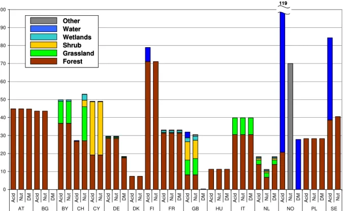
Figure 2-1 shows the percentage of the total country area for which critical loads have been submitted, separately for acidification, eutrophication, and ecosystems for which dynamic modelling has been performed. Most countries that submitted dynamic modelling results were able to do so for a part of the total data set. Norway and the United Kingdom submitted target loads for aquatic ecosystems. Forest is the dominant ecosystem considered in most of Europe, but also waters (mainly in the Northern part of Europe), grassland, shrubs and wetlands are considered. The United Kingdom, Norway and Sweden have a separate dataset for aquatic ecosystems for which DM results have been submitted. (Swedish DM data are not shown in Figure 2-1). The forested area of Norway can be part of the catchment area of the submitted rivers and lakes, counting areas twice (resulting in a coverage of 119% of the total country area).

(24)

0 10 20 30 40 50 60 70 80 90 100 A ci d N ut D M A ci d N ut D M A ci d N ut A ci d N ut A ci d N ut A ci d N ut D M A ci d N ut A ci d N ut A ci d N ut D M A ci d N ut D M A ci d N ut D M A ci d N ut D M A ci d N ut D M A ci d N ut D M A ci d N ut D M A ci d N ut AT BG BY CH CY DE DK FI FR GB HU IT NL NO PL SE

Figure 2-1. National distribution of ecosystem types (% of total country area) for critical loads for acidification (Acid) eutriphication (Nut) and results of dynamic modelling (DM).

Table 2-3. Number of ecosystems and areas per national contribution.

Acid CLs Nutrient CLs Dyn.mod. results

Country Total Country

Area EUNIS lev.1 # ecosyst (kmArea 2₎ # ecosyst _(kmArea 2₎ # ecosyst _(kmArea 2₎

Austria 83858 Forest 489 37,572 489 37,572 487 37,521 Belarus 207595 Forest 6,917 76,316 6,917 76,316 Grassland 1,542 25,302 1,542 25,302 Wetlands 145 1,746 145 1,746 total 8,604 103,364 8,604 103,364 Bulgaria 110994 Forest 88 48,345 88 48,345 4 0 Cyprus 9251 Forest 7,099 1,775 7,099 1,775 Shrub 10,951 2,738 10,951 2,738 Other 87 22 87 22 total 18,137 4,535 18,137 4,535 Denmark 43094 Forest 9,758 3,149 9,758 3,149 Finland 338144 Forest 3,079 240,379 3,083 240,403 Water 1,450 26,426 total 4,529 266,805 3,083 240,403 France 543965 Forest 3,840 170,657 3,840 170,657 3,840 170,657 Grassland 81 1,580 81 1,580 81 1,580 Wetlands 67 5,123 67 5,123 67 5,123 Other 156 2,741 156 2,741 156 2,741 total 4,144 180,101 4,144 180,101 4,144 180,101 Other Water Wetlands Shrub Grassland Forest Other Water Wetlands Shrub Grassland Forest Other Water Wetlands Shrub Grassland Forest 119 119

(25)

Germany 357022 Forest 406,750 101,688 406,750 101,688 251,163 62,791 Grassland 7,170 1,793 7,170 1,793 5,532 1,383 Shrub 2,703 676 2,703 676 382 96 Wetlands 5,579 1,395 5,579 1,395 4,046 1,012 Other 779 195 779 195 200 50 total 422,981 105,747 422,981 105,747 261,323 65,332 Hungary 93030 Forest 6,615 10,460 6,615 10,460 6,615 10,460 Italy 301336 Forest 338 91,910 338 91,910 338 91,910 Grassland 164 27,943 164 27,943 164 27,943 total 502 119,853 502 119,853 502 119,853 Netherlands 41526 Forest 35,375 5,786 17,060 2,827 35,375 5,786 Grassland 8,055 1,027 8,055 1,027 8,055 1,027 Shrub 1,717 343 1,717 343 1,717 343 Wetlands 1,540 230 1,540 230 1,539 230 Other 649 197 649 197 649 197 total 47,336 7,583 29,021 4,624 47,335 7,583 Norway 323759 Forest 662 67,011 Water 2,435 386,077 121 90,115 Other 1,610 226,631 total 3,097 453,088 1,610 226,631 121 90,115 Poland 312685 Forest 88,382 88,382 88,382 88,382 88,382 88,382 Water 1 1 1 1 total 88,383 88,383 88,383 88,383 88,382 88,382 243307 Forest 150,208 19,748 151,815 19,896 United Kingdom _Grassland _99,451 _20,010 _119,062 _21,897 Shrub 78,550 24,669 78,985 24,785 Wetlands 18,682 5,455 19,079 5,506 Water 1,717 7,790 109 599 Other 10,299 2,119 total 348,608 77,672 379,240 74,203 109 599 Switzerland 41285 Forest 691 11,056 1,456 11,191 Grassland 7,777 7,777 Shrub 1,512 1,512 Wetlands 1,348 1,348 Water 101 182 38 38 total 792 11,238 12,131 21,866 Sweden 449964 Forest 1,764 173,759 1,863 182,223 Water 2,887 205,502 total 4,651 379,261 1,863 182,223

2.5 National critical loads and input variables

This section shows the critical loads and most important related variables of the national

contributions. The characteristics can often be explained by studying the national reports, in Part II of this report.

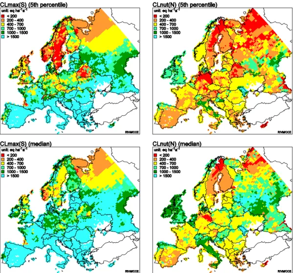
Figure 2-5 show the 5th_{percentile and median values for the critical loads for sulphur and nutrient}

nitrogen on EMEP50 grid for the countries that submitted data this year. Compared to last years

results the updates in critical loads show only minor changes for CLmax(S) (see Posch et al., 2003.)

Belarus has extended the area for which they made their calculations to the whole of the country. Germany and Poland appear a little less sensitive.

(26)

In comparison with 2003 the updated CLnut(N) for the Netherlands is more in line with its neighbouring countries. Germany is more sensitive than earlier. (See Posch et al., 2003).

unit: eq ha-1_a-1 < 200 200 - 400 400 - 700 700 - 1000 1000 - 1500 > 1500 CLmax(S) (5th percentile) CCE unit: eq ha-1_a-1 < 200 200 - 400 400 - 700 700 - 1000 1000 - 1500 > 1500 CLmax(S) (median) CCE unit: eq ha-1_a-1 < 200 200 - 400 400 - 700 700 - 1000 1000 - 1500 > 1500 CLnut(N) (5th percentile) CCE unit: eq ha-1_a-1 < 200 200 - 400 400 - 700 700 - 1000 1000 - 1500 > 1500 CLnut(N) (median) CCE

Figure 2-2. The 5th_{percentile (left) and median (right) EMEP50 grid values of the maximum critical loads of}

sulphur (top) and the critical loads of nutrient nitrogen (bottom).

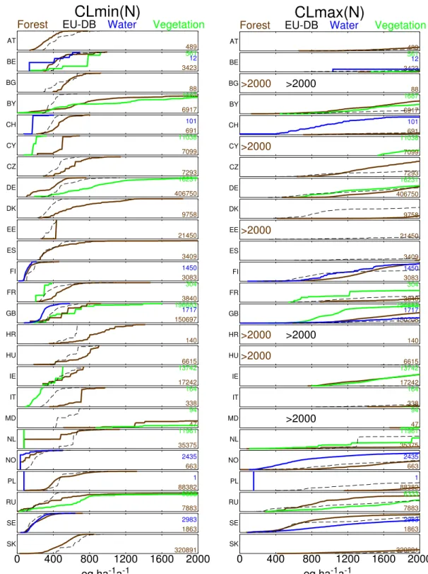
The complete distributions of the national critical loads, CLmax(S), CLmin(N), CLmax(N) and CLnut(N) are

plotted in Figure 2-3 and Figure 2-4 in a cumulative distribution function (cdf) for all countries that submitted data for this or previous calls. The cdfs show the cumulated area of ecosystems as a function of the variable, normalised to 100% (no vertical scale is plotted in the cdf-graphs). The thin black dotted line (‘EU-DB’) represents the cdf of the respective variable from the European

background database, which contains data for forest soils only (see Chapter 3). The ecosystem types are the aggregated classes from the first column of Table 2-2. The number of ecosystems is also given for every cdf, except for the cdfs of background database.

(27)

CLmaxS

Forest EU-DB Water Vegetation

AT BE BG BY CH CY CZ DE DK EE ES FI FR GB HR HU IE IT MD NL NO PL RU SE SK 0 400 800 1200 1600 2000 eq ha-1a-1 489 3423 561₁₂ >2000 ₈₈ 6917 1687 691 101 11038 7099 7293 16231 406750 9758 21450 3409 3083 1450 3840 304 196683 150208 1717 140 >2000 6615 17242 13742 164 338 47 94 >2000 35375 11961 663 2435 88382 1 7883 6333 1863 2983 320891

CLnut(N)

AT BE BG BY CH CY CZ DE DK EE ES FI FR GB HR HU IE IT MD NL NO PL RU SE SK 0 400 800 1200 1600 2000 eq ha-1a-1 489 3423 561 >2000 12 88 6917 1687 1456 10637 38 11038 7099 7293 16231 406750 9758 21450 961 3409 3083 3840 304 227425 151815 144 6615 17242 13742 164 338 47 94 11961 17060 1610 88382 1 7883 6333 1863 320891

Figure 2-3. The cumulative distribution functions (cdfs) of maximum critical load of sulphur (left) and the critical load of nutrient nitrogen (right) for forest water and vegetation, and for the European background database (‘EU-DB’)

(28)

CLmin(N)

AT BE BG BY CH CY CZ DE DK EE ES FI FR GB HR HU IE IT MD NL NO PL RU SE SK 0 400 800 1200 1600 2000 eq ha-1a-1 489 3423 561₁₂ 88 6917 1687 691 101 11038 7099 7293 16231 406750 9758 21450 3409 3083 1450 3840 304 196683 150697 1717 140 6615 17242 13742 164 338 47 94 35375 11961 663 2435 88382 1 7883 6333 1863 2983 320891

CLmax(N)

AT BE BG BY CH CY CZ DE DK EE ES FI FR GB HR HU IE IT MD NL NO PL RU SE SK 0 400 800 1200 1600 2000 eq ha-1a-1 489 3423 561₁₂ >2000 >2000 ₈₈ 6917 1687 691 101 11038 >2000 ₇₀₉₉ 7293 16231 406750 9758 >2000 ₂₁₄₅₀ 3409 3083 1450 3840 304 196683 150208 1717 >2000 >2000 ₁₄₀ >2000 ₆₆₁₅ 17242 13742 164 338 47 94 >2000 35375 11961 663 2435 88382 1 7883 6333 1863 2983 320891

Figure 2-4. The cdfs of minimum (left) and maximum (right) critical load of nitrogen forest, water and vegetation, and for the European background database.

For most of Europe CLmax(N) is much larger then CLnut(N). This means that with relatively low

depositions of sulphur eutrophication will occur more likely than acidification.

The CCE requested most of the variables that are needed to compute the critical loads. A selection (combination) of the distributions of these variables is plotted in the next graphs, to demonstrate

(29)

characteristics of the national submissions. The graphs will only show the 16 countries that submitted data for this call.

Figure 2-5 shows the amount of water percolating through the root zone (Qle) and the denitrification

fraction (fde). Countries can either assume a fraction to be denitrified (fde) or a fixed amount (Nde). The

choice they made can be derived from the presence of the relevant cdf in the graph for fde. Nde is not

shown in this report, but values are below 250 eq ha-1_a-1_{for most ecosystems. Well-aerated soils will}

have lower denitrification. Ecosystems with a high flow of water are not necessarily wet, and

therefore can have low denitrification, as indicated by the differences in distributions of Qle and fde for

several countries.

Q

_le

Forest EU-DB Water Vegetation AT BG BY CH CY DE DK FI FR GB HU IT NL NO PL SE 0 200 400 600 800 1000 mm a-1 489 88 6917 1687 691 11038 7099 16231 406750 3083 3840 304 217015 151280 6615 164 338 35375 11961 88382 1863 2983

f

_de

AT BG BY CH DE DK FI FR GB HU IT NL NO PL SE 0 1 -489 4 691 16231 406750 3083 3840 304 6615 164 338 35375 11961 663 2304 88382

Figure 2-5. The cdfs of the amount of water percolating through the root zone (Qle, left) and the fraction of

nitrogen denitrified in the soil (fde, right)

In the Simple Mass Balance (SMB) model nitrogen leaves the system by denitrification, immobilisation in the soil, net uptake by harvesting and leaching. The long-term acceptable immobilisation and the acceptable leaching of nitrogen are shown in Figure 2-6. The background

database uses the constant value of 1 kgN ha-1_a-1_{for immobilisation, as recommended in the Mapping}

(30)

Acceptable N immobilisation

Forest EU-DB Water Vegetation AT BG BY CH DE DK FI FR GB HU IT NL NO PL SE 0 100 200 300 400 500 eq ha-1a-1 489 88 691 16231 406750 9758 3083 1450 3840 304 196665 150697 1717 6615 164 338 35375 11961 663 2395 88382 1863 2983 accept. N leaching Forest EU-DB Vegetation AT BG BY CH CY DE DK FI FR GB HU IT NL NO PL SE 0 100 200 300 400 500 eq ha-1a-1 489 86 691 11038 7099 16231 406750 9758 3083 3840 304 113752 6615 164 338 88382

Figure 2-6. The cdfs of the acceptable amount of nitrogen immobilised in the soil (left) and the acceptable amount of leaching nitrogen.

0 400 800 1200 1600 N uptake (eq ha -1a -1)

AT: 489 sites BG: 88 sites BY: 6917 sites CH: 691 sites

0 400 800 1200 1600 N uptake (eq ha -1a -1)

CY: 7099 sites DE:406750 sites DK: 9757 sites FI: 3083 sites

0 400 800 1200 1600 N uptake (eq ha -1a -1)

FR: 3840 sites GB:151280 sites HU: 6605 sites IT: 338 sites

0 400 800 1200 1600 0 400 800 1200 1600 Bc uptake (eq ha-1_a-1₎ N uptake (eq ha -1a -1) NL: 35375 sites 0 400 800 1200 1600 Bc uptake (eq ha-1_a-1₎ NO: 663 sites 0 400 800 1200 1600 Bc uptake (eq ha-1_a-1₎ PL: 88382 sites 0 400 800 1200 1600 Bc uptake (eq ha-1_a-1₎ SE: 1863 sites

(31)

Figure 2-7 shows the correlation between nitrogen and base cation uptake for forests. The green line gives the ratio for spruce when only stems are harvested. The calculation of this ratio is based on the mean values of element content in stems according to Jacobsen et al. (2002) also listed in Table 5.8 of the Mapping Manual (UBA, 2004).

In previous calls for data the CCE requested base cation weathering and sea salt corrected base cation deposition, but this call asked for the individual ions. The reason is to improve the understanding of the manner in which countries compile the base cation deposition. Figure 2-8 show total base cation weathering and the sea salt corrected base cation deposition. For countries with missing values for the individual ions, it was assumed calcium was used for the total base cation amount, and sea salt correction already applied for the deposition.

Ca+Mg+K+Na weathering Forest EU-DB Vegetation AT BG BY CH CY DE DK FI FR GB HU IT NL NO PL SE 0 400 800 1200 1600 2000 eq ha-1_a-1 489 88 6917 1687 691 11038 7099 16231 406750 9758 3083 3840 304 196665 150210 6615 164 338 35320 11585 663 88382 1863 BC* deposition Forest EU-DB Water Vegetation AT BG BY CH CY DE DK FI FR GB HU IT NL NO PL SE 0 400 800 1200 1600 2000 eq ha-1_a-1 489 88 6690 1619 691 101 11038 7099 16231 406750 9758 3083 1450 3840 304 217066 151275 109 6615 164 338 35375 11961 91 88382 1863 2983

Figure 2-8. The cdfs of base cation weathering (left) and sea salt corrected base cation deposition(right).

In the simplest case, the equilibrium between Al and H in the soil solution can be described by the gibbsite equilibrium. However, in the latest version of the Mapping Manual a more general

(empirical) relationship has been proposed, i.e. [Al] = KAlox[H]expAl, which for expAl=3, includes the

gibbsite equilibrium. In Figure 2-9 the relationship between the logarithm of KAlox and the exponent

expAl is depicted for the NFC data as black dots; and the crosses are from measurements at about 120 European Forest Intensive Monitoring sites (De Vries et al., 2003). Figure 2-9 shows that there is a

strong correlation between log10KAlox and expAl, and that the data used by the NFCs are fairly much in

line with the European observational data. Actually, the majority of the countries (AT, DE, FR, GB,

IT) use the gibbsite equilibrium (expAl=3) with log10KAlox=8, here highlighted as the intersection point

of the axes.

The latest additions to the Simple Mass Balance (SMB) method, as described in the Mapping Manual,

are bicarbonate leaching and the inclusion of the dissociation of organic acids. The partial CO2

pressure in the soil (pCO2) is in equilibrium with the concentration of bicarbonate in the soil solution

according to Henry’s law. The unit used for pCO2 is multiples of the partial pressure in air, which is

(32)

-6 -3 0 3 6 9 12 -1 0 1 2 3 4 log10KAlox expAl

Figure 2-9. The logarithm of KAlox versus the exponent expAl describing the Al-H equilibrium. The black dots

are the data from the NFCs, whereas the crosses are derived from measurements at about 120 Forest Intensive Monitoring sites (De Vries et al., 2003). Data lying on the horizontal axis indicate the use of a gibbsite equilibrium (expAl=3).

conc. organic acids

Forest EU-DB Water Vegetation AT BG BY CH DE DK FI FR GB HU IT NL NO PL SE 0 0.05 0.10 0.15 0.20 0.25 eq m-3 489 16231 406750 3840 304 6615 35375 11961 88382 1

part. CO

2

pressure

Forest EU-DB Vegetation AT BG BY CH DE DK FI FR GB HU IT NL NO PL SE 0 8 16 24 32 40 -489 4 16231 406750 3840 304 6615 164 338 35375 11961 88382

Figure 2-10. The cdfs of the concentration of the organic acids (left) and the multiples of partial CO2 pressure

expressed as multiples of the partial pressure of CO2 in the air (right).

Organic acids, if present, could be considered part of the charge balance of the ions in the soil

(33)

(cOrgacids). More details on these extensions of the SMB-method can be found in the Mapping Manual. A few countries adapted to these enhancements, as can be seen in Fig. 2-10.

The background database uses fixed values (cOrgacids = 0.05 eq m-3_{, factor pCO}

2 = 15).

Different chemical criteria are used as limits to protect ecosystems, and for some different critical values apply. Several countries use for certain types of ecosystems combination of criteria, e.g. Bulgaria uses pH and Bc:Al, Germany uses pH and base saturation and the Netherlands use

combinations of Bc:Al, nitrogen availability, base saturation and pH, because it includes biodiversity as endpoint. The criterion used by the countries is listed in Table 2-4 together with ranges for their critical values used.

Table 2-4. Criteria used by the NFCs for ecosystem types as percentages of the total ecosystem numbers.

Al:Bc*) [Al] bsat pH Bc:H ANC other unknown

(range of critical value) 0.5 – 1.7 0.2 eq/m3 _{56-83% 3.8 – 6.2 0.2 – 1.2} 0 – 18 _eq/m3

Country

code Ecosystem type

AT Forest 100 BG Forest 0 0 0 0 0 0 100 BY Forest 100 Vegetation 100 CH Forest 0 0 0 0 0 0 0 100 Vegetation 0 0 0 0 0 0 0 100 Water 0 0 0 0 0 83 0 17 CY Forest 26 74 Vegetation 6 94 DE Forest 18 0 0 44 2 0 37 0 Vegetation 8 0 0 39 23 0 30 0 DK Forest 100 FI Forest 100 0 0 0 0 0 0 0 Water 0 0 0 0 0 100 0 0 FR Forest 83 17 Vegetation 43 57 GB Forest 0 0 0 6 0 0 76 18 Vegetation 0 0 0 0 0 92 0 8 Water 0 0 0 0 0 100 0 0 HU Forest 100 IT Forest 100 0 0 0 0 0 0 0 Vegetation 100 0 0 0 0 0 0 0 NL Forest 49 51 Vegetation 100 NO Forest 0 0 0 0 0 0 0 100 Vegetation 0 0 0 0 0 0 0 100 Water 0 0 0 0 0 25 0 75 PL Forest 100 Water 100 SE Forest 0 0 0 0 0 0 0 100 Water 0 0 0 0 0 0 0 100

*The criterion Bc:Al has been converted to Al:Bc.

It is important that conclusions of integrated assessment based on dynamic modelling are in line with the conclusions based the mapping of critical loads, i.e. that steady state mass balance results are consistent with result of dynamic modelling. The overall distribution of critical loads (by conventional methods and data sets) should therefore be similar to the distribution of critical loads that can be achieved by the methods and data set used in dynamic modelling. In Figure 2-11 the distributions of the maximum critical loads for sulphur and the critical load for nutrient nitrogen are plotted for the whole of the national data sets and the subsets used for dynamic modelling for both terrestrial and aquatic ecosystems. Most deviations are in countries which did dynamic modelling for a specific subset (mostly aquatic ecosystems) of which sufficient data were available.

(34)

CLmax(S) DMvsAll

All DM H2O DMH2O

AT BG BY CH CY DE DK FI FR GB HU IT NL NO PL SE 0 400 800 1200 1600 2000 eq ha-1a-1 489 489 >2000 >2000 ₈₈4 8604 691 101 18137 422981 261323 9758 3083 1450 4144 4144 346891 1717109 6615 6615 502 502 47336 47335 2967 131 121 88383 88382 4846506 131 CLmax(N) DMvsAll

All DM H2O DMH2O

AT BG BY CH CY DE DK FI FR GB HU IT NL NO PL SE 0 400 800 1200 1600 2000 eq ha-1a-1 489 489 >2000 >2000 ₈₈4 8604 691 101 18137 422981 261323 9758 3083 1450 4144 4144 346891 1717109 >2000 >2000 ₆₆₁₅6615 502 502 47336 47335 2967 131 121 88383 88382 4846506 131

Figure 2-11. The maximum critical loads of sulphur (right) and nitrogen (left) for all terrestrial ecosystems (black line), all aquatic ecosystems (dark blue line), and for ecosystems for which dynamic modelling was applied, also split into terrestrial (brownish dashed line) and aquatic (light blue dashed line).

2.6 Conclusions and recommendations

Of the now 25 National Focal Centres, 16 submitted updated critical loads. Critical loads have been updated slightly, the main updates related to the critical load for nutrient nitrogen. Although in many cases the critical loads for forest are higher then for other ecosystem types, especially for low critical loads, forest is still the dominant ecosystem type considered. Regarding aquatic ecosystems an increasing number of ecosystems is considered for dynamic modelling.

With relatively low depositions of sulphur, damage due to eutrophication will be more likely than by acidification. Considering the current trends in sulphur and nitrogen emissions, increasing attention is needed for dynamic modelling of (nutrient) nitrogen.

References

De Vries W, Reinds GJ, Posch M, Sanz MJ, Krause GHM, Calatayud V, Renaud JP, Dupouey JL, Sterba H, Vel EM, Dobbertin M, Gundersen P, Voogd JCH (2003) Intensive monitoring of forest ecosystems in Europe. Technical Report 2003, Forest Intensive Monitoring Coordinating Institute (FIMCI), EC-UNECE, Brussels, Geneva, 161 pp.

Jacobsen C, Rademacher P, Meesenburg H, Meiwes KJ (2002) Element contents in tree compartments – Literature study and data collection (in Germany). Report, Niedersächische Forstliche Versuchsanstalt, Göttingen, Germany, 80 pp.

Posch M, Hettelingh J-P, Slootweg J (eds) (2003) Manual for dynamic modelling of soil response to atmospheric deposition. Coordination Center for Effects, RIVM Report 259101012, Bilthoven, Netherlands. www.rivm.nl/cce

UBA (2004) Manual on Methodologies and Criteria for Modelling and Mapping Critical Loads & Levels and Air Pollution Effects, Risks and Trends, Chapter 5: Mapping Critical Loads. www.icpmapping.org