RIVM report 550015002/2001
Best available practice in life cycle assessment of climate change, stratospheric ozone depletion, photo-oxidant formation, acidification, and eutrophication
Backgrounds on general issues
J. Potting, W. Klöpffer (eds.), J. Seppälä, J. Risbey, S. Meilinger, G. Norris, G.L. Lindfors, M. Goedkoop
This report is prepared by the SETAC Europe Scientific Task Group on Global And RegionaL Impact Categories (SETAC-Europe/STG-GARLIC) that is installed by the 2nd SETAC Europe working group on life cycle impact assessment. The report is published for the account of the Directiorate-General of the National Institute of Public Health and the Environment (RIVM), within the framework of project 550015.
Corresponding address:
Center for Energy and Environmental Studies IVEM University of Groningen Nijenborgh 4 9747 AG Groningen The Netherlands Telephone: 00 31 50 363 46 05 Fax: 00 31 50 363 71 68 Email: J.Potting@fwn.rug.nl
Abstract
This report has been prepared by the SETAC Europe Scientific Task Group on Global And RegionaL Impact Categories (SETAC-Europe/STG-GARLIC) that is installed by the 2nd SETAC Europe working group on life cycle impact assessment (WIA-2). This document is background to a chapter written by the same authors under the title “Climate change, stratospheric ozone depletion, photo-oxidant formation, acidification and eutrophication” in Udo de Haes et al. (2002). The chapter summarises the work of the STG-GARLIC and aims to give a state-of-the-art review of the best available practice(s) regarding category indicators and lists of concomitant characterisation factors for climate change, stratospheric ozone depletion, photo-oxidant formation, acidification, and aquatic and terrestrial eutrophication. Backgrounds on each of the specific impact categories are given in another background report from Klöpffer and Potting (2001).
This background report provides details on a selection of general issues relevant in relation to LCA and characterisation of impact in LCA. The document starts with a short introduction of the LCA methodology and impact assessment in LCA for non LCA-experts. LCA experts, on the other hand, will usually not be familiar in-depth with scientific and political backgrounds of the specific impact categories. A review of this is given. Also the discussion is provided about the issue of the position of the category indicator in the causality chain, and into the related issue of spatial differentiation. These two issues appeared to be one of the core items for SETAC-Europe/STG-GARLIC.
Preface
Methods like integrated modelling of the chain from cause to environmental effect are of growing importance for the support of European Environmental policy. RIVM explores the potential of broadening the basis of such integrated environmental assessment methods with knowledge and conventions applied in Life Cycle Assessment and Substance Flow Analysis in close collaboration with the Center for Environmental Science of the University of Leiden, and the dept. of Science, Technology and Society of Utrecht University, and SETAC1. We are therefore happy to publish this document as a RIVM report.
This document is prepared by SETAC’s Europe Scientific Task Group on Global And RegionaL Impact Categories (SETAC-Europe/STG-GARLIC) that is installed by the second SETAC Europe working group on life cycle impact assessment (WIA-2). This working group has adopted as a priority aim to establish best available practice(s) regarding impact
categories, category indicators, and equivalency factors to be used in impact in Life Cycle Assessment. Scientific Task Groups are formed around groups of impact categories to start this process. SETAC-Europe/STG-GARLIC deals with acidification, aquatic and terrestrial eutrophication, tropospheric ozone formation, stratospheric ozone depletion and climate change.
The ultimate aim is to develop general indicators that integrate environmental side-effects of economic activities, which can be used in decision-making by governments, companies and consumers.
Drs. Rob Maas
(Head of the Environmental Assessment Bureau of RIVM)
Contents
Samenvatting 9
Summary 11
1 Introduction 13
2.1 Introduction 15
2.2 The general framework 15
2.3 The impact assessment phase 19
2.4 Focus of the work 22
3 Sophistication of category indicators 25
3.1 Introduction 25
3.2 Position of category indicators 26
3.2.1 The threshold issue 26
3.2.2 Threshold based category indicators 27
3.2.3 Midpoint – endpoint modelling 30
3.3 Resolution aspects 32
3.3.1 Spatial differentiation 32
3.3.2 Temporal differentiation 33
3.3.3 Data availability 35
3.4 Best available practice in characterisation 37
4 Scientific and political backgrounds 39
4.1 Introduction 39
4.2 Present environmental situation 40
4.3 Global international agreements 43
4.3.1 UNFCCC & Climate change 43
4.3.2 Montreal protocol & Stratospheric ozone depletion 45
4.4 “Atmospheric” regional international agreements 47
4.4.1 Europe: UNECE Convention on Long-Range Transboundary Air Pollution 47
4.4.2 North America 49
4.4.3 Asia 49
4.4.4 Other continents 49
4.5 “Aquatic” regional international agreements 49
4.6 Conclusions 50
Samenvatting
Levenscyclus analyse is een instrument om de milieuprestatie van producten en service systemen te evalueren. LCA methodologie is gebruikt en heeft zich continue ontwikkeld vanaf eind jaren zestig in de vorige eeuw. Gedurende de negentiger jaren zijn LCA gerelateerde activiteiten zowel nationaal als internationaal sterk in omvang toegenomen. Harmonisatie en standaardisatie van LCA methodologie vindt plaats in de context van de ISO 14000 serie en ook door de activiteiten van de verschillende SETAC werkgroepen.
The Europese afdeling van SETAC heeft April 1998 de tweede SETAC Europa Werkgroep voor milieu-effectbeoordeling in LCA (WIA-2) ingesteld. De WIA-2 heeft zich tot doel gesteld om de best beschikbare methoden voor default gebruik in LCA te identificeren voor wat betreft milieu-effect categorieën, effect indicatoren en bijbehorende lijsten met
karakterisatie factoren. Wetenschappelijke taakgroepen zijn geformeerd rond groepen van milieu-effect categorieën. De auteurs van dit document representeren de taakgroep voor mondiale en regionale milieuproblemen, de zogeheten SETAC-Europe/STG-GARLIC. De milieu-effect categorieën omvatten klimaat verandering, stratosferische ozon afbraak, formatie van foto-oxidanten, verzuring en aquatische en terrestrische vermesting. Dit document vormt de achtergrond bij een hoofdstuk met de titel “Climate change,
stratospheric ozone depletion, acidification, photo-oxidant formation and eutrophication” in Udo de Haes et al. (2002). Dit hoofdstuk omvat het werk van de SETAC-Europe/STG-GARLIC en beoogd een overzicht stand van zaken met betrekking tot best beschikbare methoden voor milieu-effect categorieën, effect indicatoren en bijbehorende karakterisatie factoren voor default gebruik in LCA. Achtergronden met betrekking tot elk van de
specifieke milieu-effect categorieën worden gegeven in een ander achtergrond rapport. Dit achtergrond rapport gaat dieper in op een selectie van algemene onderwerpen relevant in relatie tot LCA en milieu-effectbeoordeling in LCA.
Hoofdstuk 2 geeft een kort overzicht van milieu-effectbeoordeling in LCA . SETAC’s “code of practice” en de recente internationale standaarden in de ISO 14000 serie zijn breed
geaccepteerd als algemeen raamwerk voor LCA: • ISO EN 14040 (1997) on principles and framework,
• ISO EN 14041 (1998) on goal and scope definition and inventory analysis, • ISO EN 14042 (2000) on life cycle impact assessment, and
• ISO EN 14043 (2000) on life cycle interpretation.
Deze publicaties geven LCA gebruikers geen gedetailleerd methodologisch overzicht of concrete handvatten voor milieu-effect beoordeling in LCA (ISO 14042).
Hoofdstuk 3 gaat in op de mogelijkheden om de milieu-relevantie van de milieu-effect beoordeling in LCA te verbeteren. De milieu-relevantie van ruimtelijke differentiatie neemt toe door een aanzienlijke afname van de onzekerheid in de resultaten van de effect karakterisatie als de indicator verder in de oorzaak-gevolg keten is gedefinieerd. Reductie van de onzekerheid door plaats-generieke karakterisatie verder in de oorzaak-gevolg keten (zonder ruimtelijke differentiatie dus) is echter relatief klein. Lokatie-afhankelijke karakterisatie in LCA vraagt als extra informatie een grove indicatie van het land waar een proces en zijn emissies plaatsvinden. Deze informatie is meestal al beschikbaar van de doelbepaling en/of de inventarisatie. We bevelen daarom een
ruimtelijk gedifferentieerde karakterisatie in LCA aan. De gebruiker kan desalniettemin reden hebben om af te zien van ruimtelijke differentiatie in LCA. In dat geval wordt aanbevolen om de onzekerheden als gevolg hiervan te kwantificeren ten behoeve van de beleidsmaker en als attendering dat dit kan leiden tot mogelijke foute optimalisaties. Mondiale en regionale luchtverontreinigingsproblemen zijn de afgelopen twee decennia onderwerp van wetenschap en politiek. De geobserveerde effecten veroorzaakt door lange afstandstransport van verontreinigingen vormen de basis voor internationale samenwerking in het analyseren van de problemen en het formuleren van oplossingen. Hoofdstuk 4 beoogt een overzicht te geven van de staat waarin het milieu verkeert voor wat betreft de milieu-effect categorieën hier in relatie tot internationale onderzoek- en beleidsactiviteiten. Het overzicht is incomplete voor de regionale milieu-effect categorieën, hetgeen – behalve dat de betrokken auteurs overwegend uit Europa afkomstig zijn – ook illustreert dat deze problemen van wisselend belang zijn voor de verschillende continenten. Dit, tezamen met culturele
verschillen in probleemoplossing en milieu-management zouden een verklaring kunnen zijn voor het verschil in sophisticatie in regionale modellen om deze milieu-effect categorieën te karakteriseren.
Summary
Life cycle assessment (LCA) is a tool to evaluate the environmental performance of product and service systems. LCA methodology has been practised and continually developed since the late 1960’s. During the 1990’s, LCA-related activity has greatly intensified.
Harmonisation and standardisation of LCA methodology takes place within the context of the ISO 14000 series as well as through the activities of the several SETAC working groups. The European branch of SETAC started in April 1998 the second SETAC Europe working group on life cycle impact assessment (WIA-2). The WIA-2 has adopted as a priority aim to establish best available practice(s) regarding impact categories, together with category indicators, and lists of concomitant characterisation factors to be default used in LCIA. Scientific Task Groups are formed around groups of impact categories to start this process. The authors of this document represent the SETAC-Europe/STG-GARLIC and deal with climate change, stratospheric ozone depletion, groundlevel ozone formation or photo-oxidant formation, acidification, and eutrophication.
This document is background to a chapter with the title “Climate change, stratospheric ozone depletion, acidification, photo-oxidant formation and eutrophication” in Udo de Haes et al. (2002). The chapter summarises the work of the SETAC-Europe/STG-GARLIC. It aims to give a state-of-the-art review of the best available practice(s) regarding category indicators and lists of concomitant characterisation factors for climate change, stratospheric ozone depletion, photo-oxidant formation, acidification, and aquatic and terrestrial eutrophication. Backgrounds on each of the specific impact categories are given in another background report from Klöpffer and Potting (2001). This background report provides details on a
selection of general issues relevant in relation to LCA and characterisation of impact in LCA. Chapter 2 gives a short review of LCA and impact characterisation as part of that. SETACs “Code of practice” (Consoli et al. 1993), and the recent international standards and draft standards in the ISO 14000 series are widely accepted as the general framework for life cycle assessment (LCA):
• ISO EN 14040 (1997) on principles and framework,
• ISO EN 14041 (1998) on goal and scope definition and inventory analysis, • ISO EN 14042 (2000) on life cycle impact assessment, and
• ISO EN 14043 (2000) on life cycle interpretation.
These publications do not provide practitioners with detailed methodological guidance or concrete tools for the actual performance of life cycle impact assessment (ISO EN 14042).
Chapter 3 discusses possibilities to increase environmental relevance of impact assessment as presently typical in LCA. The environmental relevance gained by spatial differentiation increases by a considerable reduction of uncertainty in characterisation results as the indicator is defined further along the causality chain. Reduction of uncertainty from site-generic
characterisation further along the causality chain as such is on the other hand relative small. Site-dependent characterisation in LCA needs only a rough indication of the region where a process ant its emission takes place. This information is often readily available from goal & scoping and inventory analysis. We therefore recommend a spatial resolved impact
characterisation in LCA. The LCA practitioner may nevertheless have a number of reasons to refrain from spatial differentiation in LCA. Quantification of the uncertainty by refraining from spatial resolved characterisation is recommended in that case to facilitate the decision-maker and to raise awareness of possible false optimisations as result of that.
Global and regional air-pollution problems have been topic of scientific and political concern in the world over the last two decades. The observed effects caused by long-range transport of pollutants from transboundary sources formed the basis for international environmental co-operation in analysing the problem and formulating solutions. Chapter 4 attempts to give a global overview of the state of the environment for the impact categories covered here in relation to the relevant international research and policy activities. The incompleteness of this review with regard to the non-global impacts basically illustrates – except that the involved authors were predominantly from Europe – that these categories also have varying degrees of importance on the several continents. This, together with cultural differences in problem solving and environmental management may explain deviating levels of sophistication of regional models to characterise the several impacts.
1 Introduction
(based on G. Norris 1998, J. Potting 2000, U. de Haes et al. 1999)
Life cycle assessment (LCA) is a tool to evaluate the environmental performance of product and service systems. LCA focuses on the entire life cycle of a product: from the extraction of resources and processing of raw materials, through the manufacture, distribution and use of the product, to the final processing of the disposed product. Through all these stages,
extraction and consumption of resources (including energy) and releases to air, water and soil are identified and quantified. Subsequently, the potential contribution of these resource extractions and environmental releases to several important types of environmental impact (impact categories in LCA terms) are assessed and evaluated.
LCA methodology has been practised and continually developed since the late 1960’s. During the 1990’s LCA-related activity has greatly intensified, in terms of efforts to: • Advance LCA methodology,
• Standardise LCA practice,
• Develop databases and software capabilities,
• Apply LCA in product design, improvement, and marketing, and • Apply LCA in developing environmental policies.
Harmonisation and standardisation of LCA methodology takes place within the context of the ISO2 14000 series as well as through the activities of the SETAC3 working groups. Whereas ISO focuses on standardisation and harmonisation of current practice, her recommendations remain on a general level and do not cover the choice of specific methodologies. SETAC aims at taking further forward a coherent scientific development of LCA methodology. The European branch of SETAC started in April 1998 the second SETAC Europe working group on life cycle impact assessment (WIA-2). The WIA-2 has adopted as a priority aim to establish best available practice(s) regarding impact categories, together with category
indicators, and lists of concomitant equivalency factors to be default used in life cycle impact assessment (LCIA). Scientific Task Groups are formed around groups of impact categories to start this process. One of these Groups deals with climate change, stratoospheric ozone depleteion, photo-oxidant formation, acidification, aquatic and terrestrial eutrophication,. (SETAC-Europe/STG-GARLIC) 4
This document is background to a chapter written by Potting et al. in Udo de Haes et al. (2002). The chapter summarises the work of the SETAC-Europe/STG-GARLIC and aims to
2 ISO is the acronym for International Standard Organisation.
give a state-of-the-art review of the best available practice(s) regarding category indicators and lists of concomitant characterisation factors for climate change, stratospheric ozone depletion, photo-oxidant formation, acidification, and aquatic and terrestrial eutrophication. Backgrounds on each of the specific impact categories are given in another background report from Klöpffer and Potting (2001). This background report provides details on a
selection of general issues relevant in relation to LCA and characterisation of impact in LCA. The recommendations in the summary report have been submitted for review to LCA experts and – limited – to experts from scientific disciplines supplying to the relevant impact
categories. The experts from scientific disciplines supplying to the relevant impact categories will in general not be familiar in-depth with LCA. Therefore, this document starts with a short introduction of the LCA methodology and impact assessment in LCA (Chapter 2). LCA experts, on the other hand, will in general not be familiar in-depth with scientific and political backgrounds of the specific impact categories that is provided in Chapter 4. Chapter 3 goes into the issue of the position of the category indicator in the causality chain, and into the related issue of spatial differentiation. These two issues appeared to be one of the core items for SETAC-Europe/STG-GARLIC.
The present document will take its starting point in the Background document for the Second Working Group on Life Cycle Impact Assessment of SETAC-Europe (WIA-2) (Udo de Haes et al. 1999) and the earlier report from Nichols et al. (1996) written in the context of the first SETAC-Europe working group.
4 STG-GARLIC is the acronym for Scientific Task Group on Global And RegionaL Impact Categories
2
Life cycle assessment
2.1 Introduction
(based on G. Norris 1998 and J. Potting 2000)
SETACs “Code of practice” (Consoli et al. 1993), and the recent international standards and draft standards in the ISO 14000 series are widely accepted as the general framework for life cycle assessment (LCA):
• ISO EN 14040 (1997) on principles and framework,
• ISO EN 14041 (1998) on goal and scope definition and inventory analysis, • ISO EN 14042 (2000) on life cycle impact assessment, and
• ISO EN 14043 (2000) on life cycle interpretation.
These publications do not provide practitioners with detailed methodological guidance or concrete tools for the actual performance of life cycle impact assessment (ISO EN 14042). Weidema (1997) gives a concise and up-to-date introduction to LCA. More comprehensive and detailed guidelines are supplied by the Danish method book (Wenzel et al. 1997), the Nordic guidelines (Lindfors et al. 1995), the Dutch LCA guide (Heijungs et al. 1992), and the North American publication with guidelines on inventory and principles (Vigon et al. 1993). Udo de Haes and Wrisberg (1997) report on a recent European review of the state of the art and research priorities for the breadth of LCA. Finally, two reviews of life Cycle Impact Assessment (LCIA) – which is the subject of this document – were published by parallel working groups of SETAC. Whereas Udo de Haes (1996) provides the European perspective on LCIA, the North American view is given in Barnthouse et al. (1997). A brief overview of the general framework is given in Section 2.2. Section 2.3 gives a description of the impact assessment phase in present LCA.
2.2 The general framework
(based on Norris 1998 and Potting 2000)
The concept of LCA originates from energy analysis in the late sixties and early seventies. Energy analysis has later on been broadened to take into account also the extraction and consumption of resources, and releases to air, water and soil. It has only recently become common practice to interpret these environmental inputs and outputs with regard to their potential to contribute to environmental impact. (Consoli et al. 1993, Fava et al. 1993, Udo de Haes et al. 1994, Weidema 1997)
SETACs “Code of practice” (Consoli et al. 1993) distinguishes four methodological phases within LCA: goal and scope definition, life cycle inventory analysis, life cycle impact
assessment, and life cycle improvement assessment. In the standard ISO EN 14040 (1997), life cycle improvement assessment is not longer regarded as a phase on its own, but rather seen as having its influence throughout the whole LCA methodology. Another phase has been added in stead: life cycle interpretation.
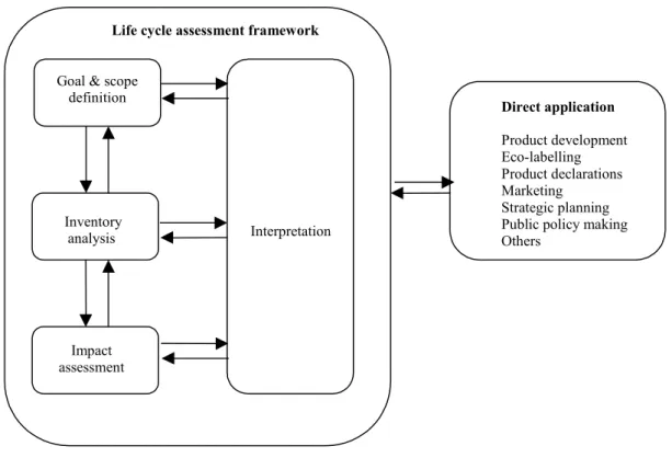
Figure 2.1 presents the ISO framework for LCA (ISO EN 14040 1997). An important notion of ISO EN 14040 is the iterative character of LCA. All phases may have to be passed through more than once due to new demands posed by a later phase. Though decisions and actions may follow the interpretation phase, these decisions and actions in themselves are outside the framework of LCA. However, possible “direct applications” are indicated in ISO EN 14040.
Figure 2.1: The phases of an LCA according to ISO EN 14040 (1997).
The goal definition clarifies the initial reasons, the intended application and the audience of the LCA. The main applications supported by LCA usually ask for a comparative assertion. That means, either comparison of different products that are functionally equivalent, or comparison of the processes within the life cycle of one product.
The scope definition specifies the object of the LCA and directs the specific methodology to be followed in the next phases. It also defines the basis on which the relevant products are compared. A particular product can provide different services and a given service can be provided by different products. The object studied in a LCA is therefore a product service
Life cycle assessment framework
Inventory analysis Impact assessment Interpretation Direct application Product development Eco-labelling Product declarations Marketing Strategic planning Public policy making Others
Goal & scope definition
rather than a product itself. The functional unit, a measure for the service performance of a product, ensures that the comparison is made on a common basis. The methodological
choices about boundaries and procedures for the other phases are according to ISO EN 14040 specified in scope definition.
Inventory analysis identifies and quantifies the resource extractions and consumptions, and
the releases to the environment relating to the processes that make up the life cycle of the examined product(s). These environmental inputs and outputs are expressed as quantities per functional unit (and do not contain a specification of the temporal and spatial characteristics of these).
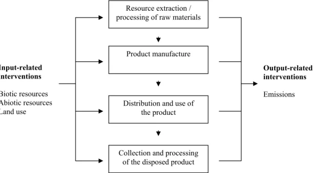
The life cycle of a product consists roughly of four stages. Figure 2.2 gives a schematic overview of the life cycle of an arbitrary product. However, each stage may consist of a number of processes which each uses one or more inputs from previous processes and gives outputs to one or more next processes. Consumption (and the preceding production) of energy, and transportation processes do take place in practically all stages.
Figure 2.2: Schematic overview of the life cycle of an arbitrary product and its inputs to, and outputs from the environment.
Each input to a process can be followed upstream to its origin (“cradle”) and each output to a process downstream to its final end (“grave”). The total of connected processes is called the product system, process tree or life cycle. It is easy to imagine that a product system can become rather complex as a product consists of more than one material or component. Even one material or component may represent a complex subsystem, however: A material like polyamide can be synthesised by many, very different technologies, and several producers can apply each technology.
Output-related interventions Emissions Input-related interventions Biotic resources Abiotic resources Land use Product manufacture
Distribution and use of the product
Collection and processing of the disposed product
Resource extraction / processing of raw materials
The system boundaries determine which processes will be included in the LCA. The definition of the product system and its boundaries takes, according to ISO EN 14040 and 14041, place in scope definition. Scope definition decides also for which environmental inputs and outputs data should be collected, and about the procedure to allocate these to processes with multiple outputs to next processes. The inventory phase therefore only consists of the actual data collection and data processing. Inventory analysis results in an inventory table where environmental inputs and outputs are listed and are summed-up per type of intervention. A sector-specific aggregation of the inputs and outputs can be performed in addition, indicating quantitatively in which stages of the life cycle the interventions occur or, the other way round, this information should not be lost during aggregation to the final inventory table.
Environmental inputs and outputs have the potential to bring about several kinds of impact on the environment (impact categories in LCA terms). Life cycle impact assessment estimates the potential contributions from these inputs and outputs to a number of impact categories and may choose to continue by weighting across impact categories in order to reduce the collection of impact categories into one measure.
As a first step, impact categories and category indicators should be selected together with the models to quantify the contribution to the selected impact categories and category indicators. Once these selections have been made, the environmental inputs and outputs are assigned to the impact categories selected in scope definition (classification). The contribution to an impact category from each input or output is then next modelled (characterisation). In very specific cases and only when meaningful, the modelling results for one impact category or subcategory may be aggregated with those of another one (grouping and weighting). The next section provides some more information about the impact assessment phase.
Life cycle interpretation is the phase in which the results of the inventory phase and the
impact assessment phase are combined in line with the defined goal and scope. Conclusions and recommendations to the decision-maker may be drawn, unless reviewing and revising of previous phases is needed. Both concluding/recommending and reviewing/revising should preferably be based on uncertainty and sensitivity analysis.
2.3 The impact assessment phase
According to ISO EN 14042 (2000), life cycle impact assessment consists of four mandatory elements and two optional elements:
• Selection of impact categories, category indicators and characterisation models (mandatory),
• Assignment of results from the inventory phase to the selected impact categories (classification; mandatory),
• Calculation of category indicator results with help of selected models (characterisation; mandatory),
• Calculating the magnitude of category indicator results relative to reference values(s) (normalisation; optional),
• Grouping or weighting (optional, weighting not allowed in comparative assertion disclosed to the public), and
• Data quality analysis (mandatory in comparative assertion).
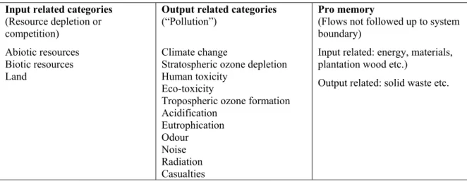
Udo de Haes (1996) provides a default list of impact categories in LCA (see Table 2.1). The list is not meant as a minimum and neither as a maximum list. The impact categories from this list that are relevant in this report are climate change, stratospheric ozone depletion, tropospheric ozone formation, acidification and eutrophication.
According to ISO EN 14042 (2000), a category indicator is identified as the quantifiable representation of an impact category, being the object of characterisation modelling. The category indicator can be defined at any level of the causality chain or chain of environmental mechanisms within an impact category that cause an environmental intervention to have an impact on the final endpoints. An example regarding climate change may illustrate this. The environmental mechanisms connecting an intervention (e.g. a CO2 emission) to the final
impact on its endpoints (e.g. damage to flora, fauna and human beings) may be:
Emission of CO2 → increased radiative forcing → climate change (i.e., average global
temperature rise, other climate changes) → rise of sea level → flooding of land → damage to ecosystems and human beings (e.g., expressed as years of human life lost). The category indicator for climate change is typically the increased radiative forcing and this radiative forcing is typically quantified with help of the Global Warming Potentials (GWP) as reported by the Intergovernmental Panel on Climate Change (Houghton 1996).
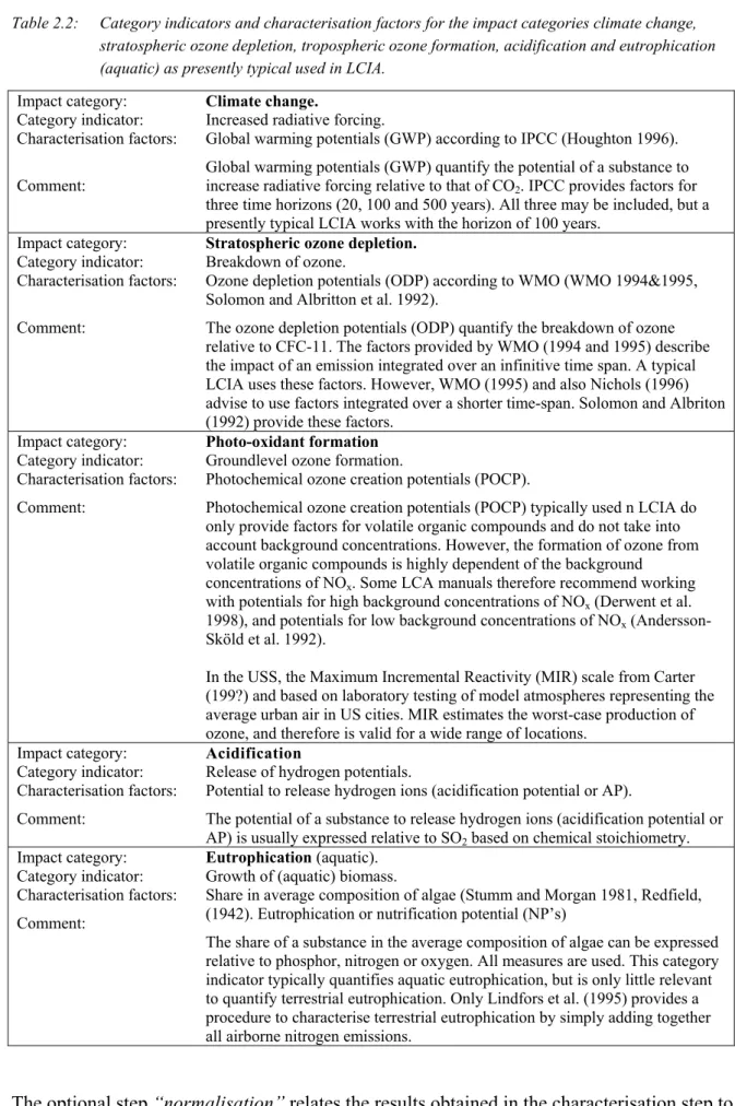
Table 2.2 lists the category indicators and models presently typically selected for the other impact categories being subject of this report. Presently typical characterisation in LCA uses equivalency or characterisation factors5.
Table 2.1: Default list of impact categories to be characterised in LCA (after Udo de Haes 1996)
Input related categories (Resource depletion or competition)
Abiotic resources Biotic resources Land
Output related categories (“Pollution”)
Climate change
Stratospheric ozone depletion Human toxicity
Eco-toxicity
Tropospheric ozone formation Acidification Eutrophication Odour Noise Radiation Casualties Pro memory
(Flows not followed up to system boundary)
Input related: energy, materials, plantation wood etc.)
Output related: solid waste etc.
Classification is the second mandatory element of the impact assessment phase and consists
of assigning data from inventory analysis to the relevant impact categories. One intervention may well be included in more than one impact category. An emission of NOx, for example,
contributes to acidification as well as to eutrophication.
Characterisation quantifies the contribution of an intervention to the relevant impact
categories. The category indicator - like the increased radiative forcing in climate change - is the quantifiable representation of an impact category. Characterisation factors - like the global warming potentials for climate change – are used to convert the environmental inputs and outputs assigned to a given impact category into their contribution to that impact
category at the level of the category indicator. The characterisation results in the
contributions to a number of impact categories, also indicates as the environmental profile of a product. Table 2.2 lists the presently typical characterisation factors related to the impact categories and category indicators being subject of this report.
5 Equivalency or characterisation factors represent models that establishing linear relations between emissions
and their impact on the environment at the level in the causality chain where the category indicator is defined. Such factors are simple in use, which does not necessarily mean they inaccurately characterise impact as these factors can be derived from underlying sophisticated models (i.e., they are meta-models of these sophisticated models).
Table 2.2: Category indicators and characterisation factors for the impact categories climate change, stratospheric ozone depletion, tropospheric ozone formation, acidification and eutrophication (aquatic) as presently typical used in LCIA.
Impact category: Category indicator: Characterisation factors: Comment:
Climate change.
Increased radiative forcing.
Global warming potentials (GWP) according to IPCC (Houghton 1996). Global warming potentials (GWP) quantify the potential of a substance to increase radiative forcing relative to that of CO2. IPCC provides factors for
three time horizons (20, 100 and 500 years). All three may be included, but a presently typical LCIA works with the horizon of 100 years.
Impact category: Category indicator: Characterisation factors:
Comment:
Stratospheric ozone depletion. Breakdown of ozone.
Ozone depletion potentials (ODP) according to WMO (WMO 1994&1995, Solomon and Albritton et al. 1992).
The ozone depletion potentials (ODP) quantify the breakdown of ozone relative to CFC-11. The factors provided by WMO (1994 and 1995) describe the impact of an emission integrated over an infinitive time span. A typical LCIA uses these factors. However, WMO (1995) and also Nichols (1996) advise to use factors integrated over a shorter time-span. Solomon and Albriton (1992) provide these factors.
Impact category: Category indicator: Characterisation factors: Comment:
Photo-oxidant formation Groundlevel ozone formation.
Photochemical ozone creation potentials (POCP).
Photochemical ozone creation potentials (POCP) typically used n LCIA do only provide factors for volatile organic compounds and do not take into account background concentrations. However, the formation of ozone from volatile organic compounds is highly dependent of the background
concentrations of NOx. Some LCA manuals therefore recommend working
with potentials for high background concentrations of NOx (Derwent et al.
1998), and potentials for low background concentrations of NOx
(Andersson-Sköld et al. 1992).
In the USS, the Maximum Incremental Reactivity (MIR) scale from Carter (199?) and based on laboratory testing of model atmospheres representing the average urban air in US cities. MIR estimates the worst-case production of ozone, and therefore is valid for a wide range of locations.
Impact category: Category indicator: Characterisation factors: Comment:
Acidification
Release of hydrogen potentials.
Potential to release hydrogen ions (acidification potential or AP).
The potential of a substance to release hydrogen ions (acidification potential or AP) is usually expressed relative to SO2 based on chemical stoichiometry.
Impact category: Category indicator: Characterisation factors: Comment:
Eutrophication (aquatic). Growth of (aquatic) biomass.
Share in average composition of algae (Stumm and Morgan 1981, Redfield, (1942). Eutrophication or nutrification potential (NP’s)
The share of a substance in the average composition of algae can be expressed relative to phosphor, nitrogen or oxygen. All measures are used. This category indicator typically quantifies aquatic eutrophication, but is only little relevant to quantify terrestrial eutrophication. Only Lindfors et al. (1995) provides a procedure to characterise terrestrial eutrophication by simply adding together all airborne nitrogen emissions.
The optional step “normalisation” relates the results obtained in the characterisation step to the total indicator result of a country, region or the world. The ratios thus obtained for the
different categories provide an indication for the relative importance of the categories in the context of a specific LCA study, if the same reference area is taken for all categories. This constitutes, of course, a kind of weighting but it does not involve the societal values necessary in weighting in the more narrow sense used in ISO 14042.
The optional step “weighting” tries to establish an hierarchy of the categories, either within the framework of a specific LCA study, or in general. Inevitably, weighting requires societal values and, thus, cannot be done with the methodology of the (exact) sciences. Weighting, although excluded by ISO 14042 for use in comparative assertions to be disseminated in the public, is often regarded necessary in comparative LCAs, since the results of the impact assessment are in most cases not unambiguous, showing bad ratings in some categories and good ones in others.
2.4 Focus of the work
According to ISO EN 14042 (2000), life cycle impact assessment consists of four mandatory elements (selection, classification, characterisation and data quality analysis) and two
optional elements (normalisation and grouping & weighting). The elements of normalisation, and grouping & weighting can thus follow upon characterisation but are not mandatory. It is left optional whether or not to perform these elements, though weighting is not allowed in comparative assertion disclosed to the public.
Normalisation and grouping and weighting have been subject of intensive debate in the ISO-process because of the subjectivity involved in performing these elements. An important group of LCA practitioners is reluctant towards weighting in particular, but even as many practitioners consider weighting an unavoidable element since no explicit weighting leads to implicit weighting. Weighting and/or aggregating the different category indicators is usually necessary to compare product systems or evaluate improvement options, since one alternative hardly ever scores better on all category indicators than the other alternative.
Some practitioners attempt to minimise the subjectivity from weighting (i.e. to partly avoid weighting) by choosing their category indicators further along the causality chain, close to or at the endpoint point and expressing the impact on the endpoint in the same unit (facilitating aggregation of indicators without weighting). This reduces the number of category indicators to be weighted and aggregated since the number of endpoints is limited and several impact categories therefore share their indicator. However, an important question is whether the state-of-the art does yet allow to model up to the endpoint. This is subject of the next chapter. The focus of SETAC-Europe/STG-GARLIC is on best available practice(s) in
characterisation. Best available practice in characterisation is not necessarily best available practice in weighting. These are two different optimisations that at the present-state-of-the-art
may prompt to acceptance of “less” than best available practice in one of the two elements. That is, prioritising easiness of weighting by choosing category indicators with the same unit (i.e. avoiding weighting) may require “less” than best available practice in characterisation (and the other way around).
The choice to optimise either towards characterisation or to weighting by modelling further along the causality chain depends on the application and context of the given LCA, but there is thus a tension between best available practice(s) in characterisation and best available practice(s) in weighting in LCA. The next chapter touches upon this tension, but does not further address the issue of weighting since another Scientific Task Group deals with this element and also with grouping and normalisation.
3
Sophistication of category indicators
3.1 Introduction
The impact assessment phase in LCA is relatively young and emerged from the wish to simplify the large amount of data from inventory analysis by aggregation into a manageable number of impact indicators. This wish has in the course of time been extended with the wish to increase the environmental relevance of the impact assessment phase in LCA.
Discussions about the environmental relevance of impact assessment in LCA has long been dominated by two closely connected issues: evaluation of threshold exceedance (Section 3.2) and spatial (and temporal) differentiation (Section 3.3) in characterisation of impact. These issues and thus this chapter are particularly relevant for the non-global impact categories. The discussion about whether or not to perform evaluation of threshold exceedance has last few years shifted towards the question whether characterisation should go beyond threshold evaluation (risk analysis) and focus on quantification of subsequent damage. In other words, at which level within the causality chain (see also Section 2.3) should category indicators preferably be defined in LCA: somewhere in between emissions and endpoint (a so-called mid-point indicator), or at the endpoint (so-called endpoint indicator).
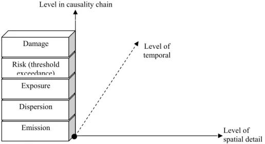
Figure 3.1: Levels of possible spatial and temporal sophistication in LCA and levels at which the category indicator can be defined.
The level at which category indicators are chosen is one form of sophistication. Another form of sophistication is the extent to which spatial and temporal resolution is taken account in the characterisation modelling up to the chosen level in the causality chain. The chosen level of
Emission Dispersion Exposure Risk (threshold exceedance) Damage
•
Level of spatial detail Level of temporal Level in causality chainspatial and temporal differentiation can thus be seen as a sophistication perpendicular on the chosen level in the causality chain at with the category indicator is defined (see Figure 3.1). This also presages the close relation between chosen level of spatial and temporal resolution on the one hand and the level in the causality chain at which the category indicator is defined on the other hand as will be further clarified in this chapter.
3.2 Position of category indicators
3.2.1 The threshold issue
The first generation characterisation methods took their basis in equivalency assessment with help of characterisation factors that were derived from intrinsic substance characteristics like the potential to release hydrogen ions (for acidification assessment), toxic effect-levels (for toxicity assessment)6 or the ability to radiative forcing (for climate change). Modelling of exposure and assessment of threshold exceedance (i.e. PEC/PNEC ≥ 1)7 were not performed
since the available data did not allow such evaluation.
Threshold information, usually in the form of a no-effect-level, was in the first generation characterisation models thus used only in toxicity assessment to express the emission of a given substance as a dilution volume of the receiving environment. The basis of equivalency was taken in the toxicity potential of each substance by setting to one for the impact from an emission quantity equal to the no-effect-level8, and the impact from any deviating quantity as the ratio of the emission quantity divided by the no-effect-level.
6 No-effect-concentrations are based on experiments on test-species under laboratory conditions and therefore
say something about the intrinsic substance characteristic to cause toxic effect (rather than something about the sensitivity of a species in real-life for this toxic substance).
7 “PEC” stands for Predicted Environmental Concentration, and “PNEC” for Predicted No Effect Concentration. 8 The underlying assumption is that the toxicity impact from a quantity at the no-effect-level of one substance
has the same importance as the toxicity impact from a quantity at the no-effect-level of another substance. To put it more clearly: If the quantities of both substances are at their no-effect-level, the impacts from a neuro-toxic substance and a skin irritating substance are regarded as equally important. The adding together of very different effect types is one of the more serious problems in LCA, but is not further addressed in this document.
Present toxicity factors now also cover exposure modelling that quantifies the change in exposure from an emission (rather than the total exposure resulting from the emission). The aggregation of the calculated exposure increases from different substances is still often based on no-effect-levels. Toxicity impact is now defined as the change in predicted environmental concentration (i.e., change in exposure) divided by the – predicted – no-effect-concentration (∆PEC/PNEC).
Evaluation of threshold exceedance is still not covered by the present generation of toxicity factors, however, and neither feasible in the context of characterisation of toxicity. Such evaluation needs information about operative background exposures on top of which an exposure increase takes place. There are simply too many potential toxic substances that make such information yet hard to achieve within the present state-of-the-art science in toxicity assessment.
Though evaluation of threshold exceedance was initially not performed due to lack of data, it has meanwhile turned for some practitioners into a principle in itself that is justified by the reasoning that “less pollution is better”. An important other group of practitioners has always been advocating an “only above threshold” approach on the other hand. An impact
assessment following an “only above threshold” approach accounts only for those emissions leading to exposure levels above threshold.
The discussion whether to perform evaluation of threshold exceedance in LCA is topical for already quite some years now but has mainly taken place in relation to toxicity assessment. However, recent publications of Potting et al. (1998), Pleijel et al. (not published), Lindfors et al. (1998), Huijbregts et al. (2000), Hauschild and Potting (2003), Potting and Hauschild (2003) and Krewitt et al. (2001) show evaluation of threshold exceedance to be quite well possible for the impact categories photo-oxidant formation, acidification and terrestrial eutrophication with help of characterisation factors simple to use in LCA. These
characterisation factors are derived from sophisticated underlying models and can thus be seen as meta-models summarising the sophisticated modelling in a linear relation between emissions and their impact at the level in the causality chain where the indicator is defined. These publications actually also show that more approaches are possible than “less pollution is better” and “only above threshold” only. Few of them are described in the following section.
3.2.2 Threshold based category indicators
In a “less pollution is better” approach, all emissions are considered to be relevant on the basis of their intrinsic harmful properties. The assumption initially underlying the “less pollution is better” approach is that all emissions give rise to exposure increases at sites that have a similar sensitivity to the given substance. Recent work of Huijbregts et al. (2000)
takes a somewhat more sophisticated approach. Huijbregts et al. used the RAINS-model9 to calculate characterisation factors for acidification and terrestrial eutrophication that do allow ecosystems to have different a priori tolerances for exposure increase (each ecosystem has its own critical load)10, but does not take into account differences in background exposure. His definition of the category indicator is similar as to the one that – by necessity – is typically used in toxicity assessment (see also Section 3.2.1). Impact on the individual ecosystem is defined by Huijbregts et al. as the predicted exposure increase divided by the critical load of the given ecosystem11,12. This results in the impact from an exposure increase on an
ecosystem exposed just below its critical load (and thus about to be in danger) regarded equally important as an ecosystem facing the same exposure increase but already exposed far above its critical load (and thus difficult to rescue). Similarly, the impact from exposure increases on these ecosystems are regarded equally important as an ecosystem facing the same exposure increase but still exposed far below its critical load (and thus hardly in danger). Whether ecosystems are thus exposed far below or at or far above their critical loads, they are all characterised as equally vulnerable by Huijbregts et al.. An ecosystem with a high critical load is on the other hand taken as more vulnerable than an ecosystem facing the same exposure increase but having a low critical load.
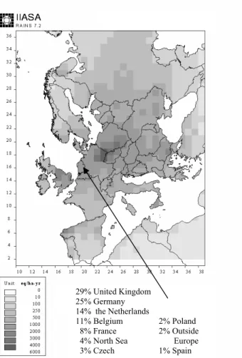
9 The RAINS model provided the model calculations being at the basis of the several protocols under the
CLRTAP. It is an 'easy-to-use' computer tool that combines spatial resolved information on regional emission levels with information on long-range atmospheric transport to estimate patterns of deposition and concentration for comparison with critical loads and thresholds for acidification, terrestrial eutrophication and tropospheric ozone formation in Europe. See Chapter 5 for more information.
10
So are the Scottish moors very intolerant towards acidifying loading in contrast with the ecosystems on the rather insensitive lime soils in South Europe.
11 As a matter of fact, the a priori tolerance of ecosystems for acidifying loading is described by critical load
functions (rather than by one unique value per substance). The critical load function gives all combinations of
sulphur and nitrogen deposition above which an ecosystem is at risk to be damaged (see Posch et al. 1995). For the sake of clarity, the term “critical load” is used in this paper in stead of the correct term “critical load function”.
12 The non-existence of a unique critical load for given acidifying substances (see previous footnote)
complicates the approach of Huijbregts et al. (since the denominator is not a fixed value, but is depending on the loading of other acidifying substances). Huijbregts et al. solves this by using the maximum critical sulphur and nitrogen load. Another possibility would have been to work with the critical sulphur and nitrogen loads as uniquely defined by the exceedance function (i.e., the point that provides the “shortest” distance to exceedance of the critical load function; see Posch et al. 1999). Such approach would be in accordance with the work done under the UNECE convention on long range transboundary air pollution (see also Chapter 3), and also facilitates to address exceedance of the critical loads in a consistent and comparable way (see also Section 5.5). The characterisation factors of Lindfors et al. (1998) and Potting et al. (1998) are both based on critical load
An “only above threshold” approach considers only those emissions relevant that result in exposure increases at sites where critical loads are already exceeded. Impact on the individual ecosystem is valued to be one for any exposure increase on top of an exposure already being above the critical load of the given ecosystem. An ecosystem exposed far above its critical load (and thus difficult to rescue) is considered to be equally vulnerable as an ecosystem exposed just above its critical loads (and thus relatively easy to rescue). The impact from an exposure increase is on the other hand valued as zero for all ecosystems being exposed below their critical loads. This applies to ecosystems exposed far below their critical loads (and thus hardly in danger) as well as to ecosystems exposed just below their critical loads and thus in danger to become above their critical load by a small exposure increase.13 “Only above threshold” approaches nevertheless take into account the a priori tolerances and differences in background exposures of ecosystems in order to evaluate whether the critical loads of the given ecosystems are already exceeded. Pleijel et al. proposed, and Lindfors et al. (1998) subsequently established “only above threshold” factors14 for acidification and terrestrial
eutrophication with help of models parental to the RAINS-model.
Potting et al. (1998) introduced an approach alternative to the two previous ones and that could be called “only around threshold”. This approach gives priority to ecosystems exposed around their critical load rather than to ecosystems exposed far below (and thus hardly in danger) or ecosystems exposed far above (and thus difficult to rescue). The work of Potting et al. should be evaluated against the fact that the emission of one source (i.e. one process) contributes to many ecosystems (far more than hundred thousand). Each of these ecosystems may differ in their operative background exposures, but they can also differ in a priori tolerance for exposure. Potting et al. based their characterisation factors on the slope of the curvilinear (sigmoid) dose-effect curve that is defined by the critical loads of all ecosystems to which one source contributes. The slope of this dose-effect curve is established with help of the RAINS-model in the working point that is thus determined by the operative
background exposure. The resulting characterisation factors of Potting et al. quantify the area of ecosystems that becomes exposed above their critical loads as a result of the exposure increase from our functional unit. The “only around threshold” characterisation factors express the sensitivity of a “population” of exposed ecosystems for the changes in their background loading evoked by a given source15. The factors thus account for both differences
in ecosystem a priori tolerance for loading and differences in background load. In this way,
13 As is clear from the before discussion, “only above threshold” factors do not characterise emissions on the
basis of the change in impact that they invoke, but on the basis of the existing impact from the operative background loads. This assumes that the considered emissions do not evoke any change in that impact. This makes “only above threshold” characterisation to a so-called average approach.
14 The factors of Pleijel et al. and Lindfors et al. are as a matter of fact no characterisation factors but modifiers
to be used in combination with the hydrogen release potentials for acidification and the biomass production potentials for eutrophication (see Table 3.2 in Chapter 3). The modifier expresses what share of the emission from a given region deposits on ecosystems with background loads above their critical loads.
15 To be useful in LCA, characterisation factors should not be too sensitive for changes in the background
exposure of receptors (see also Section 5). Potting et al. (1998a) showed that the “only around threshold”
ecosystems are prioritised that are exposed close to their critical load (and thus about to be in danger or just above the critical load and therefore relatively easy to rescue). Hauschild and (2003) and Potting and Hauschild (2003) established “only around threshold” characterisation factors for acidification, terrestrial eutrophication and groundlevel ozone formation.
A critical load can only tell whether there is a risk on ecosystem damage, but not whether this risk actually results in damage and how large this damage is. One nevertheless expects the damage to become (asymptotically) larger with increasing exceedance of a critical load. More sophisticated would therefore be to follow a damage approach. Goedkoop and Spriensma (2000) go in the direction of such approach by quantifying, in the case of acidification and terrestrial eutrophication, the fraction of vascular plant species potentially disappeared as a result of a change in deposition. An advantage of this approach, and also the initial reason to develop it, is that acidification and terrestrial eutrophication can be aggregated since they are expressed in the same unit. Similarly to Potting et al., the damage factors from Goedkoop and Spriensma are calculated as the slope of the dose-damage curve established in the working point that is determined by the operative background exposure. The damage factors are calculated with help of the so-called Nature Planner. This model is comparable with the RAINS-model, but the model domain of the Nature Planner is limited to the Dutch territory, which does not allow spatial resolved impact factors16.
3.2.3 Midpoint – endpoint modelling
The previous section discussed a number of category indicators using threshold information (or damage information in the last one). The above list of indicators is not exhaustive. More definitions are possible, like for instance so-called fate-factors from Norris in Bare et al. (2003) that quantify which share of an emission deposits on land (regardless whether on ecosystem area or otherwise). The discussed selection of indicators is summarised in Table 3.1.
An interesting feature about the category indicators in Table 3.1 is that they are defined increasingly further in the causality chain. Closer to the endpoint thus. This may in practice lead to a change in relative importance between substances assigned to an impact category. For example, the importance of nitrogen relative to sulphur decreases for category indicators defined further along the causality chain compared to an indicator defined at the begin-point (like the hydrogen release potential). This is due to the fact that deposition of nitrogen will often be assimilated by ecosystems and then does not contribute to acidification, or deposits on ecosystems not sensitive to the emission. Sort-like “corrections” in the characterisation factors are gained for other impact categories if their category indicator is defined further along the causality chain.
Defining category indicators further along the causality chain thus adds to the environmental relevance of the quantification of the selected impact categories (provided that the underlying modelling is sound). However, the additional environmental relevance remains small as long as the modelling further along the causality chain is not combined with spatial (and temporal) differentiation. This is subject of the next sections.
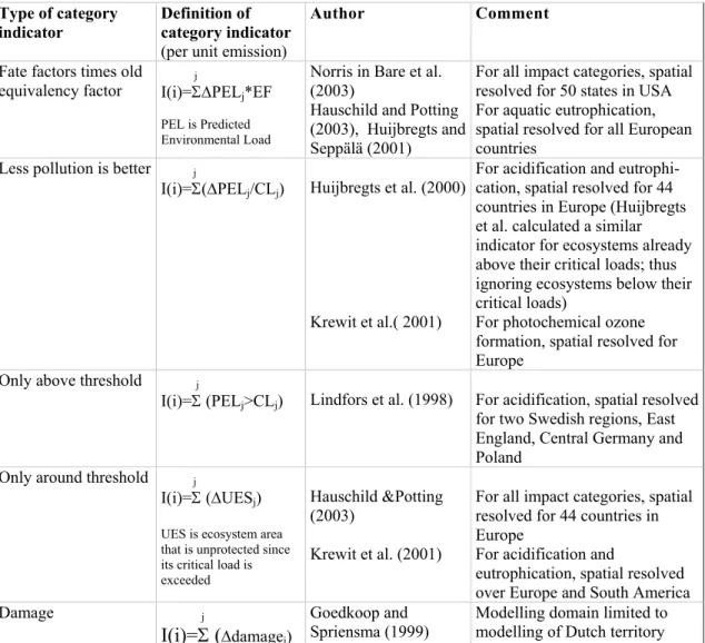
Table 3.1: A selection of category indicators that are available for characterisation modelling in LCA.
Type of category
indicator Definition of category indicator (per unit emission)
Author Comment Fate factors times old
equivalency factor I(i)=Σ∆PELj j*EF
PEL is Predicted Environmental Load
Norris in Bare et al. (2003)
Hauschild and Potting (2003), Huijbregts and Seppälä (2001)
For all impact categories, spatial resolved for 50 states in USA For aquatic eutrophication, spatial resolved for all European countries
Less pollution is better j
I(i)=Σ(∆PELj/CLj) Huijbregts et al. (2000)
Krewit et al.( 2001)
For acidification and eutrophi-cation, spatial resolved for 44 countries in Europe (Huijbregts et al. calculated a similar indicator for ecosystems already above their critical loads; thus ignoring ecosystems below their critical loads)
For photochemical ozone formation, spatial resolved for Europe
Only above threshold j
I(i)=Σ (PELj>CLj) Lindfors et al. (1998) For acidification, spatial resolved
for two Swedish regions, East England, Central Germany and Poland
Only around threshold j
I(i)=Σ (∆UESj)
UES is ecosystem area that is unprotected since its critical load is exceeded
Hauschild &Potting (2003)
Krewit et al. (2001)
For all impact categories, spatial resolved for 44 countries in Europe
For acidification and
eutrophication, spatial resolved over Europe and South America Damage j
I(i)=Σ (∆damagej)
Goedkoop and
Spriensma (1999) Modelling domain limited to modelling of Dutch territory
16 Acidifying and eutrophying substances typically travel over distances of several hundreds to thousand
3.3 Resolution aspects
3.3.1 Spatial differentiation
The long distance transport of emissions means that one has to look over several hundreds to thousands kilometres to catch most of the impact from a source. The large impact area of an emission makes the precise location of a source of less importance because the dispersion patterns and impact area of neighbouring sources overlap (i.e. show largely the same gradients). Dispersion patterns and impact area will only start to deviate considerably when sources are located at larger distances from each other. This makes it possible to establish so-called site-dependent factors that characterise impact somewhere between site-generic and site-specific and that with reasonable good accuracy estimate the impact from a source located in a given region on its receiving environment:
Site-generic Site-dependent characterisation Site-specific
characterisation characterisation
It is important that spatial resolved characterisation in LCA does not put unfeasible demands for additional data on inventory analysis (see also Section 3.3.3). Therefore, the resolution of site-dependent characterisation factors should be kept as low as possible. Hence that spatial resolution here refers to the size of the distinguished source regions for which site-dependent factors are established (and not to the spatial resolution of the modelling underlying those factors; this resolution can be and is typical fairly high).
Site-dependent factors for acidification, terrestrial eutrophication and tropospheric ozone formation have been established for North America and Europe (an overview is given in Table 3.1). These factors express the impact from an emission in a given region over its full impact area.
Site-dependent characterisation factors for each state in North America are established by Norris in Bare et al. (2003). These factors represent so-called fate factors that quantify the share of emissions leading to concentration or exposure increases on land surface (he does not quantify which receptors are exposed and whether they are sensitive to this).
Several sets of spatial resolved characterisation factors are available for the 44 countries forming together Europe. Most of these sets are based on different definitions of the category indicator (see Section 3.2.2). The factors of Hauschild and Potting (2003) and Guinée et al (in preparation) are derived with help of the RAINS model and the ones of Lindfors et al. (1998) with help models parental to RAINS. The factors from Krewit at al. (2001) are calculated with the EcoSense, a model comparable to RAINS. The acidification and eutrophication factors or Hauschild and Potting (2003) and Krewit et al. (2001) are based on the same definition of the category indicator.
Potting and Hauschild (2003) made a comparison between the fate-factors or the “less
pollution is better” factors of Huijbregts et al. (2000), and the “only around threshold” factors of Hauschild and Potting (2003). All sets of spatial resolved acidification and eutrophication factors were calculated with help of RAINS and can be regarded as based on a category indicator defined increasingly closer to the midpoint. A number of interesting conclusions can be draw from this comparison:
• The range of values is relative small for the spatial resolved fate-factors (less than a factor 10 between lowest and highest value) but becomes increasingly larger as the category indicator is defined further along the causality chain (factor hundred for “less pollution is better” factors and a factor thousand for “only around threshold” factors between lowest and highest value). Spatial differentiation thus becomes more important if the category indicator is chosen closes to the endpoint.
• A site-generic characterisation factor for the “less pollution is better” and “only around threshold” factors, as mean value from the set of spatial resolved factors, is strongly influenced by the regions selected (e.g., EU15, EU15+Norway+Switzerland, East Europe or all 44 European countries). The standard deviation for each set is about 100% of the mean value. Site-generic characterisation by refraining from spatial differentiation thus results in a considerable uncertainty in the category indicator.
• There is a considerable variation in mean value for selections of large neighbouring regions (like East Europe and EU15+Norway+Switzerland). Site-dependent factors for small neighbouring regions (like Belgium and the Netherlands) are on the other hand quite similar. This means that characterisation factors can be resolved over rather large regions, but these regions should not be too large. About 500*500km resolution seems adequate. Such resolution will often comply with the size of countries or larger
administrative regions within large countries.
3.3.2 Temporal differentiation
The small or marginal contribution from a single source to exposure of its receptors means that the time behaviour of the emission from that source (i.e. whether it is a flux or pulse) becomes less important. The temporal variation of the contribution from a single source will usually namely to a large extent be cancelled out against the high background exposure from all sources together. Exposure of receptors thus show a relative invariability in time for the contribution of single sources (this does not imply the opposite reasoning, that the temporal variations in the total exposure of receptors is unimportant).
If the exposure of receptors shows a relative invariability in time for the contribution of a single but full source, the same of course inherently holds true for the emission per functional
unit. The temporal variation of emissions is thus of minor importance in characterisation modelling in LCA. This is an important observation since the lack of information about the temporal variations in emissions has long been an issue of intensive debate in LCA. The calendar time to which the different processes in a product system relate is a more important issue when it comes to impact assessment in LCA. The calendar time of a process determines the (estimated) total economic activity with all its emissions being responsible for the total environmental load causing an impact to which background that process adds. The background situation can be rather different between calendar times (and thus between different processes in an LCA as discussed below). This could result in rather different
characterisation factors related to these different calendar times (since “only above threshold” and “only around threshold” factors do account for background exposures; see Section 3.2.2). The photochemical ozone creation potential from an emission of a volatile organic compound may be different in 1990 and 2010 due to considerable differences in the background
concentration levels of nitrogen oxides posed by the total economy in those years.
A product can easily cover a time frame of several decades depending on time-of-use of the product and the time needed for each subsequent process in the product system. For example, a linoleum floor covering will on average first be discarded 15 years after is has been bought (Potting and Blok 1995). The factors used to characterise the impact from a given process should relate to the calendar time in which that process takes place (a time-dependent characterisation factor thus).
As a matter of fact, also processes themselves can cover a time frame of several years to decades. A specific type of linoleum will be produced over a certain time interval before the type is taken from the market. This determines the time or calendar interval over which that type is marketed, used and disposed. Basically, the used characterisation factor should thus not relate to the calendar time, but to the calendar interval in which a given process takes place.
Similar to spatial differentiation, the level of temporal differentiation can be placed on a continuum stretched up by the two extremes time-specific and time-generic characterisation. Time-dependent characterisation has thus a level of detail somewhere between those
extremes:
Time-generic Time-dependent characterisation Time-specific
characterisation characterisation
Time-dependency has been explored by Potting and Hauschild (2003) and also by Krewit et al. (2001) by establishing “only around threshold” factors for 1990 and 2010. Trends in the site-dependent factors remain roughly the same across countries, though 2010 factors are
considerable lower than 1990 factors. This is an obvious result since emissions projections between 1990 and 2010 are considerably different. Without going into details, however, trend analysis shows emission projections to be relatively stable over a couple of years (Jol and Kielland 1997). This suggests a time dependent assessment based on time-intervals of several years to be adequate for LCA. Time-dependency seems to be one of the coming issues in LCA.
3.3.3 Data availability
Application of site-dependent characterisation factors requires rough information about the geographical region where a process and its emission takes place. Similarly, a time dependent characterisation requires information about the years over which an emission is expected to take place. A major objection against site-dependent (and time-dependent) characterisation in LCA is that the demand for this data should cause unfeasible complications for inventory analysis. This has also been subject of intensive discussion between the authors of this report. Some main lines are drawn here.
Before outlining the discussion, it may be interesting to observe that unfeasible complications for inventory analysis of additional data demand are never put so prominently forwards as in relation to site-dependent characterisation in LCA. This is somewhat surprising since there are a number of recent extensions to LCA methodology that never received the same
resistance, though they certainly require considerable additional data and they do complicate inventory analysis. Examples are expansion of product systems to avoid allocation as also recommended by ISO EN 14041, and the adoption of several new impact categories asking for new inventory items to be collected.
Let’s return to the issue and further focus on site-dependent characterisation (the discussion will be roughly the same for time-dependent characterisation, but no concrete methodology is yet available here). An indications of the region where a process and its emission takes place is usually readily available from goal & scoping and inventory analysis since this information is necessary to quantify transport within a product system. It also complies with meanwhile common sense between LCA practitioners that inventory analysis has to be more time specific and site-specific in order to improve the quality of inventory data (these
specifications are now also demanded by the SPOLD and SPINE data formats and several LCA databases).
It is important to stress that site-dependent characterisation does not ask for exact information about the location of a process. It is sufficient for site-dependent characterisation, as
discussed in Section 3.3.1, to identify the larger region where a process is located (countries or larger administrative regions within large countries; regions of roughly 500*500km).