Carbon capture by means of oxy-combustion in a gas turbine power plant, an assessment of the Allam cycle

(1)

cycle.

turbine power plant, an assessment of the Allam

Carbon capture by means of oxy-combustion in a gas

Academic year 2019-2020

Master of Science in Electromechanical Engineering

Master's dissertation submitted in order to obtain the academic degree of

Supervisors: Prof. Tom Verstraete, Dr. Samuel Saysset (Engie)

Student number: 01306228

(2)

(3)

cycle.

turbine power plant, an assessment of the Allam

Carbon capture by means of oxy-combustion in a gas

Academic year 2019-2020

Master of Science in Electromechanical Engineering

Master's dissertation submitted in order to obtain the academic degree of

Supervisors: Prof. Tom Verstraete, Dr. Samuel Saysset (Engie)

Student number: 01306228

(4)

Acknowledgements

I am grateful to have been able to complete this masters dissertation as a final assignment for obtaining of my mechanical engineering degree at the university of Ghent, where I have received a broad, qualitative and interesting education.

I would like to thank my supervisors: Tom Verstraete for his technical guidance and critical reflections on this work as well as his patience and motivational support, without which this project could not have been completed; Samuel Saysset for the enthusiasm with which he helped me navigate through the early stages of exploring a broad field of research, and technical assistance with modelling and simulations; my father and brother, Karel and Brecht Gyselinck, and my friend, Bob Van Leeuwen, who also provided useful feedback and suggestions in relation to this manuscript and showed a great interest and willingness to discuss the topic. They all have been a welcome support during this work. Most of all, I would like to thank my family and friends for being there and creating many happy moments together. This inspired me in my work and will continue to inspire me throughout life – AD 2020.

(5)

II

Abstract

Thesis: Carbon capture by means of oxy-combustion in a gas turbine power plant, an assessment of the Allam cycle. Student: Toon Gyselinck

Degree: Master of science in electromechanical engineering: mechanical energy engineering University: University of Ghent – UGent

Department: Faculty of engineering and architecture Supervisor: Prof. Tom Verstraete, Dr. Samuel Saysset Date: August 2020

Keywords: the Allam cycle, thermodynamic cycle analysis, oxy-combustion carbon capture, supercritical CO2

This thesis aims at becoming a useful addition to all the work concerning decarbonization of society and more specifically the power sector. Since a large share of electricity is generated by fossil fuels, the complete abatement of this energy resource seems unlikely in the short-term. A new concept for a power cycle is discussed and analysed: the Allam cycle. This cycle employs oxy-combustion to capture carbon dioxide generated by combustion of natural gas.

This study contains two parts. The first part sketches the context and background of the thesis’ subject, it is based on a literature review and online research: the first chapter shows graphs and figures concerning global energy requirements and CO2 emissions; the second chapter discusses the important aspects regarding carbon capture, usage and storage; the third

chapter discusses oxy-combustion and presents a comparison of several oxy-combustion power cycles that hold the greatest potential in terms of efficiency and cost; in the fourth chapter the Allam cycle is discussed from the perspective of the field of supercritical CO2 power cycles.

The second part focuses on the thermodynamic and technical aspects of the Allam cycle, it is both based on a literature review and original results, obtained by simulation of the cycle in Aspen Hysys. The literature provides modelling assumptions, a reference to which performance results can be compared, as well as describing some technical considerations regarding key equipment. This is discussed in chapter five. In the last and sixth chapter the results are presented and discussed. The simulations in Hysys are performed in a number of categories to assess the effect of various boundary conditions on the cycles’ operation, with the intent of identifying the operating state that gives the maximum cycle efficiency, which is found to be 54.44%.

It is concluded that the Allam cycle has a strong thermodynamic performance and is economically competitive with (even superior to, in some aspects) current power plant technologies The main advantages are: near-zero carbon emissions, low cost of CO2 avoidance, high plant efficiency, simple cycle configuration, a small plant footprint and competitive cost. There

are some uncertainties as well, because there is no operational experience with this cycle, operating at very high pressures, the combustor, turbine and recuperator must be designed and manufactured differently from existing equipment and may profit greatly from testing and advances in material development. Many research is being done and there are plans for building a commercial plant, so in the coming years the power of this plant will surely be proven.

(6)

Carbon capture by means of oxy-combustion in a gas

turbine power plant, an assessment of the Allam cycle.

Toon Gyselinck

Supervisors: Tom Verstraete, Samuel Saysset

Abstract In this study the Allam cycle is investigated. This,

rather novel, concept for generating electricity from fossil fuels while capturing the associated carbon dioxide employs two characteristic principles: oxy-combustion and a supercritical CO2 working fluid. The cycle was simulated in a process engineering program, Aspen Hysys, and several sensitivity analyses were performed. After recognizing the effects of combustion temperature (for example) and the importance of the recuperative heat exchanger, the operating states were optimized as to achieve maximum net cycle efficiency, resulting in a value of 54.44% (based on the LHV of the fuel – i.e. natural gas), while capturing 90% of the generated CO2.

Keywords Allam cycle, oxy-combustion, supercritical CO2,

cycle analysis, thermodynamic optimization

I. INTRODUCTION

In 2017, 406.7 EJ of energy was consumed, globally, from which 92.6 EJ under the form of electricity [1]. The majority of the electricity (64.5%) was generated by burning fossil fuels – in the first place coal and secondly natural gas. The power sector is responsible for the emissions of 13.6 Gt CO2, of which

12.9 Gt due to the use of coal and gas in thermal power plants [2]. As citizens and governments are waking up to the dangers of unrestrained global warming, many strategies for limiting greenhouse gas emissions have been proposed. One of these strategies is carbon capture, usage & storage (CCUS). To stay below 1.5 °C temperature rise, the IPCC models up to 1,200 Gt of CO2 being stored by 2100. [3]

There are several methods of capturing carbon from a thermal power plant, these are i) post-combustion capture: CO2 is

removed from the flue gas at the end of the power cycle, usually through absorption by a liquid sorbent, such as monoethanolamine (MEA); ii) pre-combustion capture: CO2 is

captured prior to fuel combustion, the hydrocarbon fuel is gasified and shifted to a syngas which is burned, CO2 is usually

removed during the gasification process by adsorption on a sorbent – such as activated carbon - which is desorbed from the CO2 in another column and then recirculated to the stripper

column; iii) oxy-combustion capture: the combustion of the fuel is done with pure oxygen instead of air, such that the flue gas contains only water vapor (H2O) and CO2, the CO2 can then

easily be separated from the mixture by water condensation; iv) chemical looping combustion (CLC): heat is released by a chemical reaction of the fuel with a metal-oxide, which serves as an oxygen carrier and circulates between two reactors: the fuel reactor and the air reactor - in the first reactor oxygen from the air binds to the metal-oxide which is subsequently sent to the fuel reactor, where the oxygen is released from the carrier

to react with the fuel, upon which the metal-oxide is circulated back to the air-reactor.

In this study a power cycle, called the Allam cycle, was investigated, which uses oxy-combustion to capture CO2. The

cycle shows potential for becoming a competitive (economically and thermodynamically) thermal power cycle compared to current coal- and gas-fired power plants.

II. INNOVATIVE THERMAL POWER CYCLES

The Allam cycle can be studied from both fields of research, oxy-combustion and supercritical CO2 cycles, which provides a broader perspective on its characteristics.

A. Main oxy-combustion power cycles

The oxy-combustion cycle promises a simple method for carbon capture. Several cycles have been developed since as early as 1985, when Herbert Jericha proposed the Graz cycle. The most notable are the semi-closed oxy-combustion combined cycle (SCOC-CC), the Allam cycle, the Graz cycle (variations are the S-Graz and Modified S-Graz cycle) and the CES cycle (developed by clean energy systems – variations include the revised and the supercritical CES cycle). These cycles have been developed both for combustion of natural gas and coal. The current study focusses on the natural gas-fired application of the power cycles, as it is simpler and the coal variant is an extension on the (almost) same configuration.

The issue with oxy-combustion is that, contrary to combustion with air, no nitrogen is present in the combustion chamber – this is also an advantage because formation of NOx is avoided. Usually the N2 absorbs a large amount of the heat

of combustion, such that the adiabatic combustion temperature is within a reasonable limits; in the absence of N2 an alternative

combustor coolant is required. The selected fluid to cool the combustor, and hence the composition of the cycles’ working fluid, is where the operating principles of the proposed power cycles diverge.

The SCOC-CC is the most simple cycle, its operation resembles closely that of a conventional NGCC. In this cycle, CO2 is recirculated to the combustor to act as a coolant (injected

into the combustor). After combustion, the exhaust gas is expanded in a gas turbine and generates steam in a HRSG (i.e. a boiler), which powers a bottoming, steam cycle. Then the remaining water vapor is condensed and separated from the exhaust gas. The CO2 working fluid is then partially

recirculated to the combustor and partially purified and compressed to be exported for storage. [4]

(7)

Also the Allam cycle uses recirculated CO2 to moderate the

combustion temperature. The difference is that after expansion in a gas turbine, the heat in the exhaust gas is transferred to the recycle stream - going to the combustor – in a recuperative heat exchanger, instead of generating steam to power a bottoming cycle. Another difference is the much higher maximum pressure in the Allam cycle (300 bar versus 45 bar in the SCOC-CC cycle), the CO2 working fluid is then in a supercritical state.

The Graz cycle and the CES cycle inject water or steam into the combustor to control the temperature. In the basic Graz cycle this was also CO2, but better results were achieved in the

S-Graz cycle, which used a combination of CO2 and steam

injection. The operation of the Graz cycle is largely the same as that of the SCOC-CC cycle. The CES cycle employs two combustors (the supercritical CES cycle uses three – one at high pressure - 300 bar, one at medium pressure - 60 bar - and one at low pressure - 8 bar). In the first combustor, liquid water is injected, aside from being a combustor this is also a steam generator. The working fluid thus mostly consists of water vapor and is expanded directly in a series of steam turbines. [4], [5], [6]

A study performed for the IEAs greenhouse gas R&D program (IEAGHG, [4]) modelled these four cycles and compared their performance. The results of this study can be found in Table 1.

Table 1 - Performance of natural-gas fired oxy-combustion plants. [4]

The Allam cycle (NET Power) achieved a net plant efficiency of 55.1% (LHV), outperforming the other oxy-combustion cycles by more than 5%, while having the lowest CO2

emissions. In an economic analysis (Table 2), the levelized cost of electricity (LCOE) and the carbon avoidance cost (CAC) for the Allam cycle were the lowest, which makes this cycle the best candidate for a new oxy-combustion power plant. Table 2 - Financial performance of oxy-turbine cycles. [4]

The largest efficiency penalty for an oxy-combustion cycle is due to the need for pure oxygen. For a plant of 465 MWth, operating continuously, 3220 tO2/d is required at a purity

>90%. This oxygen is produced in an air separation unit (ASU). Several methods of air separation exist, however the only valid candidate for such large-scale O2 production is by cryogenic

distillation of air. In this process air is compressed and then cooled to -158 °C to -170 °C by adiabatic expansion over a valve (using the Joule-Thomson effect). Then oxygen is

1_{either transcritical – i.e. working fluid undergoes phase transformation}

close to critical conditions – or supercritical – i.e. the entire operating range is in the supercritical region

condensed from the mixture of nitrogen and argon in several distillation columns. Because the boiling points of O2 and Ar

are close together (at 6.2 bar: 161.7°C and -158.9 °C respectively), reaching a purity above >97% O2 requires a

considerable increase in energy. In this study the ASU was not specifically modelled, instead an O2 feed stream of 99.5%

purity and a specific power requirement of 1391 kJ/kgO2 were

assumed (based on model in the IEAGHG study – this includes compression to 120 bar).

B. sCO2 cycles

Aside from being classified as an oxy-combustion cycle, the Allam cycles shares a strong resemblance to the recuperated, sCO2 Brayton cycle. This is, of course, because the circulating

working fluid in the cycle is mostly supercritical CO2 (91%mol

at the turbine inlet) and also because of the use of the recuperator (the main heat exchanger).

Cycles operating with supercritical CO2 (sCO2) as a working

fluid have gained large interest over the last 20 years, because of it’s large energy density and potential for increased efficiency by exploiting the large variation in thermodynamic properties (especially density and specific heat capacity) near the critical point. The main advantage due to these ‘real gas effects’ is reduced compressor work. The critical point for CO2

is at a pressure of 7.38 MPa and a temperature of 30.97 °C [7], above which the fluid is called supercritical. A fluid in the supercritical phase exhibits both liquid-like (e.g. high density) and gas-like (e.g. it fills its container) behaviour. The high energy density of sCO2 allows for very small turbomachinery to be used, compared to a steam turbine. “Exhaust flow per unit

power is 30 to 150 times less than that of steam. As a consequence the radial dimensions of CO2 turbines can be extremely small even for very high power ratings.” (Dostal et

al., 2004) [8]. This is illustrated in Fout! Verwijzingsbron niet gevonden., a picture drawn in 1968 by G. Angelino, in an article he published containing the first proposal for a sCO2 power cycle. [9]

Figure 1 - Comparison of turbine sizes for steam, helium and CO2. [9]

The best performance for a closed cycle operating with supercritical CO2 as a working fluid is found in the recompression Brayton cycle (Fout! Verwijzingsbron niet gevonden.), capable of achieving net cycle efficiencies higher than steam turbines for the same turbine inlet temperatures [10].

A way of characterizing CO2 cycles operating near the critical point (perircritical1_{cycles) has been described by}

(8)

Gonzalez-Portillo et al. [11]. They introduce two coefficients fp

and fT, called the logarithmic factor of isobaric (and isothermal,

resp.) expansion, denoting the change of the compressibility factor z, as a function of temperature and pressure (resp.) along an isobar and an isotherm (resp.):

𝑧 = 𝑃𝑣/𝑅𝑇 , (1) 𝑓𝑝= ( 𝜕ln (𝑧) 𝜕ln (𝑇))_𝑃, (2) 𝑓𝑇 = ( 𝜕𝑙𝑛(𝑧) 𝜕ln (𝑃))_𝑇 (3)

A P-H diagram for CO2 showing isolines of fp, z, T

(temperature - thin, solid lines) and s (entropy – dashed lines), as well as the phase boundaries, is shown in Figure 2. The

discontinuity line, also drawn in the graph, connects the points

of maximum fp, where compressibility changes most strongly

with temperature. To the right of this line, the supercritical fluid exhibits more gas-like properties, and to the left more liquid-like properties. The pseudocritical line shows the enthalpies with maximum specific heat capacity (Cp). When approaching

the critical point there is a spike in Cp, tending to infinity in the

critical point, analogously as how the specific heat capacity for a fluid undergoing a phase change can also be thought of as tending to infinity (due to the latent heat – i.e. temperature remains constant during the phase transformation). The supercritical region is thus separated into two regions: a gaseous and a liquid region. The transition from one region to another is accompanied with a drastic change in thermodynamic properties, like with a phase transformation. Despite the ‘phase boundary’ being called the ‘discontinuity’ line, this change does not happen instantly, there is actually a

discontinuity band, a range of enthalpies over which the

pseudo-transformation occurs, and this range becomes wider at higher pressures. To the left of the discontinuity line is a favourable region for placing the compressor inlet, because of the lower values of compressibility.

Figure 2 - Thermodynamic diagram of CO2 around the critical point,

showing constant value lines for z and fp. [11]

The variation of compressibility near the critical point can be leveraged in a power cycle to increase net work. There is however also a disadvantage to this strategy (especially in a simple recuperated cycle), namely that the shape of the isotherms in this region changes very much as well which leads to a limitation to the amount of heat that can be recovered in the recuperator.

In the Allam cycle, the fluid is expanded to a subcritical pressure, the recycled fluid is then compressed to a supercritical

pressure (near-critical) and cooled to a temperature (or enthalpy) to the left of the discontinuity line. At this state the compressibility is low enough (and the density high enough) so that further pressurization can be performed by a pump.

Figure 3 shows a P-H diagram for the Allam cycle (a) and for the Allam-Z cycle (b). The Allam-Z cycle is a variation of the Allam cycle, where all compressors are removed, the curve is the same as that of a recuperated, quasi-Brayton cycle (which is closed, contrary to the Allam-Z cycle, but the analogy is noteworthy).

Figure 3 – p-H diagram of (a) the Allam cycle and (b) the Allam-Z cycle. [12]

III. THE ALLAM CYCLE: WORKING PRINCIPLE AND CYCLE MODELLING

The context and the background of this study are established. The actual study is a simulation the Allam cycle and an attempt to determine its optimal operating condition followed by a discussion on some of the results.

A. Cycle working principle

A schematic of the Allam cycle can be found in Figure 4.

Figure 4 - Schematic of the Allam cycle. Adapted from [13]

Starting from process 1, the cycle is briefly introduced. As a guide the cycle diagrams 2_{(P-H and H-s) are shown in Figure 5}

and Figure 6.

The first process is the compression of natural gas, from a pipeline pressure of 70 bar to an inlet pressure of 250 bar, the fuel mass flow rate is 10 kg/s. The fuel is injected into the combustor (2) together with the oxidizer stream, that consists of 13.95%mol O2 and 84.26 %mol CO2 and is heated to 735 °C

(9)

CO2 is injected along the walls of the combustor to serve as a

temperature moderator. This coolant stream has also been heated to 735 °C in the recuperator. The flue gas mixture leaves the combustor at a pressure of 250 bar and a temperature of 1200 °C, and has a mass flow rate of 709.65 kg/s. In the cycle diagrams, the fuel is shown in a dashed, brown line, the oxidizer by a dashed, green line, and the recycled combustor fluid by a solid, dark blue line. The combustion process is shown by the red line, a clear increase in specific enthalpy and entropy can be observed, at a nearly constant pressure.

The flue gas then enters the turbine, where it is expanded (3) to 23.73 bar. The turbine consists of a cooled and an uncooled section. The turbine coolant is a portion of the recycled CO2

that has been preheated to 217 °C in the recuperator; it is admitted in various stages to the turbine blades, to keep the maximum blade wall temperature below 860 °C. The coolant mixing with the main flow in the turbine is shown by the dotted, purple lines in the cycle diagrams. After expansion, the turbine exhaust gas is cooled down in the recuperator (11), where it’s heat is recovered by transferring it to the recycle streams going to the combustor and the turbine coolant stream. Additional heat is provided in the recuperator by a hot air stream coming from the ASU (9). Usually the main air compressor in the ASU is intercooled to minimize the power requirement, however here the intercooling stages are removed and the heat from the air at the compressor outlet is transferred in the recuperator. Both the cycle developers [14] and the IEAGHG report [4] state (and have validated) that this configuration results in a net increase of plant efficiency compared to the non-integrated configuration.

Figure 5 - Pressure- specific enthalpy (P-H) diagram of the Natural Gas Fired Allam Cycle, for the optimal state found in this study. After the flue gas has been cooled down in the recuperator, the water vapor (6.2 %mol) contained in the exhaust is condensed (12) and separated from the mixture. Then a portion of the CO2

is split from the circulating fluid and sent to the CPU 3_{(13) to}

be purified and compressed before being exported from the cycle. The remainder of the CO2 is recirculated in the cycle, it

is first compressed (5) to just above the critical pressure (with

3_{Carbon purification and compression unit (CPU)}

4_{They later went on to found the company NETPower, which}

has already constructed a demonstration plant of natural gas fired Allam cycle (50 MWth) in LaPorte, Texas. They are

intercooling) and then cooled (6) to a subcritical temperature (26 °C), so that it is at a state with low compressibility and high density – the ideal inlet state for further pressurization (see Figure 2). The fluid is pumped (7) to 120 bar, at which point a portion of the recycle fluid is split to mix with fresh oxygen coming from the ASU to form the oxidizer stream which is compressed (10) to maximum cycle pressure (250 bar). The remainder of the fluid is also pressurized (8) up to maximum cycle pressure, and then split into a combustor coolant and a turbine coolant stream. All three streams are heated in the recuperator, before going to combustor and turbine. This closes the loop.

Figure 6 – specific enthalpy - entropy (H-S) diagram of the Natural Gas Fired Allam Cycle, for the optimal state found in this study.

B. Simulation and study set-up

The cycle was modelled in Aspen Hysys, a process engineering program frequently used in the chemical industry. A steady state simulation of the cycle was made, all state variables were calculated for various combinations of boundary conditions. The modelling assumptions and operating ranges were based on similar work performed by other studies [4], [15], [16], [13], [17], [18] and the original publications by the cycle developers 4_{[14], [19]. Based on the published results of}

mentioned authors a series of sensitivity analyses are performed to investigate the sensitivity of the cycle’s performance to key variables. From this, an attempt at cycle optimization is made.

Initial assumptions include: fuel composition, temperature, pressure and mass flow rate, oxygen purity and ASU power consumption, CPU power consumption, minimum cycle temperature, hot air composition, mass flow rate, pressure and temperature (coming from the ASU’s main compressor), maximum turbine blade temperature, maximum recuperator hot end temperature, main recycle compressor outlet pressure, intermediate pressurization pressure (the state at which the oxidizer stream is mixed), the fluid package (the equations used to calculate fluid properties) used in the simulation, values for

performing tests on that plant site and have proposed plans to the DOE (US) for commissioning a commercial coal-fired power plant. [19], [20]

(10)

the expected pressure drops in the components and estimates of the turbomachinery efficiencies.

For modelling the individual processes several simplified models have been applied. A model for turbine cooling has been adapted from [16]. It is based upon a calibration with a reference sCO2 gas turbine and provides estimates for the required mass flow rate of the turbine coolant and the pressure drop that results from mixing the coolant with the main turbine flow. The combustor is modelled as an adiabatic reactor, in which there is a complete reaction of all the fuel without formation of CO, NO2 or any other undesirable combustion

products. An excess of 3 %mol O2 (with respect to the

stoichiometric flow rate) is admitted to ensure complete combustion and flame stability. The recuperator is modelled as one heat exchanger component, capable of accepting five streams (three cold and two hot) of different composition, with different in- and outlet temperatures and pressures. The only constraints in the heat exchanger are that an overall heat balance is maintained and that the pinch-point temperature difference is greater than or equal to 5 K. The outlet temperature of the combustor coolant and oxidizer streams is set equal (T_Rec).

The base case simulation operates with a turbine inlet temperature (TIT) of 1150 °C, a turbine inlet pressure (TIP) of 300 bar, a turbine outlet pressure (TOP) of 34 bar, a turbine coolant temperature (T_rtc) of 200 °C and T_Rec equal to 721 °C. The resulting net efficiency for the base case is 53.75%. Throughout all simulations the fuel mass flow rate is kept fixed. In the first sensitivity study, TOP and T_rtc are kept equal to the base case values and TIT and TIP were varied in a range from 950-1450 °C and 225-375 bar, T_Rec is maximized for each case. In the second sensitivity study, TIT and TIP are varied for several TOTs, ranging from 640-760 °C (keeping T_rtc equal to 200 °C, while maximizing T_Rec). The third category of sensitivity studies was performed to see the effect of maximizing T_rtc for fixed values of TOT (740 °C) and T_Rec (first equal to 720 °C, then 735 °C). TIP and TIT were varied in ranges of1150-1250 °C and 250-350 bar.

Finally, the pressure ratios of the compressor stages were optimized to minimize compression work and increase net cycle efficiency. The values for the case with maximum efficiency are shown in Table 3.

IV. RESULTS AND DISCUSSION

A. First sensitivity study

For the first sensitivity analysis, a chart of net cycle efficiency as a function of TIT and TIP is shown in Figure 7.

The highest efficiency is reached for a TIT of 1150 °C, for a TIP of 200-250 bar, and for a TIT of 1200 °C for a higher TIP. The TIPs corresponding to maximum efficiency at these TITs are 250 bar and 300 bar (resp.).

When TIT is increased, less coolant is circulated to the combustor, therefore the combustor coolant and oxidizer streams can be heated to a higher temperature. Also, less fluid enters and exits the turbine, resulting in less expansion work, but also less compression work. Due to the higher TIT, a higher mass flow rate of turbine coolant is required, offsetting the former effect (somewhat). The mass flow rates at turbine inlet and of the turbine coolant are shown in Figure 8.

Figure 8 - Turbine inlet and - coolant mass flow rates as a function of TIT for 250 and 300 bar (TIP).

The ideal ratio of working fluid to turbine coolant – i.e. resulting in maximum efficiency - is determined by the heat balance in the recuperator. Figure 9 shows a graph of the heat content of the turbine exhaust gas (reference enthalpy at 0 °C) and the amount of heat exchanged in the recuperator (including heat from the hot air). Figure 10 shows the difference between these curves, we find that heat recovery is maximized for the same TIT and TIP where maximum efficiency was reached.

Figure 9 – Total heat content of the turbine exhaust (right axis – dashed lines) and total amount of heat exchanged in the recuperator (left axis – solid lines).

In a heat exchanger, heat transferred (Q) to or from a flow is expressed as a function of temperature (T) as:

𝑄 = ∫ 𝑚̇𝑐𝑝𝑑𝑇 𝑇𝑜𝑢𝑡

𝑇𝑖𝑛 , (4)

where cp is the specific heat capacity and 𝑚̇ the mass flow

(11)

Figure 10 - 'waste' heat - i.e. hot turbine outlet enthalpy + hot air from ASU enthalpy minus recuperator duty.

A T-Q diagram with the heating curves in the recuperator, for the case with highest efficiency, is shown in Figure 11, once for the individual flows in the heat exchanger and once for the composite curves (all hot and cold flows combined in 1 hot and 1 cold flow).

The minimum temperature difference is limited to 5 °C, however due to strong variations of cp with pressure and

temperature, and due to the different temperatures, pressures and mass flow rates of the flows, the rate of heat transfer varies along the length of the recuperator and the pinch-point is not necessarily reached at the outlet of the exchanger. The most preferable pinch-point location would be at the dew point temperature, when the water vapor in the exhaust gas starts condensing, around 110 °C.

Figure 11 – Individual and composite heating curves for the case of 1200 °C (TIT) and 300 bar.

Then the log-mean temperature difference between the hot and cold composites is smallest and recuperator effectiveness highest. For any set of boundary conditions the optimal operating condition will be the one at which the maximum amount of recoverable heat is transferred from the hot exhaust to the cold recycle streams (i.e. states with maximum recuperator effectiveness).

The TIT determines the mass flow rates of the recycle streams and the temperature of the exhaust gas stream (TOT),

which is why an optimal TIT can be found. The TIP has a limited effect on the mass flow rates, but does determine the TOT (when TOP and TIT are fixed). Figure 12 shows this effect, as well as increased net specific work at higher pressure ratio (this is because turbine work increases more with r than compression work). Figure 13 shows the limited effect of TIP on mass flow rates of the recycle flows.

Figure 12 - Specific work and TOT as a function of TIP for the cases of 1150 and 1200 °C (TIT).

Figure 13 - Turbine inlet and - coolant mass flow rates as a function of TIP for 1150 and 1200 °C (TIT).

B. Second sensitivity study

A major consideration when analysing this cycle is the fact that the hot temperature in the heat exchanger is limited. Because there is a large pressure difference between the hot and cold flows high stresses are generated in the walls of the recuperator channels, requiring either thicker walls (thus more resistance to heat transfer and larger surface required) or stronger materials, both increase cost of the heat exchanger (network). The main reason for failure under these conditions (after long-term continuous operation) would be creep. Resistance to creep failure, expressed as creep rupture strength for metal alloys decreases with increasing temperature. The cycle developers propose that the maximum recuperator temperature should be around 740 °C (other studies assume the same value). [14], [16] For this reason a second sensitivity study was performed. Net efficiency as a function of TIT and TOT is shown in Figure 14. The highest efficiency is reached for the case with a maximum TOT, however this efficiency can be approached very closely at lower temperatures as well. It seems that the right TIT is far more important for efficiency (a good combination of TIP, TOP, T_Rec and T_rtc is certainly important as well).

C. Third sensitivity study

The inputs for a third sensitivity study were a TOT of 740 °C and a T_Rec of 720 °C, for which T_rtc was once kept fixed at 200 °C and once maximized, and a T_Rec of 735 °C for which T_rtc was immediately maximized. The cases where T_rtc was maximized outperformed those where they were kept at 200 °C, and the cases with T_Rec equal to 735 °C outperformed those

(12)

of the first two categories. Figure 15 shows the optimal Turbine coolant temperature for this final study, as a function of TIT and TIP.

Figure 14 - Efficiency as a function of TOT and TIT, for optimal pressure ratios; computed datapoints marked with a '+'.

Figure 15 - T_rtc as a function of TIP and TIT; for TOT=740 °C and T_recycle=735 °C, values shown on the contours are T_rtc (°C)

D. Compressor optimization

For the best performing state from the last study, the compressor stage pressure ratios were optimized. This resulted in a net cycle efficiency of 54.44% (LHV). Values for key variables in this ‘optimal’ case can be found in Table 3. Table 3 - Parameter values and performance of the case with highest efficiency

Fuel mass flow rate (kg/s) 10

Thermal power (MWth) 465.02

Oxygen mass flow rate (kg/s) 37.27 Turbine coolant temperature (°C) 217 Turbine outlet pressure (bar) 23.73 Turbine inlet pressure (bar) 250 Turbine inlet temperature (°C) 1200 Turbine outlet temperature (°C) 740 Recycle stream temperature, combustor inlet (°C) 735 Recycle streams total mass flow rate (kg/s) 699.66 Turbine coolant total mass flow rate (kg/s) 79.1 Pressure ratio recycle compressor 1 1.621 Pressure ratio recycle compressor 2 1.462 Pressure ratio recycle compressor 3 1.291 Pressure ratio recycle compressor 4 1.199 Net cycle work output (MWe) 308.70 Net specific work (kJ/kg) 435.01 Gross cycle efficiency (%) – LHV 66.39 Net cycle efficiency (%) - LHV 54.44 Recuperator duty (MW) 672.220

A net cycle efficiency of 54.44% was found, which is close, but somewhat less than reported values from similar studies: [4] mentions 55.1%; [16] mentions 54.8%; [13] mentions 56.5%, using only 91.25% O2 purity and no CPU; and the cycle

developers [14] mention 58.9% efficiency, they ascribe this to optimizations in cycle configuration, mainly increased heat integration between streams.

The efficiency penalty for carbon capture for this cycle was 11.95%, mainly due to the ASU power consumption (11.15%). The state at which the best performance was found had a TIP of 250 bar and a TOP of 23.73 bar (pressure ratio r is equal to 10.5), a TIT equal to 1200 °C and a TOT equal to 740 °C. This is within the optimum ranges found in the other studies.

V. CONCLUSION

These results show again that, coupled with the urge for GHG reduction and good economic performance, the Allam cycle is an attractive concept for a new fossil-fuel power plant.

The most critical work that will have to be done before an actual commercial plant can be build is perform tests and simulations to assess cycle control, transients and long-term operation and do an elaborate turbomachinery design (additionally to the supercritical working fluid, the turbine and compressor operating ranges differ from conventional machines) and above all perform a detailed heat exchanger analysis and design for the recuperator unit, which is the key component in this cycle (almost 1.5 times the amount of heat from combustion is exchanged there), with special attention for advanced materials that can withstand higher stresses and temperatures. Aside from the technical aspects regarding the cycle, it is also important that CCS infrastructure or a market for CO2 is present near the plant.

This study is only a starting point, a caricature of a much more elaborate project, but the hope is that the reader gained some valuable insights and that continuation of work and achievements in this field will deliver fruitful results in the future.

ACKNOWLEDGEMENTS

The author would like to acknowledge the suggestions of the principle supervisor, dr. Verstraete, for his patience, technical and motivational support. Also the guidance and suggestions by dr. Saysset were much appreciated. Further have my father and brother, Karel and Brecht Gyselinck, and my friend, Bob Van Leeuwen, also provided useful feedback and effective support for and during this study.

REFERENCES

[1] S. White, “World energy data.” [Online]. Available: www.worldenergydata.org/world/ . [Accessed: 24-Apr-2020]. [2] IEA, “Power sector CO2 emissions.” [Online]. Available:

https://www.iea.org/fuels-and-technologies/electricity. [Accessed: 02-Aug-2020].

[3] “Global warming of 1.5°C. An IPCC Special Report on the impacts of global warming of 1.5°C above pre-industrial levels and related global greenhouse gas emission pathways, in the context of strengthening the global response to the threat of climate change,” 2018.

[4] IEAGHG, “Oxy-Combustion Turbine Power Plants,” Rep. 2015/05, no. August, 2015.

(13)

http://www.cleanenergysystems.com/technology%0Aaccessed 3rd of may 2020%0A. [Accessed: 03-May-2020].

[7] C. M. Invernizzi, “Prospects of mixtures as working fluids in real-gas Brayton cycles,” Energies, vol. 10, no. 10, 2017, doi: 10.3390/en10101649.

[8] V. Dostal, P. Hejzlar, and M. J. Driscoll, “High-performance supercritical carbon dioxide cycle for next-generation nuclear reactors,” Nucl. Technol., vol. 154, no. 3, pp. 265–282, 2006, doi: 10.13182/NT154-265.

[9] G. Angelino, “Carbon Dioxide Condensation Cycles For Power Production,” J. Eng. power, vol. 90, no. 3, pp. 287–295, 1968. [10] S. A. Wright and M. Anderson, “Workshop on New Cross-cutting

Technologies for Nuclear Power Plants.” 2017.

[11] L. F. González-Portillo, J. Muñoz-Antón, and J. M. Martínez-Val, “Thermodynamic mapping of power cycles working around the critical point,” Energy Convers. Manag., vol. 192, no. March, pp. 359–373, 2019, doi: 10.1016/j.enconman.2019.04.022.

[12] Z. Zhu, Y. Chen, J. Wu, S. Zhang, and S. Zheng, “A modified Allam cycle without compressors realizing efficient power generation with peak load shifting and CO2 capture,” Energy, vol. 174, pp. 478–487, 2019, doi: 10.1016/j.energy.2019.01.165.

[13] A. Rogalev, “THERMODYNAMIC ANALYSIS OF THE NET POWER OXY- COMBUSTION CYCLE,” pp. 1–12, 2018. [14] R. J. Allam et al., “High efficiency and low cost of electricity

generation from fossil fuels while eliminating atmospheric emissions, including carbon dioxide,” Energy Procedia, vol. 37. pp. 1135–1149, 2013, doi: 10.1016/j.egypro.2013.05.211.

[15] N. Ferrari, L. Mancuso, J. Davison, P. Chiesa, E. Martelli, and M. C. Romano, “Oxy-turbine for Power Plant with CO2 Capture,” Energy

Procedia, vol. 114, no. November 2016, pp. 471–480, 2017, doi:

10.1016/j.egypro.2017.03.1189.

[16] R. Scaccabarozzi, M. Gatti, and E. Martelli, “Thermodynamic analysis and numerical optimization of the NET Power oxy-combustion cycle,” Appl. Energy, 2016, doi: 10.1016/j.apenergy.2016.06.060.

[17] A. Rogalev, E. Grigoriev, V. Kindra, and N. Rogalev, “Thermodynamic optimization and equipment development for a high efficient fossil fuel power plant with zero emissions,” J. Clean.

Prod., vol. 236, p. 117592, 2019, doi: 10.1016/j.jclepro.2019.07.067.

[18] A. Rogalev, N. Rogalev, V. Kindra, and S. Osipov, “Dataset of working fluid parameters and performance characteristics for the oxy-fuel, supercritical CO2 cycle,” Data Br., 2019, doi: 10.1016/j.dib.2019.104682.

[19] R. Allam et al., “Demonstration of the Allam Cycle: An Update on the Development Status of a High Efficiency Supercritical Carbon Dioxide Power Process Employing Full Carbon Capture,” Energy

Procedia, vol. 114, no. November 2016, pp. 5948–5966, 2017, doi:

10.1016/j.egypro.2017.03.1731.

[20] US DOE, 8 Rivers Capital, and NETPower, “ALLAM CYCLE ZERO EMISSION COAL POWER - US Department of Energy Coal FIRST Phase 2: Project Execution Plan Presentation.” pp. 1–23, 2020.

(14)

List of figures and tables

Figures

Figure 1 - World energy supply by share in 2017 Data: Calculated using IEA(2019) online free version

[3], figure from [4]. 3

Figure 2 – World energy supply (TPES), 1990 to 2018, expanded. Data: BP (2019). Note: BP does not

fully account for biofuels, grouped in with Renewables [4] 3

Figure 3 - World energy consumption by: (a) Energy source; (b) Economic sector. Data: Calculated

using IEA(2019) online free version [3], figure from [4]. 4

Figure 4 - World electricity generation. Data: Calculated using IEA(2019) online free version [3], figure

from [4]. 5

Figure 5 - 2100 warming projections, Climate Action Tracker.(IPCC AR5 Working Group III

update,2014), figure from [7] 6

Figure 6 - (a) Annual radiative forcing of anthropogenic greenhouse gases relative to year 1750; (b)

Stacked version of (a). Data: NOAA ESRL [9],[10]. (, figure from [11]. 7

Figure 7 – (a) Annual global mean CO2 concentration in units of parts per million (ppm), from 1850 to

2018; (b) Annual global mean CO2 growth rate. Data: IPCC [10] and NOAA ESRL [12]. , figure from

[11]. 8

Figure 8 - Temperature response to a 1 year pulse of our emissions from 2008. (IPCC, 2013) [14],

figure from [11]. 8

Figure 9 – Left: Annual global CO2 emissions from all sources (fossil fuels, cement and land use) in

units of billions of tons of carbon dioxide (GtCO2). Right: CO2 emissions from all sectors in 2018 Data:

Global Carbon Project (2019) [15], figure from [11]. 9

Figure 10 - The Sustainable Development Scenario in IEA’s World Energy Outlook (WEO), 2019 [16] 11 Figure 11 – Power sector CO2 emissions in the Sustainable Development Scenario, 2000-2020; IEA

(2019). [19] 11

Figure 12 - Global CO2 emissions reductions by technology area and sector, RTS to CTS. (IEA, 2019)

[20] 12

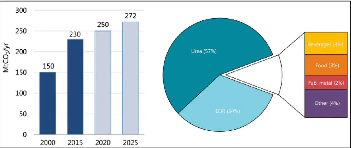
Figure 13 - Growth in global demand of CO2 over the years (left); breakdown of demand in 2015

(right). sources: IEA (2019) [21],. Analysis based on ETC (2018); IHS Markit (2018); US EPA (2018). 13 Figure 14 - Schematic of CO2-EOR and CO2 trapping mechanisms. source: Global CCS Institute [18] 14

Figure 15 – Global storage resource estimates (GtCO2) around the world. Source: Global CCS

Institute, 2019 [18] 16

Figure 16 - CO2 capture technologies [35] 19

Figure 17 - Schematic layout of an IGCC power plant using pre combustion carbon capture[38] 20

Figure 18 - Typical process flow diagram of an oxy-combustion power plant.[41] 22

Figure 19 – Schematic of the Allam (or NET Power) cycle for natural gas (on the left) and coal (on the

right). [42] 22

Figure 20 - Schematic of the chemical looping combustion process. [36] 23

Figure 21- cryogenic distillation Air Separation Unit. [46] 28

Figure 22 - Development over time of energy demand for cryogenic O2 separation [45], [51] 30

Figure 23 - Effect of O2 purity on (a) energy consumption and (b) net lower heating.[45] 30

Figure 24- The dependence of required air flow for the cryogenic module on O2 concentration in the

air (Berdowska and Skorek-osikowska, 2012). 31

(18)

Figure 26 - Experimental data for oxidation of CH4 in a flow reactor as a function of temperature and

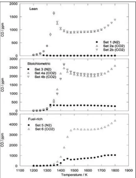
stoichiometry, with N2 or CO2 as bulk gas. [57] 35

Figure 27 - Calculated CO concentration at 300 bar for oxy-combustion (13%v methane, 27%v

oxygen, 60%v CO2). [58] 36

Figure 28 - Calculated laminar flame speed (left), temperature (right) as pressure is varied. [58] 37 Figure 29 - Calculated autoignition delay time (left) and extinction strain rate (right) as pressure is varied. The right graph shows the discrepancy between two chemical kinetic models (Aramco 17 has

been validated at higher pressures). [58] 37

Figure 30 - Borghi diagram. [58] 38

Figure 31 - Conceptual oxy-combustor for CFD modeling using 21 coaxial injectors. [58] 38 Figure 32 - Temperature contours from RANS simulations for case 1 (a) and case 3 (b). [58] 39 Figure 33- Temperature contours (left) and CO mole fractions (right) from LES simulations for case 1

(a), case 2 (b) and case 3 (c). [58] 39

Figure 34 - SCOC-CC cycle schematic. [59] 44

Figure 35 - Allam cycle schematic. [40] 45

Figure 36 - S-Graz cycle schematic (left) and Modified S-Graz cycle schematic (right); [62] 46

Figure 37 - Modified S-Graz cycle schematic. [40] 46

Figure 38 – Revised CES cycle schematic [60], [64] 47

Figure 39 - Supercritical CES cycle schematic. [59] 48

Figure 40 – MATIANT cycle schematic (left) and T-s diagram (right). [65] 49

Figure 41 - E-MATIANT cycle schematic (left;[66]) and T-s diagram (right;[59]). 49

Figure 42 - CC-MATIANT cycle schematic (left) and T-s diagram (right); [67]. 49

Figure 43 - Advanced Zero Emission Power plant (AZEP) cycle schematic [68]. 50

Figure 44 - Zero Emission Ion Transport Membrane oxygen Power (ZEITMOP) cycle schematic (left)

and T-s diagram (right). [69] 50

Figure 45 – Multi criterion decision analysis (MCDA - PESTLE) of the best performing oxycombustion

cycles. [60] 53

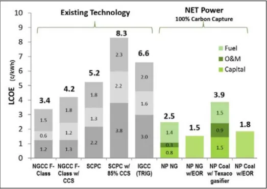
Figure 46 - LCOE for existing technology and LCOE estimation for NET Power technology. [70] 53

Figure 47 - Graz cycle with coal gasification. [71] 55

Figure 48 - Allam cycle with coal gasification schematic. [72], [74] 55

Figure 49 - IGCC SCOC-CC cycle schematic. (adapted from [59] ). 56

Figure 50 - T-s diagram of Rankine cycle; (a) basic, superheated cycle; (b) with reheat stage; (c) with reheat and regeneration; (d) ideal (advanced ultra-) supecritical cycle, with reheat and

regeneration.[80]: 59

Figure 51 - Closed (left) and open (right) Brayton cycle. [81] 60

Figure 52 - Recuperated sCO2 Brayton cycle schematic (left) and T-s diagram (right). [32], [83] 60

Figure 53 - recompression sCO2 Brayton cycle schematic (left) and T-s diagram (right). [32], [83] 60

Figure 54 - Recompression CO2 Brayton cycle efficiency compared to recuperated Brayton cycles with

Helium, nitrogen and CO2. [32] 61

Figure 55 - Cycle efficiency for of a superheated steam cycle, a supercritical steam cycle, a Helium closed Brayton cycle and a recompression sCO2 Brayton cycle in terms of TIT. [83] 63

Figure 56 - Comparison of turbine sizes for steam, helium and CO2. [83], [86] 63

Figure 57- simple recuperative CO2 Brayton cycle; specific turbine (left) and compressor (right)

(19)

VIII Figure 59 - Thermodynamic diagram of CO2 around the critical point, showing constant value lines for

z and fp. [84] 66

Figure 60 - Thermodynamic diagrams of CO2 around the critical point, showing constant value lines

for z and fT. [84] 67

Figure 61 - CP profiles vs. T for different pressures below and above the critical pressure (Pcr) of

CO2.[84] 68

Figure 62 - z and g values around the critical point in the P-H diagram of CO2.[84] 69

Figure 63 - Dimensionless compression work, Wc/Wt, and coefficient mc as a function of the pressure ratio, r, in a pericritical cycle with the compressor inlet temperature at T0,r=0.95 and

T0,r=1.05 (both with a low-pressure value P0,r=1 and a Carnot factor T1/T0=3). [84] 70

Figure 64 - Schematic view of a pericritical regenerative closed cycle; which evolves along two

isobars. Note: If the low-pressure side were below the critical pressure, there would be phase change along part of the low-pressure side, but the scheme of the isothermal lines would be still correct as

they are representing a linearized form.[84] 71

Figure 65 - A schematic view of a pericritical regenerative closed Brayton cycle showing the

additional heats needed, ΔHa, due to the Cp mismatch that appears in the regeneration phase.[84] 72 Figure 66 - ΔT-q diagram (left) and effectiveness of recuperator in recuperative sCO2 Brayton cycle .

[83] 72

Figure 67 - Dimensionless additional enthalpy, ΔHrg/Wt, as a function of the pressure ratio, r, in a pericritical cycle with the low-pressure side at P0,r=1 and the compressor inlet temperatures

T0,r=0.95 and T0,r=1.05.[84] 73

Figure 68 - Dimensionless compression work, Wc/Wt, dimensionless additional enthalpy, ΔHrg/Wt, and thermal efficiency, ηth, as a function of the pressure ratio, r, in a pericritical cycle with the low-pressure side at P0,r=1 and the compressor inlet temperature at (a) T0,r=0.95 and (b) T0,r=1.05.[84]

74 Figure 69 - Dimensionless compression work, Wc/Wt, dimensionless additional enthalpy, ΔHrg/Wt, and thermal efficiency, ηth, as a function of the pressure ratio, r, in a pericritical cycle with high-pressure side P1,r=3 and compressor inlet temperature (a) T0,r=0.95 and (b) T0,r=1.05.[84] 74 Figure 70 - Effects on thermal efficiency of minimum pressure P1,r at a fixed minimum temperature

T1,r and temperature ratio τ [84] 75

Figure 71 - Schematic of the Allam cycle. Adapted from [66] 79

Figure 72 – log(P)-H diagram of the Allam cycle. [90] 81

Figure 73 - Flow diagram of CO2 purification and compression process. [59] 86

Figure 74- Deviation of the EOS from experimental density data for CO2, at four pressure levels in a

relevant temperature range. PR; SRK; Refprop (SW). [88] 87

Figure 75 - Rotor blade with convection cooling, impingement cooling and film cooling (left; from Fu et al. 2005; permission by ASME); stator vane with impingement cooling by inserts and film cooling (right; courtesy of Mitsubishi-Hitachi). Source: course text 'Gas Turbines’ (2018-2019) by T.

Verstraete and E. Dick (UGent).[82] 90

Figure 76 - Temperature contour on rotor blade. [42] 91

Figure 77 - Improved continuous expansion model for turbine cooling. [90] 92

Figure 78 - Characteristics of intermediate turbine stages. [88] 93

(20)

Figure 80 - (Upper left) Test stand for 5 MWth combustor (Toshiba); (Upper right) Rotor of

demonstration turbine (Toshiba); (Lower, centre) Outer casing of Demonstration turbine (Toshiba).

[74] 95

Figure 81- T-q diagram recuperator.[88], [90] 97

Figure 82 - Three scenarios for cooling and heating curves within the recuperator. [88] 97

Figure 83 - Flowsheet of recuperator. Adapted from [90] 100

Figure 84 - Heat exchanger network, recuperator. Allam et al., 2017 (courtesy of Heatric)[74] 101 Figure 85 - Low-temperature section of recuperator. Allam et al., 2017 (courtesy of Heatric) [74] 102 Figure 86 – Net cycle efficiency and net specific work as a function of the combustor outlet

temperature (COT). [90] 104

Figure 87 - – Net cycle efficiency and net specific work as a function of the combustor outlet

temperature (COT), for an uncooled turbine. [90] 105

Figure 88 – Variation of mass flow rates as a function of combustor outlet temperature (COT); mCOOL is the mass flow rate of turbine coolant, mCOM that of the combustor coolant, mCOT is the mass flow rate of fluid entering the turbine and mREC the total mass flow rate of recycled fluid (mass

flow rate at compressor inlet). [90] 106

Figure 89 – Net efficiency as a function of turbine inlet temperature (COT) for various turbine inlet

pressures. [88] 107

Figure 90 – P-H diagram of (a) the Allam cycle and (b) the Allam-Z cycle. [100] 108

Figure 91 - Net efficiency as a function of turbine outlet pressure (MPa). [88] 109

Figure 92 - Net efficiency (solid line) and net specific work (dashed line) as a function of turbine inlet

and outlet pressure (left and right figure respectively). [90] 109

Figure 93 - Recycle compressor (W vap.) and pump work (W den) as a function of TOP (bar). [90] 110 Figure 94 - Specific heat capacity (kJ/kg-C) as a function of temperature for various pressure levels; for the recycle stream, consisting of 97.6%mol CO2. (generated in Aspen Hysys based on the

Peng-Robinson fluid package) 110

Figure 95 - net cycle efficiency as a function of turbine coolant temperature. According to [90] (left)

and [88] (right). 112

Figure 96 - Compressor work (solid line), pump work (dashed line) and net efficiency (dash-dotted

line) as a function of minimum cycle temperature. [90] 112

Figure 97 - Dew point temperature as a function of pressure; for the (dry) recycle stream (97.6%mol

CO2). (generated in hysys) 113

Figure 98 - Net cycle efficiency as a function of isentropic turbine and compressor efficiencies. [90] 115 Figure 99 - Net cycle efficiency as a function of polytropic turbine and compressor efficiencies. [88]

115 Figure 100 - net efficiency for suboptimal cases, with bound values for TIP (bar) and TOT (°C). [90] 117

Figure 101 - Schematic of the Allam cycle. Adapted from [88] 120

Figure 102 - Pressure- specific Enthalpy (P-H) diagram of the Natural Gas Fired Allam Cycle, for the

optimal state found in this study (net cycle efficiency equals 54,44%). 122

Figure 103 – specific Enthalpy - Entropy (H-S) diagram of the Natural Gas Fired Allam Cycle, for the

optimal state found in this study (net cycle efficiency equals 54,44%). 124

Figure 104 - Pressure- specific Volume (P-v) diagram of the Natural Gas Fired Allam Cycle, for the

(21)

X Figure 105 - Temperature- specific Entropy (T-s) diagram of the Natural Gas Fired Allam Cycle, for the

optimal state found in this study. (net cycle efficiency equals 54,44%). 129

Figure 106 - Net cycle efficiency as a function of TIT and TIP, category I. Left: contour-plot; Right: 3D

surface. 132

Figure 107 - Specific work and TOT as a function of TIP for the cases of 1150 and 1200 °C (TIT). 133 Figure 108 - Turbine inlet and - coolant mass flow rates as a function of TIP for 1150 and 1200 °C

(TIT). 133

Figure 109 - Turbine inlet and - coolant mass flow rates as a function of TIT for 250 and 300 bar (TIP). 134 Figure 110 – Total heat content of the turbine exhaust (right axis) and total amount of heat

exchanged in the recuperator (left axis). 135

Figure 111 - 'waste' heat - i.e. hot turbine outlet enthalpy + hot air from ASU enthalpy minus

recuperator duty (referenced w.r.t. 0 °C). 136

Figure 112 – TOT=744 °C ; TIP=250 bar; TIT=1100 °C 137

Figure 113 - TOT=793.3°C ; TIP=250 bar; TIT=1200 °C 137

Figure 114 - TOT=770.1°C ; TIP=250 bar; TIT=1150 °C; Optimal state 137

Figure 115 - Heating curves of all the flows entering the recuperator for the case of 1200 °C (TIT) and

300 bar. 138

Figure 116 - Composite heating curves for the case of 1150 °C (TIT) and 250 bar (TIP). 139

Figure 117 - Composite heating curves for the case of 1200 °C (TIT) and 300 bar. 139

Figure 118 - Recuperator size for the investigated cases (a function of TIT and TIP). 140 Figure 119 - Temperature of the hot streams at recuperator outlet: the air from the ASU compressor

(left) and the turbine exhaust gas (right). 141

Figure 120 - Cold stream pinch point temperature (°C). 142

Figure 121 - Creep rupture strength (MPa) as a function of temperature for various metal alloys (after

10,000 hours of operation). [42] 144

Figure 122 - Nusselt number as a function of Reynolds number for corrugated and smooth pipes.

(source: HRS heat exchangers [101]) 145

Figure 123 - Efficiency as a function of TOT and TIT; computed datapoints marked with a '+'. Left:

contourplot – Right: surfaceplot. 147

Figure 124 - Optimum pressure ratio for all combinations of TOT and TIT; TIP was varied. 148 Figure 125 - Recuperator size (UA – kJ/C-h) and total heat exchanged in the recuperator (kJ/h) as a

function of TOT and TIT. 148

Figure 126 - Net cycle efficiency as a function of TIP and TIT for the case of TOT=740 °C;

T_recycle=720 °C and T_rtc=200 °C. 149

Figure 127 - Net cycle efficiency as a function of TIP and TIT for the case of TOT=740 °C;

T_recycle=720 °C and T_rtc=max. 150

Figure 128 - T_rtc as a function of TIP and TIT; for TOT=740 °C and T_recycle=720 °C. 150 Figure 129 - Net cycle efficiency as a function of TIP and TIT for the case of TOT=740 °C;

T_recycle=735 °C and T_rtc=max. 151

Figure 130 - T_rtc as a function of TIP and TIT; for TOT=740 °C and T_recycle=735 °C. 151 Figure 131 - Individual hot and cold streams exchanging heat in the recuperator, T-q diagram for cases 1 to 3 (T_recycle= 720°C - 735 °C; T_rtc= 200 °C - 511 °C - 395 °C), for the state of TIP=275 bar

(22)

Figure 132 - Hot and cold composite curves for cases 1 to 3 (T_recycle= 720°C - 735 °C; T_rtc= 200 °C - 511 °C - 395 °C), for the state of TIP=275 bar and TIT=1150 °C (1) and 1250 °C (2,3); the respective

optima 152

Figure 133 - Classification of absorption processes for CO2 capture [36], [103] 167

Figure 134 - Schematic diagram of a CO2 absorption plant. [36]. 168

Figure 135 - Principle of a gas separation membrane (a) and a gas absorption membrane.(b) [36]. 170 Figure 136 - Mechanisms for gas permeation through a membrane: (A) Knudsen diffusion. (B)

molecular sieving, and (C) solution diffusion. [41] 171

Figure 137 - A schematic diagram of post combustion carbon capture using Calcium looping . [36]. 172 Figure 138 - Schematic representation of the transport of Oxygen through an ion transport

membrane [41] 174

Figure 139 - Ideal perovskite structure ABO3 [41] 174

Tables

Table 1 - CO2 purity specifications per end use (NETL, 2013). [32] 17

Table 2 - Efficiency comparison of power generation with different carbon capture processes [36] 25 Table 3- Operating conditions and resulting length, time and velocity scales for the three cases

studied. [58] 38

Table 4 - Development index and cycle efficiencies of the reviewed oxy-fuel gas cycles. [59] 41

Table 5 - Performance summary of analysed oxy-turbine cycles. [59] 51

Table 6 - Performance of natural-gas fired oxy-combustion plants. [59] 51

Table 7 - CO2 emissions for each selected cycle [60] 52

Table 8 - Financial performance of oxy-turbine cycles. [59] 52

Table 9 - CAPEX and COE overcost ratio of each selected cycle. [60] 52

Table 10 - Syngas composition vol-% at combustor inlet. [71] 54

Table 11 - coal based power plant performance summary.[59]. 56

Table 12 - Financial results of coal-fired carbon capture.[59] 56

Table 13 - Properties of working fluids considered for closed Brayton cycles.[85] 62

Table 14- Potential applications for sCO2 for power conversion. [32] 76

Table 15 - Fuel specifications – Natural Gas. 83

Table 16 - Average ambient air conditions 83

Table 17 - Key input streams parameter values. 85

Table 18 - Evaluation of EOSs with experimental data. Peng-Robinson; Soave-Redlich-Kwong; Benedict-Webb-Rubin-Lee-Starling. Experimental data ranged from 3.3 - 200 bar; 30 – 420 °C; 0.02-0.43 vol%H2O; up to 0.13 vol% O2; 0.04 vol% N2; and 0.03 vol% Ar. No experimental data was

available on specific heat capacity or enthalpy. [90] 87

Table 19 – Results of the flow-path design of the sCO2 gas turbine. [88] 94

Table 20 - Specific heat of CO2 at 30 and 300 bar for various temperatures. [42] 96

Table 21 - Temperatures and flow rates of recuperator streams. base case [90] 100

Table 22 - Pressure drops in cycle components.[90] 102

Table 23 - Turbomachinery efficiencies. [90] 103

Table 24 - net efficiency for various degrees of CO2 capture and CO2 purity, for an oxygen feed purity

(23)

XII

Table 26 - Optimized cycle conditions reported by [88] 119

Table 27 - Mass flow rates and composition of the flows in the Allam cycle, for the optimal case

found in this study. 127

Table 28 - Parameter values and performance of the case with highest efficiency, for a coolant

temperature of 200 °C and a TOP of 34 bar. 142

Table 29 - Most promising cases found by [90] 143

Table 30 - Optimized cycle conditions reported by [88] 144

Table 31 - Parameter values and performance of the case with highest efficiency, for a TOT of 740 °C

and a recycle stream temperature of 735 °C. 153

Table 32 - Parameter values and performance of the case with highest efficiency, for a TOT of 740 °C and a recycle stream temperature of 735 °C, with optimized distribution of compressor pressure

ratios 154

(24)

List of abbreviations

A list of the abbreviations (LOA) used in this thesis is given, in the chronological order in which they appear in the text.

Chapter 1:

GHG: Greenhouse gas

CCUS: Carbon capture usage and storage TPES: Total primary energy supply TFC: Total final (energy) consumption SOx: Sulphur oxide

NOx: nitrous oxide

CO2: Carbon dioxide

IPCC: Intergovernmental panel on climate change IEA: International energy agency

AR5: 5th_{assessment report (by the IPCC)}

SDS: Sustainable Development Scenario NDC: Nationally determined contribution COP: Conference of parties

UNFCC: United nation framework convention on climate change

Chapter 2:

EOR: Enhanced oil recovery sCO2: supercritical CO2

OOIP: Original oil in place

CPU: Carbon purification and compression unit DAC: Direct air capture

PSA: Pressure swing adsorption TSA: Temperature swing adsorption ESA: Electrical swing adsorption VSA: Vacuum swing adsorption WGS: Water-gas shift reaction

IGCC: Integrated gasification combined cycle SEWGS: Sorbtion enhanced water-gas shift reaction NGCC: Natural gas combined cycle

ASU: Air separation unit EGR: Exhaust gas recirculation CLC: Chemical looping combustion LCA: Life cycle analysis

Chapter 3: Ar: Argon

ITM: Ion transport membrane

CLOU: Chemical-looping Oxygen uncoupling CLAS: Chemical-looping air separation LP-C: Low-pressure column

HP-C: High-pressure column MMM: Mixed matrix membrane OTM: Oxygen transport membrane

CES: Clean energy systems CO: Carbon monoxide

SSME: Space shuttle main burner ICE: Internal Combustion Engine CFD: Computational fluid dynamics LES: Large eddy simulation

RANS: Reynolds averaged navier stokes

IEAGHG: International energy agency greenhouse gas R&D programme

SCOC-CC: Semi-closed oxy-combustion combined cycle

PESTLE: Political, environmental, social, technological, legislative, economic

AZEP: Advanced zero emissions power cycle HRSG: Heat recovery steam generator LCOE: Levelized cost of electricity CAC: Carbon avoidance cost CAPEX: Capital expenditure

USCPC: Ultra-supercritical pulverized coal power plant

SC-PC: Supercritical pulverized coal power plant Chapter 4:

USC: Ultra-supercritical

AUSC: Advanced ultra-supercritical HHV: Higher heating value

PC: Pulverized coal

LTR: Low temperature recuperator PHX: Primary heat exchanger RB: Recuperated Brayton cycle RCBC: Recompression Brayton cycle Tcr: Critical temperature

Pcr: Critical pressure

TIT: Turbine inlet temperature CIT: Compressor inlet temperature Chapter 5:

ASU: Air separation unit

CPU: Carbon purification and compression unit EOS: Equation of state

LHV: Lower heating value EOR: Enhanced oil recovery NG: Natural gas

NIST: National institute for standards and technology REFPROP: Reference fluid thermodynamic and

(25)

XIV

MIEC: Mixed Oxygen ionic and electronic conducting membranes

CMS: Carbon molecular sieve SW: Span-Wagner

BWR-LS: Benedict-Webb-Rubin-Lee-Starling Ni: Nickel

CrMoV: Chrome-Molybdenum-Vanadium (a low-alloy ferritic steel)

TIT: Turbine inlet temperature TIP: Turbine inlet pressure TOP: Turbine outlet pressure TOT: Turbine outlet temperature

MER: Maximum energy recovery – or – Minimum (utility) energy required

HX: Heat exchanger LNG: Liquefied natural gas

COT: Combustor outlet temperature OPT: Optimal

BC: Base case SC: Scaccabarozzi RO: Rogalev

P300: Denoting a case where TIP is equal to 300 bar Chapter 6

CO2: Carbon dioxide

CPU: Carbon purification and compression unit

SRK: Soave-Redlich-Kwong PR: Peng-Robinson ASU: Air separation unit H2O: Water

LHV: Lower heating value Ar: Argon

N2: Nitrogen

IEAGHG: International energy agency – greenhouse gas R&D programme

COT: Combustor outlet temperature TIT: Turbine inlet temperature TIP: Turbine inlet pressure TOT: Turbine outlet temperature TOP: Turbine outlet pressure NGCC: Natural gas combined cycle IEA: International energy agency

IGCC: Integrated gasification combined cycle power plant

BoP: Balance of Plant

HVAC: Heating, ventilation and air conditioning CCS: Carbon capture and storage

EOR: Enhanced oil recovery LCOE: Levelized cost of electricity