Update of risk assessment models for the indirect human exposure

(1)

Update of risk assessment models for the indirect human exposure

M.G.J. Rikken and J.P.A. Lijzen

This investigation has been performed by order and for the account of the Board of Directors of the National Institute for Public Health and the Environment, within the framework of project 601516, knowledge gaps in risk assessment.

(2)

(3)

Abstract

This report describes the research into the methodology of the indirect human exposure models using two risk assessment tools, EUSES and CSOIL. Alternatives are proposed to the methodology of the indirect human exposure models, considering that their validity often remains unclear. The current plant model proved to function as an appropriate exposure route from air and soil to crops. However, improvements such as adding the particle-bound transport to leaves and using separate parameters for roots and leaves are recommended. The two equations describing the indirect exposure via fish seem sufficiently valid. Nevertheless, measured data is uncertain and the equation for hydrophobic substances leaves room for improvement. Large uncertainties for meat and milk are to be expected in the model, especially for hydrophobic chemicals. The method estimating the purification factors for the ingestion of drinking water can be seen as being rough and near worst case in its application. This method must also be updated, preferably with more European experimental data. The ingestion of soil should also include the ingestion of house dust, because part of this dust originates in the soil. In addition to the mentioned improvements, this report proposes further research for the different exposure routes.

(4)

(5)

Samenvatting

In de EU worden verschillende modellen gebruikt om de blootstelling van de mens via de omgeving te schatten. De validiteit van deze modellen is vaak onduidelijk. Dit rapport beschrijft daarom de evaluatie van deze modellen en stelt betere alternatieven voor. Vijf indirecte blootstellingmedia zijn onderzocht: voedingsgewassen, vis, vlees, melk en drinkwater. Een blootsteling aan een chemische stof via de omgeving is indirect als tussen de bron en het moment van blootstelling in ieder geval één overdracht ligt naar enig tussenliggend medium. De directe inname van een stof via de bodem is ook beknopt geëvalueerd. De risicobeoordelingsinstrumenten die zijn gebruikt om de humane indirecte blootstelling te evalueren zijn het Europese Unie Systeem voor de Evaluatie van Stoffen (EUSES) en CSOIL. EUSES wordt gebruikt om de potentiële risico’s van nieuwe en bestaande stoffen te schatten. CSOIL wordt in Nederland gebruikt om voor een woonsituatie de blootstelling aan bodemverontreinigingen te kwantificeren. De resultaten van deze studie kunnen in onderzoekers en risicobeoordelaars helpen met de interpretatie en acceptatie van de indirecte blootstellingroutes en verschaft hen meer informatie voor de discussie over een herziening van deze routes.

Het huidige gewasmodel blijkt geschikt te zijn om de route van lucht en bodem naar de plant te beschrijven. Het model kan nog wel worden verbeterd wanneer het deeltjesgebonden transport vanuit de lucht naar het blad wordt toegevoegd en wanneer voor wortel- en bladgewassen afzonderlijke parameters worden gebruikt. De in EUSES gebruikte groeiperiode is te lang, een kortere periode is beter geschikt. Verder is nader onderzoek gewenst naar het effect van opspattende bodemdeeltjes die op gewassen terechtkomen.

De twee vergelijkingen, die de bioconcentratie in vis beschrijven, schijnen voldoende valide te zijn. Voor hydrofobe stoffen wijken echter de modelberekeningen ernstig af van de experimentele waarden. Hydrofobe stoffen zijn stoffen die een affiniteit hebben voor vet. De vergelijking die wordt gebruikt voor deze stoffen is daarom voor verbetering vatbaar. Het wordt aanbevolen om hiervoor de voorgestelde alternatieve modellen nader te onderzoeken op hun geschiktheid. Het vetpercentage van paling is een factor acht hoger dan die voor vis. Het wordt daarom aanbevolen om te onderzoeken of een aanvullende beoordeling van paling een betere blootstellingschatting kan opleveren.

Bij gebruik van het model dat de concentratie in vlees en melk schat moet rekening worden gehouden met grote onzekerheden. Dit is vooral van belang voor hydrofobe stoffen. Buiten het maximale bereik van de gebruikte vergelijkingen wordt aangenomen dat de concentratie in vlees en melk constant blijft. Door deze aanname overschat het model de berekende concentratie sterk. Het wordt aanbevolen om hiervoor de voorgestelde alternatieve modellen nader te onderzoeken op hun geschiktheid. Verder is het waarschijnlijk beter wanneer de concentraties in vlees en melk worden gerelateerd aan het vetgehalte. Dit omdat het gebruikte vetgehalte voor vlees behoorlijk hoog is en omdat de schatting voor melk geen rekening houdt met vette melkproducten, zoals bijvoorbeeld kaas en boter.

De methode om de zuiveringsfactoren te schatten voor het gebruik van drinkwater is behoorlijk slecht en schetsmatig. De onderliggende database is zeer zwak en is alleen gebaseerd op de Nederlandse situatie. Er moeten meer nationale en internationale gegevens beschikbaar komen om de huidige benadering te actualiseren en te valideren.

Het model voor de humane bodeminname zou ook de inname van huisstof moeten meenemen, omdat een gedeelte van huisstof afkomstig is uit de bodem. Voorgesteld wordt om nader te onderzoeken voor welke stoffen hoge korte termijn blootstelling toxicologisch van belang is. Daarmee kan de opzettelijke en onbedoelde bodeminname worden verbeterd, die vooral van belang is voor kinderen.

(8)

Summary

In the EU, different models are used for the estimation of human exposure to chemicals or substances via the environment. Considering that the validity of these models often remains unclear, a literature search was set up to evaluate them and to look for better alternatives. Five indirect exposure media were examined: crops, fish, meat, milk and drinking water. Exposure to a chemical via the environment is indirect after it has crossed paths with the different media, in which there is at least one intermediate release to any medium between the source and the point of exposure. Direct ingestion of a chemical via the soil was also briefly evaluated. Risk assessment tools used for the evaluation of the human indirect exposure are the European Union System for the Evaluation of Substances (EUSES) and CSOIL. EUSES is used to estimate potential risks posed by new and existing substances to humans and the environment. CSOIL is used in the Netherlands to quantify the residential exposure to substances in the case of soil pollution. The results of this study may help scientists and risk assessors to interpret and accept indirect exposure routes. The study outcome also provides them with more information for fostering the discussion on updates of exposure models. The current plant model proved to be appropriate for the air and soil-to-crops route. However, if a chemical reaches the plant via air, the particle-bound transport to leaves can improve the model. Separate assessment of roots and leaf tissue through use of root and leaf-specific parameter values, can improve the model further. In EUSES, the growing period for crops is too long. A shorter growing period would be more appropriate. The soil re-suspension concept must be examined further, since it could mean a significant improvement.

The two equations describing the bioconcentration in fish seem sufficiently valid. Nevertheless, for hydrophobic substances the model calculations seriously deviate from experimental values. Hydrophobic substances are substances that have an affinity for fat. There is room for improvement therefore in the equation for these substances. The proposed alternatives for eventual replacement of the current approaches should be examined. Since the percentage of fat used for eel is a factor of eight higher than that used for fish, an investigation is proposed to ascertain if an additional eel assessment would give a more accurate estimation.

In applying the exposure model for meat and milk, especially for very hydrophobic chemicals, large uncertainties are to be expected. The concentration in meat and milk is assumed to remain constant outside the maximum range of the equations employed, which may be a great overestimation. Therefore, the proposed alternatives for eventual replacement of the current model should be examined further. It is perhaps better to relate concentrations in meat and milk to fat content, because the fat content of meat used here is rather high, and milk does not represent the much fattier milk products like cheese and butter.

The method estimating the purification factors for the ingestion of drinking water could be seen as being rough and near worst case in its application. The underlying database is very weak, with relevance only to the situation in the Netherlands. More national and international data must become available to update and validate the current approach.

The ingestion of soil should also include the ingestion of house dust, because part of the dust originates in the soil. If the risk of deliberate and inadvertent soil ingestion is to be assessed, substances in soil must be examined to ascertain which of them are toxicologically important at high levels and for short-term human exposure, especially relevant for children.

(9)

1. Introduction

Human direct and indirect exposure

A human risk assessment systematically evaluates the risk posed by the exposure of an individual to a particular substance. One step of a risk assessment is the determination of the exposure. In a human exposure assessment the emissions, pathways and rates of movement of a contaminant or substance are determined in order to estimate the concentration or doses to which human populations are or may be exposed. An exposure is made up of a source (e.g. factory), a release mechanism (e.g. stack), a transport medium (soil, water, air) and an exposure point (eating, drinking, breathing, touching). An exposure is direct, when it occurs to the substance in the transport medium to which it is first released. An indirect exposure occurs to the substance after it has crossed paths with the different media, in which there is at least one intermediate release to any medium or intermediate biological transfer step, between the source and the point(s) of exposure. An example of an indirect exposure path is the consumption of meat from an animal that has accumulated elevated levels of dioxin in its fatty tissue. Estimating the concentrations and intake of drinking water and food products carries out the assessment of the human indirect exposure via the environment. A schematic representation of the indirect exposure routes is presented in Figure 1.

Figure 1 Indirect human exposure routes via the environment.

Objective

The uncertainty in risk assessment can be reduced by implementing solutions for gaps in knowledge, as stated in the objectives of the RIVM project ‘knowledge gaps in risk assessment’. Considering that the validity of the indirect human exposure models often remains unclear, this study was set up to evaluate these models and to look for better alternatives. The strategy used here was a literature search to allow collection of scientific data on indirect exposure routes from the last 10 years. The results of this study may help scientists and risk assessors to interpret and accept indirect exposure routes. The study outcome also provides them with more information for fostering the discussion on updates of exposure models.

Two risk assessment tools are used to evaluate the indirect human exposure routes. One is the European Union System for the Evaluation of Substances (EUSES) and the second is CSOIL. Both models are described briefly in the next paragraph. The EUSES model is used, because

air fish meat dairy products crops drinking water HUMANS soil surface water groundwater cattle

(10)

of its importance for the risk assessment of new and existing substances in the European Union. The CSOIL model describes routes as for instance soil ingestion, which are different from EUSES and significant for specific situations of soil pollution. Other CSOIL routes are similar to those of EUSES, but are described differently. Therefore, also CSOIL is accounted for, because its routes are a useful addition to the ones of EUSES. This study starts from the methods, model concepts and exposure routes implemented in EUSES, which are completed with information about the same exposure routes of CSOIL. Direct exposure routes are not considered, except for the soil ingestion of CSOIL. More details about the exposure routes discussed in this report are listed in Table 1. For each exposure route this evaluation is carried out in the following steps:

1. Search for and selection of relevant scientific information, based on a literature search; 2. Analysis of the studies and reports selected;

3. Comparing the results with the current methods and models of EUSES and CSOIL; 4. Discussion and recommendation for updating or refining the current methodology.

Table 1 Details of (in)direct human exposure routes

Exposure via air:

a) Biotransfer from air to crops

b) Biotransfer via cattle to milk and meat · Direct inhalation of air 1)

· Indirect via crops

Exposure via soil:

a) Biotransfer from soil to crops

b) Biotransfer via cattle to milk and meat · Direct ingestion of soil 1)

· Indirect via crops

c) Direct human soil ingestion (only CSOIL)

Exposure via surface water:

a) Purification of drinking water

b) Biotransfer from surface water into fish

Exposure via groundwater:

a) Biotransfer via drinking water of cattle to milk and meat 1)

b) Direct ingestion of drinking water 1) Not considered in this report

Introduction on EUSES and CSOIL

The computerised risk assessment tool EUSES is designed to facilitate the risk assessment of a broad range of substances (EC, 1996, 2004). EUSES is fully in line with the Technical Guidance Documents (TGD), in which the principles have been laid down for a European Union risk assessment (EC, 2003). EUSES was developed for the quantitative assessment of the risks posed by new and existing chemical substances and biocides to man and the environment. Risks to man pertain to consumers, workers and man exposed through the environment. Risks to the environment include risks to sewage treatment plant populations of micro-organisms, aquatic, terrestrial and sediment ecosystems and populations of predators. EUSES carries out the indirect exposure assessment for the food products root and leaf crops, fish, meat and milk (see Figure 1). The exposure via dermal contact and soil ingestion is not addressed in EUSES, because these routes are only significant for specific situations of soil pollution.

In the Netherlands the CSOIL model has been developed to quantify the human exposure for substances through the different exposure routes, which are important in case of soil pollution. The human exposure is calculated using a standardised scenario based on all

(11)

possible exposure pathways for a residential situation. The exposure routes, implemented in CSOIL, are presented in Figure 2.

SOIL AIR concentration representative SOIL CONTENT PORE WATER concentration distribution over soil fractions transfer-processes direct exposure indirect exposure transport to

SURFACE SOIL GROUNDWATERtransport to deposition onuptake by / VEGETATION dilution in INDOOR and OUTDOOR AIR transport to DRINKING WATER permeation into DRINKING WATER ingestion, inhalation, dermal uptake SOIL inhalation, dermal uptake AIR

intake DRINKING WATER, dermal contact, inhalation

SHOWERING

consumption of VEGETATION

Figure 2 Exposure routes in CSOIL.

In contrast with EUSES, routes such as dermal contact and the ingestion of soil are included in CSOIL. There is a version of CSOIL (CSOIL1995; Van den Berg, 1995) on which the current Intervention Values1 are based and a revised version (CSOIL2000) used for the calculation of risk limits for soil and groundwater (Lijzen et al., 2001). The revised version was developed during a project on the evaluation of the Intervention Values.

Model evaluation

Judgement about a model cannot be made without knowing its purpose. Therefore, EUSES and CSOIL are evaluated to understand the realism of their model concepts relative to the intended purpose. Risk assessment tools as EUSES and CSOIL are used in a regulatory context and have a predictive character, because, with respect to the exposure of substances, there is relatively little known. Both models apply a standard generic scenario for their risk assessment and use simple and generic methods, which results in a conservative point estimate. Naturally, an assessment requires an efficient methodology and it is important to protect humans from possible effects. A worst-case approach may trigger too much false positives. Hence, the indirect exposure routes must deliver suitable results for a reasonable worst-case assessment, indicating a protective approach. The evaluation of the model concepts is not simple, because the conservative estimates are usually not directly comparable to measured data. The degree of deviation from reality can be substantial for the indirect exposure routes, but in each case these routes are evaluated as a compromise between straightforward methods and precise results. In both models a kind of site-specific assessment is possible by adjusting the default data to reach more realistic results of an intermediate (refined) assessment. But, in this report the model concepts are evaluated mainly as a tool for the initial (screening) stage, based on a generic scenario.

1_{Intervention values are generic soil quality standards used to classify historically contaminated soils, sediments}

(12)

Introduction on bioaccumulation

For the indirect exposure routes the methodology estimating bioaccumulation is most important. Bioaccumulation is the process that causes an increased chemical concentration in an organism as a result of chemical uptake through all possible routes of chemical exposure. Bioaccumulation takes place under field conditions and is a combination of chemical bioconcentration and biomagnification (Gobas and Morrison, 2000). Bioconcentration is the increase of the concentration in an organism and is the result of diffusive mass transfer of a contaminant in the environment. Biomagnification is the increase of the concentration in an organism as a result of consumption of contaminated food (Jager and Hamers, 1997; Gobas and Morrison, 2000). Bioaccumulation and bioconcentration are usually expressed in the form of a bioaccumulation factor (BAF) or bioconcentration factor (BCF), respectively, which is the ratio of the chemical concentration in the organism to those in the environment. Biotransformation influences bioaccumulation when chemical substances undergo chemical or biochemical reactions in the organism. The biotransfer factor (BTF) is the ratio between the concentration of a contaminant in animal tissue or an animal product (e.g. meat or milk) and the daily consumption of that contaminant.

There are two general approaches for quantifying bioaccumulation, an empirical and a mechanistic one (MacKay and Fraser, 2000; Schwartz et al., 2000). From an empirical approach the bioaccumulation factor can be deduced from the concentration in the organism and a measured experimental concentration. The more demanding mechanistic approach compiles a mass balance model in which the various uptake and loss processes are quantified. Such models need more data about the chemical and the organism. Empirical models are descriptive, where mechanistic models are more explanatory. As the science of bioaccumulation has progressed, there has been a corresponding shift from the empirical to the mechanistic approach. When bioaccumulation is described in a mechanistic manner, a steady state and a dynamic approach could be distinguished. More information about the mechanisms and models of bioaccumulation can be found in e.g. Gobas and Morrison (2000), MacKay and Fraser (2000) and Jager and Hamers (1997).

Method

The literature search was carried out using the databases Toxline Plus (1991-2001), Current Contents Archives (1997-2003/10/21) and Medline (1989-2003/10). The main entries for the search profiles are presented in appendix 2.

Readers’ guide

In the following four chapters the different human exposure routes are described on the basis of the different human intake media: plants (crops), fish, cattle (meat, milk) and drinking water. The direct exposure route via the ingestion of soil is presented in chapter 6. If applicable, in each of these chapters the model concepts of EUSES and CSOIL are described, followed by an evaluation of the concepts in question. Further, in each chapter alternative model concepts are presented and conclusions drawn. This report ends with a brief description on alternative human exposure routes in chapter 7 and with general conclusions and recommendations in chapter 8.

(13)

2. Plant model

2.1 Model description

2.1.1 EUSES

In EUSES the model settings of a one-compartment steady state model of Trapp and Matthies (1995) are used for calculating the concentration in upper plant parts. The uptake takes place from soil porewater with subsequent translocation and partitioning to upper plant parts and from air by diffusive gas exchange (see Figure 3). All above ground parts are equal and treated as one well-mixed compartment. Only a distinction is made between the root zone and the upper plant parts. The model does not have a fruit compartment and can therefore not be used for fruits, such as cereals. Plants are in steady state with a 180-days average porewater concentration and leaves with an annual average air concentration. Sinks are metabolism and photodegradation, and growth leads to a dilution effect. For calculating the concentration in roots equilibrium approach is used. The equations in the TGD for calculating the concentration in roots are based on the model proposed by Trapp and Matthies (1995). For calculating the concentration in root tissue, the value of the partitioning coefficient between (upper) plant material and water is used. The TGD scenario will provide a kind of average approach, independent of crop type, harvest time or averaging method.

Figure 3 Fate processes accounted for in the plant uptake model of EUSES.

2.1.2 CSOIL

In CSOIL concentrations in plants can be calculated for metals, other inorganic compounds and organic compounds.

In CSOIL1995 measured BCF values are used for metals and, when these are lacking, they are calculated with the equation of Baes et al. (1984), giving a correlation between the BCF value and the soil–water distribution coefficient (Kd). In CSOIL2000 empirical BCF values for all metals from field studies were collected from literature. Based on data for each crop a consumption averaged value was derived for each metal (Versluijs and Otte, 2001). These BCF values are derived for a standard soil in polluted areas.

For other inorganic compounds in CSOIL1995 the concentration in plants (80% water) are assumed to be equal to the soil porewater concentration. Therefore, a fixed BCF value is calculated in CSOIL based on a fresh weight basis as 80% of the soil porewater concentration

air diffusive exchange soil water translocation elimination growth dilution

(14)

(Briggs et al., 1982, 1983; Ryan, 1989). This was not changed in CSOIL 2000, except for cyanides (Köster, 2001).

For organic compounds in CSOIL 1995 the relations of Briggs et al. (1982, 1983) were chosen to calculate the BCF values for the leaf and stem and for the roots of crops. In CSOIL2000 it was chosen to use the one-compartment plant model of Trapp and Matthies (1995) for the calculation in the aboveground plant parts as well as the uptake by roots. In Rikken et al. (2001) a comparison is made between Trapp and Matthies and Briggs. In principal the Trapp and Matthies approach in CSOIL2000 is the same as applied in EUSES, but some modifications were made in the parameters of plant characteristics. For root crops the lipid content and the exponent giving the similarity between octanol and plant lipids are important parameters. Based on the variations given in literature the ‘volume fraction of lipids in plant tissue’ was set at 0.005 (0.01 in EUSES), because the lipid content in roots seem to be lower than for shoots. The ‘correction factor for differences between plant lipids and octanol’ was set at 0.8, because for root tissue a lower factor was found in literature. These modifications are also described in more detail in Rikken et al. (2001). For leafy crops only the plant density was changed (to 800 kg/m3) compared to the use of Trapp and Matthies in EUSES (700 kg/m3). The influence of soil re-suspension was taken into account by assuming that the contribution of soil to the plant concentration is 1% of soil per dry weight plant (see also Trapp et al., 1998).

In CSOIL1995 the deposition on leaves is calculated on the basis of the Hetrick and McDowell-Boyer (1984) equation and is evaluated in Versluijs et al. (1998). In CSOIL2000 this deposition was removed and only soil re-suspension was accounted for (as proposed in Rikken et al., 2001).

2.2 Evaluation of the plant model

2.2.1 Evaluation of model concepts

General observations

Several authors evaluated the plant model of EUSES and CSOIL (Trapp and Matthies, 1995; Jager and Hamers, 1997; Jager, 1998; Schwartz et al., 2000; Trapp and Schwartz, 2000), and all came to more or less the same conclusions.

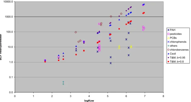
The parameterisations of the equations in the TGD for calculating the concentration in roots or fruit are based on a generic leafy crop and seem to characterise grasses. Especially the properties of grass may be different from regular crops, specifically the leaf area in relation to volume and transpiration rates. Roots have different properties than leaves as for lipid and water content. For an update of the plant model of CSOIL a comparison was made with the calculations based on Briggs and Trapp and Matthies (Rikken et al., 2001). Scarce literature data on the uptake of organic compounds in roots were available. The comparison showed that the Trapp and Matthies model of CSOIL2000 (with adjusted parameters, see paragraph 2.1.2) corresponds more with experimental data than the Briggs model and the unchanged Trapp and Matthies model using a correction factor of 0.95 (see Figure A, Appendix 3). Only the experimental BCF values for roots of chlorobenzenes seem to be higher than the estimated ones. Nevertheless, data are scarce and more data would be necessary to better evaluate the model concept.

In the EU risk assessment, an equilibrium approach is used for the uptake of chemicals from soil into root vegetables. Hence, roots are assumed to be in direct equilibrium with porewater. This assumes a large surface area of several fine roots. The larger roots of root vegetables

(15)

behave quite differently. Trapp (2000) developed a dynamic root uptake model for neutral hydrophobic organic chemicals and compared it with the equilibrium approach. The model considers input from soil and output to stem with the transpiration stream plus first-order metabolism and dilution by exponential growth. He tested the dynamic model against experimental uptake of hydrophobic compounds in carrots. It appeared that measured concentrations in carrot peels were up to 100 times higher than in the core. The equilibrium approach can predict concentrations in the peels, but for carrot cores and for the whole carrot the dynamic model should be preferred. For chemicals with a logKow of lower than 2, there

was no relevant difference between the dynamic model and the equilibrium approach.

The internal regressions (e.g. for the transpiration-stream concentration factor, TSCF) are found to be uncertain for hydrophobic compounds (Trapp and Schwartz, 2000). Jager and Hamers (1997) found the estimation routine for the transpiration-stream concentration factor (TSCF) questionable as there is little correlation with Kow.

It is assumed that plants are growing exponentially, which is only valid if they are harvested before maturation (lettuce). It is not useful for mature plants. When the growth rate decreases well before harvest, an underestimation of the leaf concentration may occur. This underestimation will only be relevant when the half-life in soil is not too low (>100 days) and when the logKleaf-air is larger than 6.

For the partitioning between air and plant the air fraction of the plant is also taken into account. The leaf-air partition coefficient is calculated as the ratio of the leaf-water and air-water partition coefficient. This estimator on the basis of phases in the leaf is generally valid (within a factor of five) (Polder et al., 1997). Schwartz et al. (2000) validated the assumption that plants are in steady state with the annual average air. He determined that 95% of steady state in the standard scenario would be achieved within 86 days.

Deposition and soil re-suspension concept

The particle-bound transport to leaves is ignored in the EUSES model, both for deposition from air and for soil re-suspension. Trapp and Matthies argued that dry and wet deposition are unlikely to contribute significantly to the concentration in leaf. Recent work indicates that this route may be very important for dioxins and similar liphophilic compounds. The generic model yields an underestimation for liphophilic chemicals, which can be reduced significantly by adding the deposition on plant leaves into the model (Chrostowski and Foster, 1996; Jager, 1998; Trapp et al., 1997; Ballschmiter et al., 1996). Meneses et al. (2002) developed a model to predict the distribution and transport of hydrophobic chemicals such as PCDD/F from the air to vegetation. With respect to the different pathways, in decreasing order of importance the vapour-phase absorption (±66%), wet particle deposition (±21%), dry particle deposition (±13%) and uptake by roots contribute to PCDD/F concentrations in plants. The deposition of particles on leaves is described in Trapp and Matthies (1998) as a part of the CemoS risk assessment framework. The uptake is modelled with the estimated particle fraction (Junge, 1977), wet and dry deposition velocity, leave area and concentration in air. The sinks are growth dilution and weathering. Lorber and Pinsky (2000) described the particle-phase portion of the EPA air-to-plant model. The total deposition of the EPA model is simply modelled as the particle-bound air concentration times a deposition velocity. The deposition velocity of 0.20 cm/s of the EPA model was found to be too rapid. With the velocity of 0.20 cm/s, deposition amounts were about 3 times higher than measured. Average velocities of 0.06 – 0.08 cm/s were calculated for a rural and industrial site, respectively. Schwartz et al. (2000) determined the uncertainties in estimating the particulate fraction as described in the TGD. The estimation will significantly improve if alternative values for the

(16)

surface area of aerosol particles and the constant of Junge equation are used instead of the TGD defaults.

The importance of soil re-suspension for EUSES was not evaluated. Trapp and Schwartz (2000) argued that, because of the exclusion of the particle-bound transport, the model would likely not give valid results for very hydrophobic compounds. The transfer by re-suspension of soil particles (rain splash) is of importance for deep-growing parts of plants that show a funnel-formed shape, e.g. lettuce (Schwartz et al., 2000; Rikken et al., 2001; Jager, 1998). Soil and dust particles can deposit on the different plant parts by rainsplash. A value of 30 g dry soil per kg dry plant (= 3%) for soil attached to crops is based on a mean estimated soil load on plants as in Sheppard and Evenden (1992). This value is based on the attached soil that cannot be removed by normal food preparation. Trapp and Matthies suggest a less conservative value of 1% dry soil per dry plant. Rikken et al. (2001) concluded that the rainsplash or soil re-suspension concept should be added to CSOIL, setting the contribution of this route at a provisional value of 1%.

Studies and reports evaluating several plant models

Schwartz et al. (2000) compared the simple approach of applying bioconcentration factors (Briggs et al., 1983, Travis and Arms, 1988) with the model of Trapp and Matthies for dioxins and PCBs. The use of bioconcentration factors leads to a significant underestimation of about two orders of magnitude. The Trapp and Matthies approach achieves a good correspondence to measured values for chemicals in the gaseous phase. The Trapp and Matthies approach results in better estimations compared to the bioconcentration factors, although the measured values are underestimated for stronger particulate-bound dioxins. All in all, the Trapp and Matthies approach represents a good compromise between complexity and the accuracy of its estimations, but it can be improved by the integration of further processes such as the deposition of particles.

McLachlan (2000) compared four estimation methods for deriving the plant-air partitioning coefficient. The approaches were the linear method, non-linear method (Trapp and Matthies, 1995), two-compartment method (Riederer, 1995) and the Müller et al. method (1994). In summary, current methods agree well with each other. The results indicated good agreement among the four methods for predicting the plant-air partitioning coefficient of lindane, anthracene and 2,2’,5,5’-tetrachlorobiphenyl in grass. McLachlan (2000) did not present a ranking of preference, only that the compared methods can at best give only an approximate value of the plant-air partitioning coefficient. The potential error associated with these methods is more than an order of magnitude. He concluded that much more research is required for an understanding of the influence of both the physical-chemical properties and the temperature on the plant-air partitioning coefficient.

Lorber and Pinsky (2000) evaluated three empirical air-to-leaf models for polychlorinated dibenzo-p-dioxins and dibenzofurans. The vapour deposition model of Trapp and Matthies (1995) significantly underestimated the grass concentrations by a factor of more than 10. The EPA model (US EPA, 1994) performed the best of the three models tested, because it came the closest to the grass concentrations at the test sites, within a factor of two at the rural site. The EPA model performed better because, besides the vapour phase, it also accounts for the particle-phase.

For an update of the plant model of CSOIL a comparison was made between the calculations based on Briggs and Trapp and Matthies (Rikken et al., 2001). Scarce data were available for

(17)

the uptake of contaminants in aboveground plant parts. In general the experimental BCF values for the aboveground plant parts were higher than calculated with Briggs or with Trapp and Matthies (see Figure B, Appendix 3). Compounds with a lower octanol-air partition coefficient (Koa; see McLachlan, 2000) are more volatile and have lower BCF values. In

contrast with the Briggs model, the comparison made clear that the Trapp and Matthies model takes the volatility into account. Also the contribution of soil re-suspension (1% on dry weight basis) was added to the estimated BCF values of Trapp and Matthies, which seemed to give a better fit compared to the measured concentrations. More data would be needed, especially on the influence on soil re-suspension to further improve the model concept in CSOIL.

Meneses et al. (2002) looked closely to the distribution and transport of polychlorinated dibenzo-p-dioxins and dibenzofurans (PCDD/F) from air to soil and vegetation. They found the vapour-phase absorption the most important pathway. They concluded that the models of Trapp and Matthies, Hung and Mackay and McLachlan predict the vegetation levels in a good agreement with the measured levels. The results of all models showed the same trend. For almost all low-substituted congeners of PCDD/F the concentrations in vegetables were calculated lower than the measured ones. For most high-substituted congeners the model estimations were higher than the measured values.

Freyer and Collins (2003) evaluated nine plant uptake models against experimental data. These models ranged from simple deterministic equilibrium and steady state risk assessment screening tools to more complex dynamic models that considered physical, chemical and biological processes in a mechanistic manner. One of the compared models was the Trapp and Matthies (1995) model that is used in EUSES. Among the equilibrium and steady state models, the Trapp and Matthies (1995) model appears to overestimate most significantly the foliage concentration factor in the water uptake scenarios. In the soil uptake scenarios the Trapp and Matthies (1995) model produced a BCF closer to the experimentally derived values than in the water uptake scenarios. The most probable cause for this difference is the longer exposure duration of the soil uptake scenario, where equilibrium conditions are more likely established. This could mean that equilibrium and steady state models should be more accurate for experiments with a longer duration. The predictions of the dynamic, equilibrium and steady state models proved to be highly similar for modelling the air uptake, but the dynamic model of Paterson and Mackay (1994) performed probably the most accurate of all. Freyer and Collins (2003) concluded that for the purpose of more chronic exposure duration (in terms of weeks) at the screening stage of the risk assessment the steady state Trapp and Matthies (1995) model proved to be sufficient. However, it will prove necessary to use a more complex dynamic model if a chemical reaches the plant via the aerial uptake route, because the exposure duration is relatively short in this rapidly changing medium and the source term is not constant.

2.2.2 Evaluation of model parameters

The 180 days growing period is too long (Jager and Hamers, 1997). A period of 50 days (lettuce) and 120 days (cabbage) is more appropriate. For root crops 140 days (potato) and 150 days (carrot) is more likely. According to Jager and Hamers (1997) the 180 days period is wrong for crops, but may be used when the following is kept in mind. The TGD approach will overestimate concentrations in root crops and long growing leaf crops (e.g. cabbage) when the chemical’s half-life in soil is short. At short half-life periods in soil (20 days) and logKleaf-air >6, the TGD approach will underestimate levels in short-growing crops (e.g.

(18)

lettuce) by a factor of two. When the half-life in soil is larger than 100 days and logKleaf-air >6,

the assumption of continuous growth becomes crucial for long-growing crops and it is better to use actual time-related growth information.

In EUSES the parameter values for a generic crop are used which are equal for root and leave crops. The generic crop seems to characterise grasses (Schwartz et al., 2000). Trapp (2002) determined root specific values for the lipid content, the water content and the empirical correction factor for differences between plant lipids and octanol. Trapp used a lipid content for roots tissue of 0.025 g/g and a water content of 0.89 g/g. The current empirical factor of 0.95 is applicable to leaves (Briggs et al., 1982), the value for roots is 0.77 (Briggs et al., 1982; Trapp, 2002). Jager and Hamers (1997) also advised to use root and leave specific properties in stead of the generic parameters. The current EUSES parameters and the proposed ones are presented in Table 2.

Table 2 Proposed parameters for the plant model (Jager and Hamers, 1997; Trapp, 2002)

EUSES Proposed Unit Plant leaves

Volume fraction fat 0.01 0.01 m3.m-3

Volume fraction water 0.65 0.65 m3.m-3

Volume fraction air 0.30 0.30 m3.m-3

Bulk density tissue 700 800 kgwwt.m-3

Empirical factor 1) 0.95 0.95

-Plant roots

Volume fraction fat 0.01 0.005 m3.m-3

Volume fraction water 0.65 0.93 m3.m-3

Bulk density tissue 700 1000 kgwwt.m-3

Empirical factor 1) 0.95 0.77

-1) Empirical correction factor for differences between plant lipids and octanol.

A constant environmental temperature of 12ºC is assumed, which is an additional source of uncertainty since plants mainly grow in spring and summer (Schwartz et al., 2000).

2.3 Alternative models

Paterson and Mackay (1994) developed a dynamic three-compartment mass balance model of a plant to quantify the uptake of organic chemicals from soil and atmosphere. The three compartments are roots, leaves and remaining structure, which is mainly stem, but could also include fruits, seed or tubers. The processes involved are diffusion and bulk flow of a chemical between soil and root, transport within the plant in the phloem and transpiration streams between root, stem, and exchange between foliage and air and soil and air. The model accounts for metabolism and growth. The model is used widely and has been tested against field data. The model predictions are generally good.

Freyer and Collins (2003) evaluated nine plant uptake models against experimental data and found the Paterson and Mackay model to perform probably the most accurate of all for modelling the air uptake. Nevertheless, the model is relatively complex and therefore Hung and Mackay (1997) simplified it to develop a model containing only readily available parameters. The results of the simplified version compared well with both the experimental results and the results of Paterson and Mackay (1994). The Paterson and Mackay (1994) model can better simulate actual transport processes and is recommended for research processes (Hung and Mackay, 1997). The simplified Hung and Mackay (1997) model is more appropriate for risk assessment purposes.

(19)

Chrostowski and Foster (1996) developed a methodology for assessing plant uptake of hydrophobic chemicals (as PCDDs or PCDFs) via air, by analysing the vapour:particulate partitioning behaviour of those compounds. This methodology incorporates physico-chemical properties and photolytic degradation rates and applied them to assessing environmental concentrations associated with uptake of vapour phase chemicals in plants. Chrostowski and Foster found one major shortcoming of other models that describe the air uptake of plant. They only take volatilisation into account as an elimination process and do not reflect the photolysis that is likely to occur for PCDDs or PCDFs.

ECETOC (1995) and Schwartz et al. (2000) described the molecular connectivity index (MCI). The MCI is an index derived from the molecular structure. In more detail the MCI is described in section 3.3. Dowdy and McKone (1997) described the MCI for predicting the plant uptake of organic chemicals. They used for the first-order MCI the index 1χ for the sum of bond values of atoms over the entire molecule and a correction factor for the polar fragments of chemicals. Dowdy and McKone used only one order of χ, in contrast with Lu (1999, 2000), who used several orders of χ for predicting bioconcentration factors in fish (see section 3.3). Dowdy and McKone compared the predicted uptake of the MCI with experimental values and relative to the Kow-approach. The results indicate that the MCI

performs significantly better than Kow as a predictor of the bioconcentration from soil to

above-ground plant tissues and performs only slightly better as a predictor of the bioconcentration from soil solution to below-ground plant tissues. For predicting the bioconcentration from air to plant tissues the MCI was accurate but less precise and had limited validity relative to Kow. With regard to bioconcentration in plants, the data sets were

very small (n≤14) and therefore more experimental measurements were needed to improve the existing models. Compared to the Kow-approach, MCI does not have as much inherent

uncertainty due to measurement and estimation errors. With the Kow-approach experimental

procedures are required to determine a Kow value. Therefore, MCI is faster because it is not

linked to experimental procedures. MCI has a large potential for reliably estimating the BCF of new substances and has few limitations in its use. MCI is a relatively complicated method, compared to the logKow-approach, for which more substance information is needed to

calculate the χ-value and the polar correction. The main disadvantage is that the validation of the method is limited and not (yet) broadly applicable.

The Trapp and Matthies model does not have a fruit compartment and can therefore not be applied to fruits. Trapp et al. (2003) developed a steady state fruit tree model for uptake of organic compounds from soil. It considers xylem and phloem transport to fruits through the stem. The calculated values were compared to measured values that originate from two different studies. To verify or to falsify the model predictions, field measurements or experiments are needed.

The EU chemical risk assessment uses a plant uptake model that is exclusively developed for neutral compounds. Trapp (2000) modelled the uptake in roots and subsequent translocation of ionisable organic compounds. The model approach combines the process of hydrophobic sorptions, electrochemical interactions, ion trap, advection in xylem and dilution by growth. The model needs more input data such as the pKa and valency number of the compound and the pH and chemical concentration in the soil solution.

(20)

2.4 Conclusions

- The steady state Trapp and Matthies (1995) model proved to be appropriate for the screening stage of a risk assessment. Nevertheless, the Hung and Mackay model (1997) seems a promising alternative for risk assessment purposes. A direct comparison between the Hung and Mackay model and the Trapp and Matthies model has not been performed and therefore it is advised to evaluate both models against experimental data.

- The Trapp and Matthies (1995) approach could be improved by adding the particle-bound transport to leaves if a chemical reaches the plant via air.

- The EUSES approach could further be improved by separately assessing roots and leave tissue, in stead of the current generic crop approach. Root concentrations can be predicted more accurately using the described root specific parameters. An evaluation against experimental data is advised to determine whether the dynamic root uptake model of Trapp (2000) could be a significant improvement.

- Research is recommended to find out whether the following could deliver a better estimation:

A separate assessment of fruit e.g. with the steady state fruit tree model of Trapp et al. (2003);

An adjustment of the 180 days growing period, because this period is too long. A period of 50 to 120 days (lettuce, cabbage) for leaf crops and 150 days (carrot) for root crops is more appropriate;

The soil re-suspension concept;

(21)

3. Fish model

3.1 Model description

3.1.1 EUSES

In EUSES the concentration of chemicals in fish is predicted with a bioconcentration factor (BCF). The BCF is determined by the ratio of uptake and elimination rate, based on a two-compartment model of fish and the surrounding water. The BCF is founded on a logKow

-approach with two regression equations. A simple linear model of Veith et al. (1979) is used for chemicals with a logKow range of 1 to 6. For substances in the logKow range of 6 to 10 a

parabolic equation is applied (Connell and Hawker, 1988). For chemicals outside the logKow

range of 1 to 10, the BCF is calculated with the minimum or maximum logKow of that range.

The model assumes that fish will reach equilibrium with the annual average dissolved water concentration. The chemical’s concentration in fish is in a steady state and the growth of fish is neglected. A further assumption is that the bioconcentration factor can only be derived from the lipophilicity of the substances and that the substances are only enriched in the lipid fraction of the organism.

3.1.2 CSOIL

The human exposure via the ingestion of fish is not considered in CSOIL.

3.2 Evaluation of the fish model in EUSES

3.2.1 Evaluation of model concepts

Mackay and Fraser (1982, 2000) examined the data of Veith et al. (1979) and argued that the slope of 0.85 of the regression equation was not significantly different from 1.0 and that the simpler one-parameter relationship applies. Therefore the regression equation could be simplified as logBCFfish = logKow – 1.32 or BCFfish = 0.048 · Kow. The resulting correlation

coefficient was similar to that obtained by Veith et al. (1979).

Devillers et al. (1996) compared several BCF models based on logKow, including the models

of Veith et al. (1979) and Connell and Hawker (1988). The comparison was performed for a data set constituted of 436 experimental BCF values recorded for 227 chemicals. The study showed that for chemicals with a logKow<6, the different models yielded equivalent results.

For highly hydrophobic chemicals with a logKow>6, the bilinear model of Bintein et al.

(1993) was superior to the other models, including the Connell and Hawker model.

Jager and Hamers (1997) found the assumption that fish will reach equilibrium with the water concentration a reasonable one. They demonstrated that equilibrium with the annual average water concentration is comparable to the annual average concentration in a dynamically modelled fish. They found the validity of the parabolic equation (logKow>6), as advised in the

TGD, questionable, because it may result in a serious underestimation of the BCF for hydrophobic compounds. It may be better to assume a constant BCF at logKow>6.

Jager (1998) concluded that the two QSARs seems sufficiently valid for use in EUSES, as a compromise for the screening phase of a risk assessment. The variation remains large for

(22)

very hydrophobic compounds. This is demonstrated by the uncertainty in the BCF of 20 for the logKow range of 1-6 and of 185 for the logKow of 5-10 (Jager et al., 1997).

According to Devillers et al. (1998) the simple linear model of Veith et al. (1979) tends to overestimate the BCF values for hydrophobic compounds. From a risk assessment point of view it introduces a recommendable margin of safety for chemicals that are of environmental concern. From a modelling point of view this strategy is highly questionable, because it does not simulate at best the characteristics of the data. He found the equation from Veith et al. (1979) could only be used for chemicals with a logKow<6. Devillers found the results of the

parabolic model (logKow>6) of poor quality and the model has been derived from a limited

set of chemicals. Nevertheless, it allows a better estimation of the BCF for hydrophobic chemicals than the linear model.

Schwartz et al. (2000) presents a list of assumptions of the regression equations for estimating the bioconcentration for fish that are used in EUSES. If all these assumptions hold, the model seemed to deliver suitable results. The used regression equations must be considered as a compromise for the screening phase of the risk assessment. Nevertheless, the model for fish should be used with caution for high Kow values, because of the weak database

and relatively high experimental uncertainties. The results for hydrophilic compounds are within a factor of 10 compared to measured data (Schwartz, 1997). Higher chlorinated PCBs seemed to be underestimated and PCDDs, DEHP and HHCB overestimated. The deviations for hydrophobic compounds were up to a factor of 1000. If an error of approximately two orders of magnitude is acceptable than the results will be sufficient for hydrophobic compounds.

The EUSES model for fish was elaborated for freshwater fish, actually forbidding its application to a marine environment (Schwartz et al., 2000). Therefore, the model must be used with care for marine fish. The bulk of the consumed fish is retrieved from the marine water environment and not from the fresh water environment. This contradiction must be examined further in future.

3.2.2 Evaluation of model parameters

For the generic fish as consumed by humans and predators, a fat content of 3 vol% is used. This is a representative value for most freshwater species. The fat percentage for eel however is a factor of eight higher. Therefore, Jager and Hamers (1997) and Jager (1998) proposed to consider eel separately in the risk assessment.

Furthermore, the model should not be used for compounds with a molecular weight of more than 700 g/mol, because the underlying relationship does not consider such heavy molecules (Schwartz et al., 2000).

(23)

3.3 Alternative models

3.3.1 Empirical models

Many of the empirical relationships tend to break down when dealing with very hydrophobic chemicals (e.g. Connell and Hawker, 1988 or Bintein et al.,1993). According to Mackay and Fraser (2000) and Gobas and Morrison (2000) it is necessary to specify that the BCF is deduced from the dissolved rather than the total aqueous concentration. If the total concentration is used, the BCF will depend on sorption conditions in the water, which are unrelated to uptake and clearance by the organism. An unnecessary variability is introduced into the interpretation of BCFs by using the total concentration in water. The use of the freely dissolved concentration in water is particularly important for very hydrophobic chemicals (logKow>5), which exhibit high tendency to associate with organic matter in the water. Many

regression models show a drop at high Kow values. The bioavailability is neglected by using

the total concentration in water. Another reason for the drop at high Kow values can be found

in the insufficiently long test duration time. It is not always possible to conduct tests for an adequate time period while maintaining constant exposure conditions. In tests with high Kow

substances (logKow>5), organisms eliminate these substances slowly and therefore the steady

state is also archived slowly.

Bintein et al. (1993) have proposed a non-linear correlation in which the bioconcentration reaches a maximum and then falls above logKow of 6. The fall above logKow of 6 is

presumably a result of reduced bioavailability. Devillers (1998) found that the Bintein et al. (1993) gives good simulation results, and that the model presents a large logKow domain of

application. Further, he found the Bintein model the most flexible one for taking into account experimental artefacts and for integrating numerous abiotic and biotic constraints linked to BCF data. For screening purposes this model can be favoured more than the parabolic equation of Connell and Hawker.

Meylan et al. (1999) have proposed a more detailed method of predicting bioconcentration factors from Kow. It is believed that the discrepancies which exist between the predicted

BCF’s from the derived empirical relationships and those observed in the environment are partly due to the relatively small data sets used in the past studies. In Meylan 694 chemicals were grouped and analysed which resulted in several correlations for non-ionic and ionic compounds, including correction factors for the BCF estimation of several compound classes. For both groups of compounds the proposed equations resulted in a higher correlation coefficient than for equations established in other empirical models as Veith et al. (1979) and Bintein et al. (1993). The equations of Meylan have the advantage that they are based on a large data set with a wide range of Kow, it allows for metabolic conversion and it can be used

ionic compounds. The model also predicts the observed reduction in BCF for non-ionic compounds when the logKow exceeds 7. There are also disadvantages, which are bound up

with empirical models. Often there is an uncertainty about the Kow for a compound and

therefore the assigned BCFs can be different. The Kow is also pH dependent for ionising

compounds. There is no mechanistic treatment of bioavailability. For screening purposes this model can be preferred.

ECETOC (1995) and Schwartz et al. (2000) described the molecular connectivity index (MCI). The MCI is a non-empirical parameter that is derived from the molecular structure

(24)

only and has been demonstrated correlating to many physiochemical properties including, water solubility, Kow and Koc. Although the MCI is a non-empirical parameter, the

relationship that correlates it to the BCF is an empirical one. The underlying idea of this method, in its most simple form, is to count the bonds of the hydrogen-suppressed molecular skeleton and to derive an index from them. Hence, the index is based on the structure of the molecule and is proved to correlate with the size, number of branches, volume and surface area of a molecule. The index correlates to experimentally determined biotransfer factors and can serve as a surrogate for a Kow based correlation. In 1995, ECETOC mentioned that the

method is still under investigation and more work is required. Especially, it was necessary to check whether this method is valid for classes of molecules that have not yet been taken into account. More recently, in two studies Lu et al. (1999, 2000) investigated the MCI method for a wide range of non-ionic organic substances (80 and 239 compounds). The MCI estimations were as good to the monitoring data as archived with the Kow-approach. MCI

could be described as more flexible, because it can be computed directly from the structure of organic compounds (Lu et al., 1999, 2000). MCI is also able to reduce uncertainties that are concealed by the deterministic calculations and, thus, offers another advantage with regard to the Kow based method (ECETOC, 1995). MCI were found to be good descriptors of BCF for

non-polar compounds, but not for polar ones (Lu et al., 2000). MCI has a large potential for reliably estimating the BCF of new substances and has few limitations in its use. Compared to the Kow-approach MCI does not have as much inherent uncertainty due to measurement

and estimation errors and is faster, because it is not linked to experimental procedures. The main disadvantage is that this method is not properly validated and not (yet) broadly applicable. Further, the MCI is a calculated variable for which more substance information is needed to calculate several orders of χ-values (i.e. number of atoms and branches of a molecule or molecular surface area). Therefore, MCI is a relatively complicated method, compared to the logKow-approach. More information is necessary to investigate the MCI

more closely.

The critical micelle concentration (CMC) is the concentration of a substance at which micelles (a submicroscopic aggregation of molecules) are formed. As such, the CMC of a substance may provide an alternative method of expressing that substance’s lipophilicity and may also be able to indicate the potential of a substance to bioconcentrate. The CMC is measured by monitoring the change in surface tension of an increased concentration of the substance in water. Above the CMC the surface tension will no longer alter. Few studies are available reviewing the relation of the CMC and bioconcentration. A review by Tolls and Sijm (1993) showed that there was some evidence of increasing bioconcentration with decreasing CMC. However, the data set used included non-steady state studies, as a result of which the authors were unable to conclude that a clear relationship did in fact exist (ECETOC, 1995). Recent studies describing bioconcentration (e.g. Jager and Hamers, 1997; Schwartz et al., 2000; Mackay and Fraser, 2000) did not further mention the CMC method as a serious alternative and therefore it was found unnecessary to investigate this method more closely.

3.3.2 Mechanistic models

The last decade several authors developed and looked more closely to more complex mechanistic models, integrating bioconcentration, biomagnification, growth and elimination. Gobas and Morrison (2000) distinguish three types of mechanistic models: kinetic models, physiological models (i.e. PBPK) and foodweb bioaccumulation models.

(25)

Jager and Hamers (1997) investigated a kinetic model suitable for considering bioconcentration, metabolism and growth. The model describes the partitioning between fish and water and is based on the volume fractions of water and lipids in the fish. Other constituents of the fish are assumed to have no affinity for the chemical. Metabolism and growth dilution can be important for very hydrophobic chemicals and are described by kinetic rate constants. The model also uses rate constants for diffusive uptake and elimination, which can be estimated according to Sijm et al. (1995). The results of this model are comparable with the EUSES approach up to a logKow of 7. For higher logKow values the

BCF remains constant. The authors found this model to predict BCF values satisfactory for most chemicals and the best option for risk assessment, considering the background of the calculated bioconcentration factors and theoretical considerations. Neglecting biotransformation and the effect of molecular size leads to a reasonable-worst-case estimation. The advantages are that the underestimation of the BCFs at high Kow values, as

described in the TGD, is lacking and it makes a discussion on the data set to be used for the regression redundant (each new data set will provide a different regression). Another plus-point is that the effect of growth dilution and chemical specific metabolism rates can be included. The disadvantage of the model is the use of a generic fish, to overcome the increased data requirements as the weight, lipid and water content of fish and the growth and metabolism rates. It is further questionable if this model is applicable for the screening stage of a risk assessment (Schwartz et al., 2000).

Thomann (1989) and Gobas (1993) have developed physiologiclly based kinetic models, including rate constants for chemical uptake and elimination based on physiological parameters (i.e. gill ventilation, feeding, chemical assimilation). Both models are used widely and have been tested against field data. The model predictions are generally within a factor of two to three of the observation made in the field, which can be regarded as acceptable (Gobas and Morrison, 2000).

The physiologically based kinetic model of Thomann (1989, 1992), that considers biomagnification and the organism’s rank in the food chain, explained the increasing error in predicting the BCF with an increasing degree of lipophilicity. The Kow is used to describe the

tendency of chemicals to partition into the lipid compartments of the organisms. The model consists of five biological compartments, including benthic organisms. Four contaminant exposure routes are considered: ingestion of particulates and phytoplankton and ventilation in overlying and interstitial waters. For the simple lipid partitioning of a chemical into an organism the growth of the organism is recognised by the model. For generic growth rates across a simple food chain, the model calculations indicate that field logBCF values could be expected to be at a maximum of about 5.5 at a logKow of about 6. Subsequent increases in

Kow do not result in proportional increases in BCF, because of growth and transfer efficiency

effects. After a value of approximately 6.5 the BCF begins to decline. Below logKow of 5,

decreased uptake and increased excretion prevent food chain buildup.

The steady state food web bioaccumulation model of Gobas (1993) was developed to estimate bioconcentration factors, biomagnification factors, bioaccumulation factors as well as concentrations and fugacities in phytoplankton, zooplankton, benthic invertebrates and fish species in water and sediments. The model uses rate constant to describe the considered processes for organisms of a defined food web. The model estimates the intake of chemical from the gills and the diet and the rate of elimination via gills, faeces, growth and metabolic transformation. The excretion rate constant is set at approximately 25% of the dietary uptake rate constant. Bioavailability is also considered. The model can be applied to many aquatic food webs and uses a relatively small set of input parameters. The uptake efficiency remains constant as logKow increases, until a value of about 6 or 7 is reached after which the uptake

(26)

efficiency decreases. The model was applied to a Lake Ontario food web and yielded satisfactory results, despite the relatively small number of required model input parameters (Mackay and Fraser, 2000). The 95% confidence interval of the ratio of observed and predicted concentrations of persistent organic chemicals is a factor two to three. The EPA has reviewed the model in 1994 and applied it in its Great Lakes Water Quality Initiative (Gobas and Morrison, 2000).

The advantage of this relatively simple model is the consideration of further processes, including feeding interactions, that may improve the results. The weakness of the Thomann and Gobas models is that they treat only a single organism per trophic level (Mackay and Fraser, 2000). Due to its required database the models are considered not practical for the screening stage of a risk assessment.

The steady state fugacity-based bioaccumulation model of Campfens and MacKay (1997) quantifies trophic transfer in aquatic food webs and is a further development of Clark et al. (1990). The model contains a dietary preference matrix containing a number of organisms where each organism can feed on all of the others including its own species. The uptake of contaminants can be from exposure to either water, sediment or pore water. The clearance mechanisms include respiration, excretion, metabolism and grow dilution. The model uses a number of values to describe the transport processes and mechanisms, in terms of fugacity factors, involved in contaminant uptake and release. The use of fugacity factors has the advantage that that ratios are similar for compounds with similar Kow. They are also easily

understandable in terms of equilibrium status in the organism relative to the environment and the associated prey. The results were found to be within a factor of three of the observed values, despite being a relatively simple model in terms of the number of required parameters (Mackay and Fraser, 2000). Nevertheless, because of its complexity this model is not preferred for screening purposes.

3.4 Conclusions

- As a compromise for the screening stage of a risk assessment the two regression equations of EUSES seem sufficiently valid.

- Nevertheless, the parabolic equation of Connell and Hawker leaves room for improvement. This equation was often qualified as questionable, because serious deviations were calculated for hydrophobic compounds. Therefore, it is recommended to examine alternative approaches for replacing the current approach of Connell and Hawker.

- The empirical models of Bintein et al. (1993), or perhaps better, of Meylan et al. (1999) seem good alternatives.

- The mechanistic model of Jager and Hamers (1997) seems also to be a good alternative, although Mackay and Fraser (2000) and Schwartz et al. (2000) do not prefer mechanistic models as an alternative approach for screening purposes. Using a generic fish largely circumvents the disadvantage of the increased data requirements.

- Since the percentage of fat used for eel is a factor of eight higher than that used for fish, an investigation is proposed to ascertain if an additional eel assessment would give a more accurate estimation.

(27)

4. Meat and milk model

4.1 Model description

4.1.1 EUSES

In EUSES the Travis and Arms (1988) log-linear geometric mean regression equations on experimentally derived bioaccumulation factors and the logKow are used. A schematic

representation of the indirect exposure routes for cattle is presented in Figure 4. The bioaccumulation factors are calculated for fresh meat and milk. The bioaccumulation factor for meat was derived from data on 36 organic compounds, with a logKow of 1.5 – 6.5. The

bioaccumulation factor for milk was derived from data on 28 organic compounds, with a logKow of 3.0 – 6.5. Outside these ranges, the minimum or maximum Kow is used. To obtain

the concentration in meat and milk, the bioaccumulation factors are multiplied by the concentrations and uptake rates for grass, soil, air and drinking water.

Figure 4 Uptake routes for cattle accounted for in EUSES.

4.1.2 CSOIL

The consumption of meat and milk is not described in CSOIL2000, because these routes were considered not relevant for a local site-specific assessment in the Dutch situation. Therefore, these routes are not taken into account for deriving intervention values for the human exposure. In 2002 these routes were added to CSOIL for deriving soil-use specific objectives for agricultural areas (Van Wezel et al., 2003). In the report of Van Wezel et al. (2003) the implemented concepts of Travis and Arms (1988) and Dowdy et al. (1996) are described. The Travis and Arms approach of EUSES served as a guideline for CSOIL and therefore these model concepts are identical. As an alternative approach bioaccumulation factors were calculated with the molecular connectivity index (MCI) of Dowdy et al. (1996). In more detail the MCI is described in section 4.3. The relations of Dowdy et al. (1996) were preferred (Van Wezel et al., 2003).

4.2 Evaluation of the meat and milk model

The data set of Travis and Arms was based on measured biotransfer factors. Based on many publications, large uncertainties must be expected regarding the application of the biotransfer into meat and milk (McLachlan, 1994; Jager and Slob, 1995; Jager and Hamers, 1997; Schwartz et al., 2000; Birak et al., 2001). As a logical consequence, the Travis and Arms regression equations must be used with caution. The main criticism on the Travis and Arms

air dairy products meat soil grass drinking water