R.M. ter Schegget | V. Hackert |
W. van der Hoek
National Insitute for Public Health and the Environment
P.O. Box 1 | 3720 BA Bilthoven www.rivm.com
Airborne dispersion of Q fever
A modelling attempt with the OPS model
Page 2 of 53
Colophon
© RIVM 2011
Parts of this publication may be reproduced, provided acknowledgement is given to the 'National Institute for Public Health and the Environment', along with the title and year of publication.
Ferd Sauter, RIVM
Addo van Pul, RIVM
Arno Swart, RIVM
Ronald ter Schegget,
Municipal Health Service ‘Brabant Zuidoost’, Eindhoven, the
Netherlands
Volker Hackert,
Public Health Service South Limburg, Heerlen, the Netherlands
and Maastricht University Medical Center, Maastricht, the
Netherlands
Wim van der Hoek, RIVM
Contact:
Ferd Sauter
RIVM
ferd.sauter@rivm.nl
This investigation has been performed by order and for the account of RIVM, within the framework of the RIVM/SOR project S/210106/01/RQ ‘Environmental risk factors for Q fever’.
Abstract
Airborne dispersion of Q fever A modelling attempt with the OPS model
The OPS ("Operational Priority Substances ") computer model simulates the dispersion of pollutants in the air. It also appears to be suitable for modelling the transmission of Q fever bacteria from farm animals to humans. This is the major finding of a study carried out by the RIVM within the context of RIVM’s Strategic Research project (SOR).
The study results demonstrate that the model was well able to describe the transmission of Q fever bacteria on two infected goat farms. Uncertainties remain, such as the amount of bacteria released during an outbreak. More data are needed before the model can be routinely used to simulate the transmission of zoonoses through the air (aerosol) on infected farms.
Infected goat farms are considered to be the source of the Q fever epidemic in the Netherlands between 2007 and 2010. However, the factors which cause Q fever bacteria to be transmitted from farm animals to humans and how the contaminated particles disperse through the air still remain largely undeter-mined. A suitable model provides policy-makers with model results that can be used as the basis for policy advice on the placement and distribution of farms.
Keywords:
Rapport in het kort
Dispersie van Q-koorts door de lucht Een modelleerstudie met het OPS-model
Met het rekenprogramma OPS (Operationele Prioritaire Stoffen) kan de verspreiding van verontreinigende stoffen in de lucht worden nagebootst. Het OPS-model lijkt ook geschikt om de overdracht van Q-koorts-bacteriën van bedrijf naar de mens in kaart te brengen. Dit blijkt uit een studie van het RIVM, die vanuit het Strategisch Onderzoek RIVM (SOR) is uitgevoerd.
Het model heeft laten zien de overdracht rond twee besmette geitenbedrijven goed te kunnen beschrijven. Er zijn nog wel veel onzekerheden, bijvoorbeeld over de mate waarin bacteriën vrijkomen bij een uitbraak. Meer data zijn nodig voordat het model routinematig kan worden ingezet voor de overdracht van ziekteverwekkers door de lucht vanuit besmette bedrijven.
Besmette geitenbedrijven worden gezien als bron van de Q-koorts-epidemie in Nederland tussen 2007 en 2010. Voor een groot deel is nog onbekend welke factoren de transmissie van de Q-koorts-bacterie van dierbedrijven naar de mens veroorzaken en hoe de besmette stofdeeltjes zich door de lucht
verspreiden. Met een geschikt model kunnen beleidsmakers advies geven over het plaatsings- en spreidingsbeleid van veehouderijen.
Trefwoorden:
Page 6 of 53
Contents
Summary—9
1 Introduction—11
2 Background of the studied cases—13
3 OPS model—15
4 Calculations of Q fever dispersion with OPS—17
4.1 Case 1: set-up—17
4.2 Case 1: sensitivity runs—19
4.3 Case 1: Comparing OPS concentrations with reported Q fever cases—21
4.4 Case 2: set-up—28
4.5 Case 2: sensitivity runs—28
4.6 Case 2: Comparing OPS concentrations with reported Q fever cases—30 5 Discussion and conclusions—38
6 Acknowledgements—41
7 References—43
Appendix A. OPS input file—45 Appendix B. OPS runs—49
Summary
Q fever, caused by Coxiella burnetii, is a zoonosis that has an extensive animal reservoir from which humans can be infected. Especially during abortion and parturition of infected animals, bacteria can be released into the environment. Infection of humans takes place through inhalation of airborne contaminated dust particles.
Infection of humans and contamination of the environment with Coxiella requires transport through the atmosphere. Transport in the atmosphere and contamination of the environment by deposition can be calculated with existing dispersion models. In this report, the atmospheric dispersion model OPS of RIVM is used to describe the dispersion of Q fever over two contaminated areas in the Netherlands, where Q fever at large dairy goat farms resulted in important outbreaks among the human population in 2008 and 2009.
The objective of the study was to assess whether the OPS model could be used in studies to explain the transmission of C. burnetii from animal to man. The largest uncertainty in this modelling attempt is the source term, i.e., the amount of bacteria that is emitted from a stable and the temporal behaviour of this emission. This problem was circumvented by assuming a simple emission profile in time and scaling the results with the reported number of Q fever cases. The OPS model is able to simulate the general behaviour of airborne Coxiella dispersion. The distribution in space matches the general patterns of reported human Q fever cases and the distribution in time (number of cases per 10 days) can be matched reasonably well.
The average profile of Coxiella concentration, which a Q fever patient experiences, shows a peak in concentration some 23 days before the date of onset of Q fever. This corresponds well with the incubation time of Q fever, which is usually 2-3 weeks.
In the two cases studied here, the main parameters that describe the
distribution of human Q fever cases are the population density and distance to the farm. We compared OPS results with results of two simple models: model 0 (assuming a uniform concentration distribution) and model 1 (concentration distribution ~ 1/r2, with r the distance to the farm) and OPS clearly adds extra
information on the temporal and spatial distribution of the concentration compared to these models.
Several ways to reduce the uncertainty in the calculations are discussed in Chapter 5, such as time and amount of bacteria released at a farm, human activity patterns and dose-response relation.
1
Introduction
Q fever caused by Coxiella burnetii, is a worldwide zoonosis that has an
extensive animal reservoir from which humans can be infected. Especially during abortion and parturition of infected animals (particularly observed with goats), large numbers (billions) of bacteria can be released into the environment. Infection of humans takes place trough inhalation of airborne contaminated dust particles. This can happen directly from animal sources or indirectly by
mobilisation of fine dust particles from infected soils. At the time of this study, a dose-response relationship for C. burnetii had not been established except that fewer than 10 organisms can be sufficient to seed an infection (Benenson 1956). For a recent study on dose-response relations, see Tamrakar et al. 2011. It seems reasonable to assume that for low doses, there is some kind of linear relationship between the number of bacteria that are excreted by animals and the risk that humans become infected. If so, the risk of human infection would be very different for animals that shed intermittently a small number of bacteria and animals that excrete massive numbers of bacteria during late abortion. There is clear epidemiological evidence that dairy goat farms that experienced Q fever induced abortion waves are the cause of the human Q fever outbreaks in the Netherlands (Roest et al. 2010; van der Hoek et al. 2010). Outbreaks may occur when people live in the vicinity of farms experiencing abortion waves.
Infection of humans and contamination of the environment with Coxiella requires transport through the atmosphere. It is assumed that Coxiella is absorbed or fixed at the aerosol surface and as such becomes airborne. Transport in the atmosphere and contamination of the environment by
deposition can be calculated with existing dispersion models. In this report, the atmospheric dispersion model OPS of RIVM is used to describe the dispersion of Q fever over two contaminated areas in the Netherlands, where Q fever at large dairy goat farms has resulted in important outbreaks among the human
population.
The objective of the study was to assess whether the OPS model could be used in studies to explain the transmission of C. burnetii from animal to man. It should be emphasised that these are first attempts and that large uncertainties are associated with the calculations. The largest uncertainty is the source term, i.e., the amount of bacteria that is emitted from a stable and the temporal behaviour of this emission.
In Chapter 2 a brief background on the calculated cases will be given. In Chapter 3 a brief description of the OPS model will be presented. In Chapter 4 results of the dispersion calculations are given. This includes the set up and assumptions made, a sensitivity analysis and a comparison with reported Q fever cases. Finally the discussion and conclusions are presented in Chapter 5.
2
Background of the studied cases
Case 1:
In March 2009, the regional Municipal Health Service (MHS) of South Limburg received a veterinary notification. A farm with approximately 1,000 dairy goats, located in the vicinity of a densely populated area, had reported abortions due to Q fever. A study by the MHS showed that most farm workers and a substantial proportion of farm visitors became infected in the first weeks of the veterinary outbreak. Since then, more than 250 laboratory-confirmed cases of Q fever have been reported from the region. South Limburg has a relatively small goat
population. Only one farm, near Voerendaal, had reported Q fever abortion waves and therefore, it was very likely that there was just one source (which we consider as a point-source) in South Limburg.
Case 2:
From April to August 2008, MHS Brabant Southeast notified 96 Q fever cases. One dairy goat farm (> 400 animals) had abortion problems in April 2008. No other farms in the area reported abortions in the weeks prior to the outbreak. A study showed that living within 2 kilometres of the dairy goat farm posed a high risk for Q fever (Schimmer et al. 2010). Furthermore, the time period between the abortion wave on the dairy goat farm and illness onset in the human cases suggested that airborne transmission of C. burnetii from the dairy goat farm could have been the cause of this outbreak. This was further supported by predominantly easterly winds on a number of days that could have taken contaminated dust particles to the people living southwest of the farm.
3
OPS model
Introduction
The Operational Priority Substances short term model, OPS-ST (van Jaarsveld & Klimov, 2011) is derived from the OPS long-term model (van Jaarsveld 2004) and is used for modelling of dispersion and deposition of pollutants for the Netherlands on both local and national scale. The model can be described as a Lagrangian (trajectory) model which acts as a Gaussian plume model for local situations. Dry and wet deposition mechanisms are included as a function of particle size with some emphasis on the behaviour of large particles. Dry and wet deposition is taken into account as a function of particle size and the density of the particles. Furthermore, the effect of sedimentation on plume and
transport height is taken into account. The model is driven by a set of hourly meteorological parameters taken from 14 stations of the network of the Royal Netherlands Meteorological Institute (KNMI).
Spatial scale
Due to the chosen Gaussian plume model, application of the OPS-ST model is restricted to an area of 30 km around a source. This is the area where meteorological conditions as atmospheric stability and wind direction do not change considerably. Concentrations and deposition can be computed in a grid of equally spaced receptors or at specific receptor locations.
Temporal scale
The shortest time scale within the OPS-ST model is 1 hour. It is possible to specify emissions at this time scale. Hourly meteorological data should be available for the simulation period under consideration. The user can specify the scale of the output: hourly or daily, monthly or yearly averages.
Substances
OPS-ST computes concentrations and (dry) deposition of SO2, NOx, NH3 and
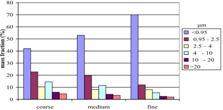
particulate matter. Any other substance can be computed if specific substance-related properties, such as molecular weight, surface resistance for dry deposition, scavenging ratio for wet deposition are provided. For particulate matter, six size classes are used and several particle size distributions, each with its own deposition characteristics, are available. Below, the standard particle size distributions 'coarse', 'medium' and 'fine' are shown (Figure 1). It is also
possible to specify a user defined particle size distribution.
0 10 20 30 40 50 60 70 80
coarse medium fine
mass fra ction (%) <0.95 0.95 - 2.5 2.5 – 4 4 - 10 10 - 20 >20 μm
Page 16 of 53
Meteo
Meteorological data have to be supplied as hourly data and are supposed to be representative for the model domain. OPS-ST uses the following meteo
parameters as input: wind speed, wind direction, temperature, pressure, relative humidity, global radiation, cloud cover and precipitation. A pre-processor is available that converts hourly data of KNMI stations in the Netherlands to meteo data for six regions in the Netherlands.
Emissions
The standard emission file of OPS specifies the location and yearly averaged emission for each emission source. If needed, the heat content of the source can be specified, in order to compute the plume rise. Depending on the specification in the emission file, emission characteristics such as daily and monthly profile are used in the OPS-ST model. For ammonia, OPS-ST divides emissions into animal housing and manure application emissions, each with their specific emission characteristics. If detailed hourly emission data is available, these can be specified in a special hourly emission file.
Validation
The capability of the model to simulate local dispersion has been tested against well-known datasets such as the Kincaid (Bowne and Londergan 1983) and Prairie grass datasets (Barad 1958). For larger scale transport of gases as SO2,
NOx and NH3, the model is successfully compared to results of the Dutch
National Air Quality Monitoring Network. Furthermore, the model has been subjected to several model intercomparison studies (e.g., Theobald et al. 2010) and has been used in studies on dispersion of ammonia (van Pul et al. 2008) and sea-salt (van Jaarsveld and Klimov 2011).
4
Calculations of Q fever dispersion with OPS
For the two cases Voerendaal and Helmond (Chapter 2), calculations of Q fever dispersion with the OPS model were carried out. We will first describe the set up of the cases and some sensitivity runs. Subsequently, the results of the
calculations for these cases will be presented. 4.1 Case 1: set-up
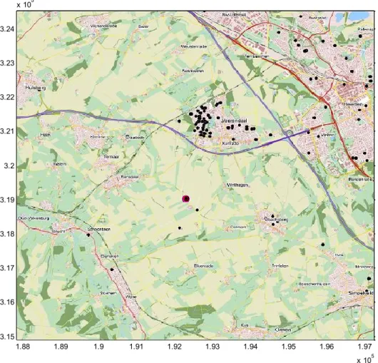
Case 1 is an outbreak of Q fever at Voerendaal in the Province of Limburg in 2009 (Figure 2). 1.88 1.89 1.9 1.91 1.92 1.93 1.94 1.95 1.96 1.97 x 10⁵ 3.15 3.16 3.17 3.18 3.19 3.2 3.21 3.22 3.23 3.24 x 10⁵
Figure 2: Map of modelled domain around Voerendaal. Red dot: farm. Black dots: human cases of Q fever reported in 2009.
Based on preliminary test runs (see appendix B.), the following default set-up was defined:
Q fever bacteria are treated as particles, with the standard OPS 'coarse' particle size distribution
single point source, emission height = 3 m
threshold wind velocity = 4 m/s. This means that in low wind conditions, bacteria are accumulated in the stable, in high wind conditions (velocity
Page 18 of 53
higher than threshold), all bacteria inside the stable are released in one hour.
dry deposition according to the dry deposition module DEPAC for particles
OPS meteorological region 6 (Limburg) roughness length = 0.20 m
receptor height = 1.5 m.
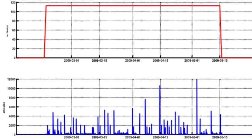
The effect of the threshold velocity is shown in Figure 3 and Figure 4 for
two different emission distributions. Since we do not yet know the actual amount of bacteria that is released, only relative concentrations (scaled between 0 and 1) will be used. This means that the unit for the y-axis in the following figures is not relevant. 2009-03-01 2009-03-15 2009-04-01 2009-04-15 2009-05-01 2009-05-15 0 20 40 60 80 100 120 em is si o n 2009-03-01 2009-03-15 2009-04-01 2009-04-15 2009-05-01 2009-05-15 0 2000 4000 6000 8000 10000 12000 vthreshold = 4 m/s em is si o n
Figure 3: Fictitious emission for Q fever simulations; upper panel shows
emission inside the stable, a uniform distribution in time during the period 2009-02-15 to 2009-05-15. The lower panel shows the emission that is released from the stable with a threshold wind velocity of 4 m/s. Arbitrary units.
2009-03-01 2009-03-15 2009-04-01 2009-04-15 2009-05-01 2009-05-15 0 20 40 60 80 100 120 em is si o n 2009-03-01 2009-03-15 2009-04-01 2009-04-15 2009-05-01 2009-05-15 0 2000 4000 6000 8000 10000 12000 vthreshold = 4 m/s em is si o n
Figure 4: Fictitious emission for Q fever simulations; upper panel shows
emission inside the stable, a skewed distribution in time with peak value at April
1st 2009. The lower panel shows the emission that is released from the stable
4.2 Case 1: sensitivity runs
A very limited sensitivity study was performed to show the sensitivity of OPS results on the threshold velocity, the particle size distribution and emission profile. Default settings were used and a uniform emission distribution, as in Figure 3.
An example of an input file for OPS is shown in appendix A. A list of all OPS runs in shown in appendix B.
OPS results are presented in Figure 5 as an average concentration over the period 2009-02-01 to 2009-05-31; for the sensitivity runs we used a grid
located around the farm with 50 x 50 receptors, 200 m grid resolution. Since the actual amount of Q fever bacteria emitted is yet unknown, concentrations here are presented as relative concentrations between 0 and 1 (concentrations for all runs are scaled with the same factor).
0 1e-005 0.0001 0.001 0.01 0.1 1 -5000 0 5000 -5000 -4000 -3000 -2000 -1000 0 1000 2000 3000 4000 5000
2009-05-31 12:00, test q-fever region 6, default settings OPS-ste/v 4.1, run 19 (2010-03-11 14:37) 0 1e-005 0.0001 0.001 0.01 0.1 1 -5000 0 5000 -5000 -4000 -3000 -2000 -1000 0 1000 2000 3000 4000 5000
2009-05-31 12:00, test q-fever region 6, default + v
threshold = 8 m/s OPS-ste/v 4.1, run 20 (2010-03-11 14:38) 0 1e-005 0.0001 0.001 0.01 0.1 1 -5000 0 5000 -5000 -4000 -3000 -2000 -1000 0 1000 2000 3000 4000 5000
2009-05-31 12:00, test q-fever region 6, default + vthreshold = 2 m/s OPS-ste/v 4.1, run 21 (2010-03-11 14:39) 0 1e-005 0.0001 0.001 0.01 0.1 1 -5000 0 5000 -5000 -4000 -3000 -2000 -1000 0 1000 2000 3000 4000 5000
2009-05-31 12:00, test q-fever region 6, default + vthreshold = 0 m/s OPS-ste/v 4.1, run 22 (2010-03-11 14:39)
Page 20 of 53 0 1e-005 0.0001 0.001 0.01 0.1 1 -5000 0 5000 -5000 -4000 -3000 -2000 -1000 0 1000 2000 3000 4000 5000
2009-05-31 12:00, test q-fever region 6, default + extra coarse particles OPS-ste/v 4.1, run 24 (2010-03-11 14:41) 0 1e-005 0.0001 0.001 0.01 0.1 1 -5000 0 5000 -5000 -4000 -3000 -2000 -1000 0 1000 2000 3000 4000 5000
2009-05-31 12:00, test q-fever region 6, default + uniform emission 1/2 Feb - 1/2 Mar OPS-ste/v 4.1, run 25 (2010-03-11 14:41)
Figure 5: OPS scaled concentrations (0-1), for runs 019, 020, 021, 022, 024, 025 (starting upper-left). Sensitivity on threshold velocity vt, particle size distribution and emission period.
19: vt = 4 m/s 20: vt = 8 m/s
21: vt = 2 m/s 22: vt = 0 m/s
24: vt = 4 m/s, extra coarse particles 25: emission in 1 month, vt = 4 m/s
From these figures we may conclude that the threshold velocity for emissions is a sensitive parameter in the modelling process.
We investigated the sensitivity of the model results on the emissions by using three types of emission profiles (Figure 6).
2009-02-01 2009-03-01 2009-04-01 2009-05-01 2009-06-01
2009 emission type A (uniform) emission type B (peak at Apr 1)
emission type C (peak at Apr 1, more spreading)
Figure 6: Three different emission types for emission inside the stable, with different distributions in time (peak value and spread in time). Arbitrary y-axis.
In order to be able to compare the OPS results to actual data on human Q fever cases, we processed the OPS concentrations as follows:
1. multiply the concentration with the number of inhabitants in each grid cell.
We assume here that the chance of becoming infected is linearly dependent on the concentration. However, since we do not know the actual amount of bacteria that is released, we have to scale:
2. Scale the (concentration x inhabitants) values such that the number of modelled cases inside the whole domain is equal to the number of reported cases.
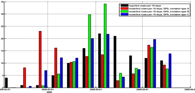
By doing so, we can compare the modelled cases that are infected per 10 days to the reported cases (Figure 7).
2009-02-010 2009-03-01 2009-04-01 2009-05-01 2009-06-01 5 10 15 20 25 30 35 2009
reported cases per 10 days
modelled cases per 10 days, OPS, emission type A modelled cases per 10 days, OPS, emission type B modelled cases per 10 days, OPS, emission type C
Figure 7: Number of human cases of Q fever in the modelled domain per 10 days for different emission types. Shown is the time of infection (assuming an incubation time for reported cases of 21 days). In black the number of reported cases, the other colours show modelled cases for the three different emission types from Figure 6.
In next sections of this report, we will use emission type C, since it matches best with the time distribution of the reported cases; the other types show large outliers compared to the reported number of cases.
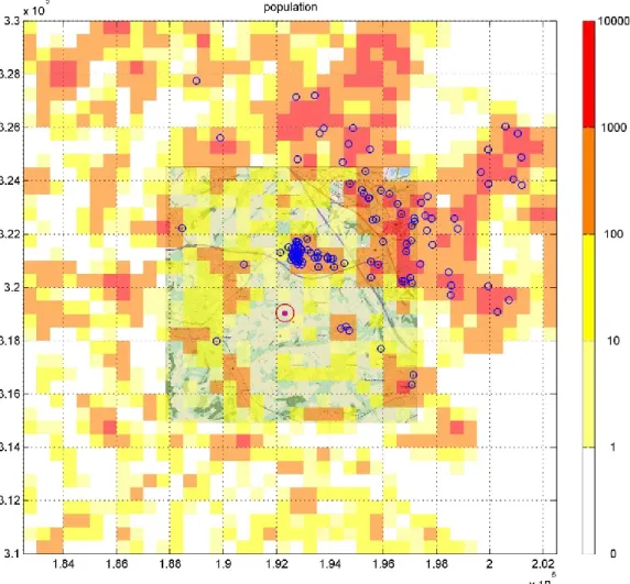
4.3 Case 1: Comparing OPS concentrations with reported Q fever cases In order to compare the OPS concentrations to the reported cases of Q fever around the farm at Voerendaal, new runs were performed with a grid based on a population density grid, which was available at a 500 m grid resolution (Figure 8).
Page 22 of 53
Figure 8: 20 x 20 km2 grid around the farm at Voerendaal with population
numbers. Blue circles: reported cases of Q fever infected during the test period 2009-02-01 to 2009-05-31 (assuming an incubation time of 21 days). Red circle: farm.
We used the default settings as before (threshold velocity for emission of 4 m/s) and emission type C. Results are presented as an average concentration over the period 2009-02-01 to 2009-05-31 (Figure 9).
Figure 9: 20 x 20 km2 grid around the farm at Voerendaal with OPS
concen-trations; emissions (type C) released for wind velocities > 4 m/s (run 038). Blue dots: reported cases of Q fever during the test period. Red circle: farm. Colours denote relative concentrations between 0 and 1.
Comparing OPS model results with reported Q fever cases will provide insight into the ability of OPS to model the dispersion of the Q fever bacteria. Since we want to evaluate the performance of the OPS model, we have set up two other simple models to compare with:
model 0: assume a uniform concentration over the whole domain
model 1: assume a concentration distribution ~ 1/r2, with r the distance to the
farm.
In order to obtain a measure for the distribution of human Q fever cases, we assumed that the number of cases per inhabitant in a grid cell is linearly dependent on the concentration in the grid cell and scaled the models such that the modelled number of cases in the whole domain was equal to the number of reported cases. The results (cases/inhabitant) can be shown as a grid (Figure
Page 24 of 53
10), but also in the form of scatter plots (Figure 11, x-axis: reported cases/inhabitant, y-axis: modelled cases/inhabitant).
0 0.0001 0.0002 0.0005 0.001 0.002 0.005 0.01 0.02 0.05 0.1 1.84 1.86 1.88 1.9 1.92 1.94 1.96 1.98 2 2.02 x 10⁵ 3.1 3.12 3.14 3.16 3.18 3.2 3.22 3.24 3.26 3.28 3.3x 10
5 model 0: cases per inhabitant
0 0.0001 0.0002 0.0005 0.001 0.002 0.005 0.01 0.02 0.05 0.1 1.84 1.86 1.88 1.9 1.92 1.94 1.96 1.98 2 2.02 x 10⁵ 3.1 3.12 3.14 3.16 3.18 3.2 3.22 3.24 3.26 3.28 3.3x 10
5 OPS: cases per inhabitant
Figure 10: 20 x 20 km2 grid around farm at Voerendaal with Q fever cases per
inhabitant; emissions (type C) released for wind velocities > 4 m/s (run 038). Top-left: reported cases; top-right: model 0 (uniform concentrations); bottom-left: model 1 (concentrations ~1/r2); bottom-right: OPS.
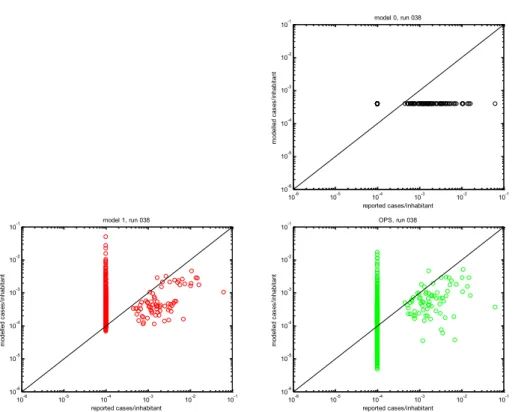
10-6 10-5 10-4 10-3 10-2 10-1 10-6 10-5 10-4 10-3 10-2 10-1 reported cases/inhabitant m od el le d ca se s/ in ha bi ta nt model 0, run 038 10-6 10-5 10-4 10-3 10-2 10-1 10-6 10-5 10-4 10-3 10-2 10-1 reported cases/inhabitant m od el le d ca se s/ in ha bi ta nt model 1, run 038 10-6 10-5 10-4 10-3 10-2 10-1 10-6 10-5 10-4 10-3 10-2 10-1 reported cases/inhabitant m od el le d ca se s/ in ha bi ta nt OPS, run 038
Figure 11: Scatter plot (log-log scale) for all grid cells in a 20 x 20 km2 grid
around the farm at Voerendaal with Q fever cases per inhabitant; emissions (type C) released for wind velocities > 4 m/s (run 038). Top-right: model 0 (uniform concentrations); left: model 1 (concentrations ~1/r2); bottom-right: OPS. Grid cells with no reported Q fever cases have been set to an
arbitrary low value (10-4), in order to show them in the plot.
From both Figure 10 and Figure 11, we may conclude that the OPS model performs better than model 0. Comparing OPS with model 1, the main difference is the cluster of grid cells which have no reported Q fever cases; for model 1 this cluster is in the range of [10-4 – 10-2] (mean value: 6.1 10-4)cases per
inhabitant, for OPS in the range of [10-6 10-2] (mean value 3.5 10-4) cases per
inhabitant.
In Figure 12, we sorted the incidence rates (number of cases per inhabitant) for model 1 and OPS, clustered them into three classes of equal length ('low risk', 'medium risk' and 'high risk') and plotted the reported incidence rates and human Q fever cases for these clusters of grid cells.
Page 26 of 53 model 1 OPS 0 0.2 0.4 0.6 0.8 1 1.2 x 10 -3 ca se s/i nh ab ita nt Voerendaal low risk medium risk high risk model 1 OPS 0 20 40 60 80 100 120 cases Voerendaal low risk medium risk high risk
Figure 12: Data clustered into three classes (low risk, medium risk, high risk) for Voerendaal, 2009. Upper panel: incidence rates (i.e., number of cases between 2009-02-01 and 2009-05-31 per inhabitant for each grid cell). Lower panel: number of human cases of Q fever.
From Figure 12, we see that OPS is slightly better in separating the low risk grid cells from other cells; the ratio of incidence rates of the high risk and the low risk classes are 11.7 for model 1 and 12.7 for OPS.
Another possible application of the OPS model data is to see what the average concentration profile in time is for a patient. A separate run was done (run 041) on the 20 x 20 km2 domain, where we used the location of the Q fever cases as
receptors for OPS. An average concentration profile was computed with respect to the date of onset of each case (Figure 13).
-130 -120 -110 -100 -90 -80 -70 -60 -50 -40 -30 -20 -10 Date-of-onset 0 0.1 0.2 0.3 0.4 0.5 0.6 0.7 0.8 0.9 1 days
Figure 13: Average concentration profile in time (3-day average). The averaging is over all cases (124 patients) in the modelled domain, taking the date of onset of each case as the reference time (blue line). Highest concentration before the date of onset is at 23 days before. The incubation time for Q fever is estimated to be 2-3 weeks (Parker et al. 2006).
Page 28 of 53
4.4 Case 2: set-up
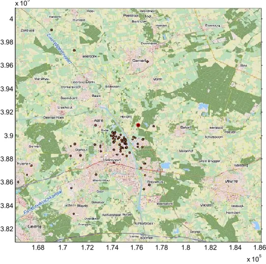
Case 2 is the outbreak of Q fever near Helmond in 2008 (Figure 14).
1.68 1.7 1.72 1.74 1.76 1.78 1.8 1.82 1.84 1.86 x 10⁵ 3.82 3.84 3.86 3.88 3.9 3.92 3.94 3.96 3.98 4 x 10⁵
Figure 14: Map of modelled domain around Helmond. Red dot: farm. Brown dots: human cases of Q fever reported in 2008.
The modelling set-up was more or less the same as before:
Q fever bacteria are treated as particles, with the standard OPS 'coarse' particle size distribution
single point source, emission height = 3 m threshold wind velocity 4 m/s
dry deposition according to the dry deposition module DEPAC for particles
OPS meteorological region 5 (Brabant) roughness length = 0.20 m
receptor height = 1.5 m. 4.5 Case 2: sensitivity runs
We did not repeat all the sensitivity runs of the previous case but tried several different types of emission distribution and compared the predicted number of cases per 10 days to the reported number of cases in the modelled domain. As before, modelling results were scaled such that the total number of modelled
cases was equal to the number of reported cases in the domain. A grid of 500 m resolution, with an area of 20 x 20 km2 around Helmond was used. Because a
uniform emission distribution does not fit the data well and the timing of the emission peak was not known, we assumed here the following three emission profiles (Figure 15) and computed the number of Q fever cases with OPS (Figure 16).
2008-04-01 2008-05-01 2008-06-01 2008-07-01 2008-08-01 2008-09-01 2008-10-01 emission type 1 (peak at Apr 15) emission type 2 (peak at May 1) emission type 3 (peak at May 15)
Figure 15: Three different emission types, with different distributions in time (peak value and spread in time). Arbitrary y-axis.
2008-04-010 2008-05-01 2008-06-01 2008-07-01 2008-08-01 2008-09-01 5 10 15 20 25 30 35 40 45 2008
reported cases per 10 days
modelled cases per 10 days, OPS, emission type 1 modelled cases per 10 days, OPS, emission type 2 modelled cases per 10 days, OPS, emission type 3
Figure 16: Number of human cases of Q fever in the modelled domain per 10 days for different emission types. Shown is the time of infection (assuming an incubation time for reported cases of 21 days). In black the number of reported cases, the other colours show modelled cases for three different emission types from Figure 15.
Emission type 2 seems to fit the reported cases best and will be used in the following analysis.
Page 30 of 53
4.6 Case 2: Comparing OPS concentrations with reported Q fever cases The location of the farm, the reported human Q fever cases and the number of inhabitants in each grid cell are shown in Figure 17.
Figure 17: 20 x 20 km2 grid around the farm at Helmond with population
numbers. Blue dots: reported cases of Q fever infected during 2008. Red circle: farm.
Average OPS concentrations during the test period 2008-04-01 to 2008-09-01 (emission type 2) are presented in Figure 18.
Figure 18: 20 x 20 km2 grid around the farm at Helmond with OPS
concentrations; emissions released for wind velocities > 4 m/s and emission type 2 (run 036). Blue dots: reported cases of Q fever during the test period. Red circle: farm. Colours denote relative concentrations between 0 and 1.
As before, we used two other models to compare the model results to the reported number of cases per inhabitant (Figure 19 and Figure 20).
Page 32 of 53 0 0.0001 0.0002 0.0005 0.001 0.002 0.005 0.01 0.02 0.05 0.1 1.66 1.68 1.7 1.72 1.74 1.76 1.78 1.8 1.82 1.84 1.86 x 10⁵ 3.82 3.84 3.86 3.88 3.9 3.92 3.94 3.96 3.98 4 x 10⁵ reported cases/inhabitant 0 0.0001 0.0002 0.0005 0.001 0.002 0.005 0.01 0.02 0.05 0.1 1.66 1.68 1.7 1.72 1.74 1.76 1.78 1.8 1.82 1.84 1.86 x 10⁵ 3.82 3.84 3.86 3.88 3.9 3.92 3.94 3.96 3.98 4
x 105 model 0: cases per inhabitant
0 0.0001 0.0002 0.0005 0.001 0.002 0.005 0.01 0.02 0.05 0.1 1.66 1.68 1.7 1.72 1.74 1.76 1.78 1.8 1.82 1.84 1.86 x 10⁵ 3.82 3.84 3.86 3.88 3.9 3.92 3.94 3.96 3.98 4
x 105 model 1: cases per inhabitant
0 0.0001 0.0002 0.0005 0.001 0.002 0.005 0.01 0.02 0.05 0.1 1.66 1.68 1.7 1.72 1.74 1.76 1.78 1.8 1.82 1.84 1.86 x 10⁵ 3.82 3.84 3.86 3.88 3.9 3.92 3.94 3.96 3.98 4
x 105 OPS: cases per inhabitant
Figure 19: 20 x 20 km2 grid around the farm at Helmond with Q fever cases per
inhabitant; emissions released for wind velocities > 4 m/s and emission type 2 (run 036). Top-left: reported cases; top-right: model 0 (uniform
concentrations); bottom-left: model 1 (concentrations ~1/r2); bottom-right: OPS.
10-4 10-3 10-2 10-1 100 10-4 10-3 10-2 10-1 100 reported cases/inhabitant m od el le d ca se s/ in ha bi ta nt model 0, run 036 10-4 10-3 10-2 10-1 100 10-4 10-3 10-2 10-1 100 reported cases/inhabitant m od el le d ca se s/ in ha bi ta nt model 1, run 036 10-4 10-3 10-2 10-1 100 10-4 10-3 10-2 10-1 100 reported cases/inhabitant m od el le d ca se s/ in ha bi ta nt OPS, run 036
Figure 20: Scatter plot (log-log scale) for all grid cells in a 20 x 20 km2 grid
around the farm at Helmond with Q fever cases per inhabitant; emissions released for wind velocities > 4 m/s and emission type 2 (run 036). Top-right: model 0 (uniform concentrations); bottom-left: model 1 (concentrations ~1/r2); bottom-right: OPS. Grid cells with no reported Q fever cases have been set to an
arbitrary low value (10-4), in order to show them in the plot.
The cluster of grid cells which have no reported Q fever cases has a mean value for model 1 of 5.0 10-4 cases per inhabitant, for OPS 4.1 10-4 cases per
inhabitant.
In Figure 21, we sorted the incidence rates (number of cases per inhabitant) for model 1 and OPS, clustered them into three classes of equal length ('low risk', 'medium risk' and 'high risk') and plotted the reported incidence rates and human Q fever cases for these clusters of grid cells.
Page 34 of 53 model 1 OPS 0 1 2 3 4 5 6 7 8 x 10 -4 ca se s/i nh ab ita nt Helmond low risk medium risk high risk model 1 OPS 0 10 20 30 40 50 60 70 80 cases Helmond low risk medium risk high risk
Figure 21: Data clustered into three classes (low risk, medium risk, high risk) for Helmond, 2008. Upper panel: incidence rates (i.e., number of cases between 2009-02-01 and 2009-05-31 per inhabitant for each grid cell). Lower panel: number of human cases of Q fever.
From Figure 21, we see that OPS is much better in separating the low risk grid cells from other cells; the ratio of incidence rates of the high risk and the low risk classes are 5.8 for model 1 and 15.5 for OPS.
The average concentration profile in time for a patient is shown in Figure 22. -60 -50 -40 -30 -20 -10 Date-of-onset 0 0.1 0.2 0.3 0.4 0.5 0.6 0.7 0.8 0.9 1 days
Figure 22: Average concentration profile in time (3-day average). The averaging is over all cases (85 patients), taking the date of onset of each case as the reference time (blue line). Highest concentration before the date of onset is at 23 days before (as in case 1). The incubation time for Q fever is estimated to be 2-3 weeks (Parker et al. 2006).
This average concentration profile shows a peak at 23 days before the date of onset, which corresponds well with the expected incubation time of 2-3 weeks. Of course, one has to take into account that emissions have been tuned on the total number of cases per 10 days in the whole domain, but the dose
experienced by each patient may vary considerably, depending on the direction between farm and patient's address and the wind direction, as can be seen in Figure 23.
Page 36 of 53
Figure 23: Daily film frames of Q fever outbreak near Helmond during May 10 – 21, 2008. The colours show the 3-day running averages of relative
concentrations (0-1) computed by OPS, the black dots show reported Q fever cases that are infected on the current day (±1 day) assuming a 23-day incubation time.
Page 38 of 53
5
Discussion and conclusions
The OPS model is able to simulate the general behaviour of airborne Coxiella
burnetii dispersion. The distribution in space matches the general patterns of
reported human Q fever cases. The distribution in time (number of cases per ten days) can be matched reasonably well by assuming a simple emission profile.
The average concentration profile in time shows a peak in concentration some 23 days before the date of onset of Q fever. This corresponds well with the incubation time of Q fever, which is usually 2-3 weeks with 4 days and 6 weeks representing the extremes (Parker et al. 2006).
The main difficulty in simulating Q fever dispersion is the lack of emission data. We tried to circumvent the problem of timing of the release of Q fever bacteria by postulating several emission profiles. The resulting temporal behaviour of modelled Q fever cases was evaluated against reported cases. From that, the most appropriate emission profile from a pre-defined set of candidates was chosen. The problem of not knowing the amount of bacteria released was circumvented by a scaling procedure, such that the total amount of modelled cases in the modelled domain was the same as the number of reported cases. One could argue that these procedures involve a-priori information that is not known normally.
In the two cases studied here, the main parameters that describe the
distribution of human Q fever cases are the population density and distance to the farm. We compared OPS results with the results of two simple models: model 0 (assuming a uniform concentration distribution) and model 1
(concentration distribution ~ 1/r2, with r the distance to the farm). Comparing
low, medium and high risk areas, model 1 and OPS show that the risk of Q fever highly depends on the distance to the source. OPS adds extra information (wind direction and other dispersion related parameters) and computes lower average incidence rates in 'low risk' grid cells than the other models (see Figure 12 and Figure 21). Furthermore, OPS provides temporal information, which is
completely missing in the other models.
Another difficulty in the simulation process lies in the fact that this study is based on the assumption that people receive their dose of Q fever bacteria whilst being 24/7 at home. More information on human activities during the day could improve results.
In this study, no detailed information on the soil and vegetation conditions was taken into account. These conditions play an important role in the amount of aerosol that is deposited from the air (Hunink et al. 2010). It is known that aerosol may resuspend again, in which surface characteristics such as wetness are an important parameter.
To reduce the uncertainty in the calculation, more information on the following items should become available:
time and amount of bacteria released at a farm influence of external factors on the emission:
o wind velocity; does a threshold velocity exist below which no emission takes place?
o length of the dry period before emission o wind gusts
o wind direction with respect to geometry of stable o open stable – mechanically ventilated stable dispersion
o particle size distribution o deposition parameters exposure
o human activities o dose-response relation re-emission
o linkage with soil dust
6
Acknowledgements
We thank the Municipal Health Services of Zuid Limburg and Brabant Zuidoost for providing location data of human Q fever cases.
This study was done as a pilot project to prepare for a larger study under the RIVM/SOR project ‘Environmental risk factors for Q fever’, project number S/210106/01/RQ.
7
References
Barad ML, editor (1958) Project Prairie Grass, a field program in diffusion. Volume 1, Geophysics Research Paper no. 59. Geophysics Research Directorate, Air Force Cambridge Research Center, Cambridge MA, USA.
Benenson AS, Tigertt WD. Studies on Q fever in man. Trans Assoc Am Physicians. 1956; 69:98-104
Bowne NE and Londergan RJ (1983) Overview, results and conclusions for EPRI Plume Model Validation and Development Project: Plains site, EPRI, Palo Alto, California 94304.
van der Hoek W, Dijkstra F, Schimmer B, Schneeberger PM, Vellema P, Wijkmans C, ter Schegget R, Hackert V, van Duynhoven Y. Q fever in the Netherlands: An update on the epidemiology and control measures. Euro Surveill. 2010;15(12):pii=19520. Available online:
http://www.eurosurveillance.org/ViewArticle.aspx?ArticleId=19520
Hunink JE, Veenstra T, van der Hoek W, Droogers P (2010). Q fever
transmission to humans and local environmental conditions. Report FutureWater 90, January 2010. http://www.rivm.nl/cib/binaries/Q
fever%20transmission_tcm92-66769.pdf
van Jaarsveld JA 2004. ‘The Operational Priority Substances model’. Description and validation of OPS-Pro 4.1. RIVM/MNP report 500045001/2004. RIVM, P.O. Box 1, 3720 BA Bilthoven
van Jaarsveld JA and Klimov D. 2011. Modelling the impact of sea-salt particles on the exceedances of daily PM10 air quality standards in the Netherlands. To appear in Int. J. Environment and Pollution.
Parker NR, Barralet JH, Bell AM. Q fever. Lancet. 2006 Feb 25;367(9511):679-88.
van Pul W.A.J., van Jaarsveld J.A., Vellinga O.S., van den Broek M, Smits M.C.J. The VELD experiment: An evaluation of the ammonia emissions and
concentrations in an agricultural area. Atmospheric Environment 2008 11;42(34):8086-95.
Roest HI, Tilburg JJ, van der Hoek W, Vellema P, van Zijderveld FG, Klaassen CH, et al. The Q fever epidemic in the Netherlands: history, onset, response and reflection. Epidemiol Infect. 2010 Oct 5:1-12.
Schimmer B, Ter Schegget R, Wegdam M, Zuchner L, de Bruin A, Schneeberger PM, Veenstra T, Vellema P, van der Hoek W. The use of a geographic information system to identify a dairy goat farm as the most likely source of an urban Q fever outbreak. BMC Infect Dis. 2010 Mar 16;10(1):69.
Tamrakar SB, Haluska A, Haas CN and Bartrand TA (2011), Dose-Response Model of Coxiella burnetii (Q Fever). Risk Analysis, 31: 120–128.
Page 44 of 53
Theobald MR, Løfstrøm P, Andersen HV, Pedersen P, Walker J, Vallejo A. and Sutton M. An intercomparison of models used to simulate the atmospheric dispersion of agricultural ammonia emissions. 13th Conference on harmonisation within Atmospheric Dispersion Modelling for Regulatory Purposes, 1-4 June 2010, Paris , France
Appendix A. OPS input file
Default .ops input file:
settings.ops
############################################################################ ###
Operational Atmospheric Transport Model for Priority Substances - Short Term Edition -
MODEL - SETTINGS FILE
############################################################################ ###
IMPORTANT: Do NOT change the first line above and the lay-out of sections "RUN OPTIONS" and "DIRECTORY PATHS" in this file, otherwise OPS-Ste might not work (properly)!
RUN OPTIONS ---
1 | General Settings
| - automatically quit after run (+) __________ : n | (for mutiple run-sessions with .BAT-file) |
| if 'no' auto-quit then:
| - detailed information to screen (+) ______ : y |
| - name simulation run _______________________ : q019 |
2 | Select Component ____________________________ : 4
| (1= SO2, 2= NO2, 3= NH3, 4= Particles, 5= User-Defined($)) |
| if "Particles" or "User-Defined" then:
| - select particle-size distribution _________ : 1
| (0= none, 1= coarse, 2= medium, 3= fine, 4= user-defined) |
| if "User-Defined" then:
| - name particle-size distribution-file (.psd): USER_DEFINED |
3 | Area Characteristics
| - name meteorological file ___________________ : 2009\rg6mbk09 | - surface-resistance (Rc) data ______________ : 1
| (0= Constant; 1= Variable (DEPAC-module)) |
| if 0 then:
Page 46 of 53
|
| - roughness length data ($) _________________ : 0 | (0= Single Value, 1= Roughness-Length Map) |
| if 0 then ($):
| - overall roughness length [m] ____________ : 0.20 | if 1 then ($):
| - name file roughness-length map (.rgh) ___ : ROUGHNESSFILENAME ! - Other meteo parameters:
| - altitude wind obs.________________________ : 10. ! - z0 used for meteo data ___________________ : 0.03 | (0= overall z0 is used)___________________ |
4 | Time Period & Averaging
| - start run (yy mm dd hh) ___________________ : 09 01 01 01 | - end run (yy mm dd hh) ___________________ : 09 12 31 24 | - type of averaging _________________________ : 4
| (0= Total Period, 1= Year, 2= Month, 3= Day, 4= Hour) |
5 | Source Configuration ________________________ : 1 | (0= constant, 1= variable [hourly])
|
| if 0 then:
| - name constant source file (.src) __________ : none | - select source category (0000 = all) ______ : 0000 | - select country area (0000 = all) _________ : 0000 | if 1 then:
| - name hourly emission file (.ems) ________ : testq_2009_uni_1 |
6 | Receptor Configuration ______________________ : 0 | (0= Model Grid, 1= Specific Receptor(s))
|
| if 0 then:
| - receptor-grid height [m] (#) _____________ : 1.5
| - grid centre co-ordinates [m] (*) _________ : 0.0 0.0 | - number of grid elements [x & y dir.] (#) __ : 50 50
| - grid resolution [m] (#) __________________ : 200 | if 1 then:
| - name of receptor file (.rcp) ______________ : _ |
7 | Also percentiles? (+) ______________________ : n |
| if 1 then:
| - percentile value (001 - 100) _____________ : 098 | - incl. background concentration (+) _______ : y |
8 | Also dry deposition? (+) ___________________ : y NOTES:
(+) Choose: n = no; y = yes (**) Valid range: 0 - 10000
(*) Dutch co-ordinate system called "Amersfoorste co-ordinate system". For
the Netherlands ranges are: 013000.0 <= x <= 278000.0 and 306000.0 <= y <= 620000.0 .
(#) Valid range: 000 - 999 ($) Not yet available !!!
--- DIRECTORY PATHS ---
INPUT PATHS:
annual source-emission (.src) __ : D:\proj\ops\OPS-KT\input\src\ hourly emission (.ems) _________ : ..\data\emis\
meteorlogical data ______________ : D:\proj\ops\OPS-KT\input\met\ partical size-distribution (.psd) : D:\proj\ops\OPS-KT\input\psd\ receptor(s) (.rcp) _____________ : D:\proj\ops\OPS-KT\input\rcp\ map of roughness lengths (.rgh) : D:\proj\ops\OPS-KT\input\rgh\ OUTPUT PATH:
output _________________________ : ..\data\output\q019\
NOTE: If directory path is kept open, OPS-STe will look for\save files into same folder as where the model has been put.
---- DESCRIPTION SIMULATION RUN ---
...
############################################################################ ###
Copyright 1992-2002 RIVM, 2003-2004 MNP-RIVM (Bilthoven, The Netherlands)
Appendix B. OPS runs
Preliminary test runs
Preliminary test runs were done to check whether OPS performs as expected and to check that everything works. Emissions in these runs are presented in Figure 24.
2008-12-010 2009-02-01 2009-04-01 2009-06-01 2009-08-01 2009-10-01 2009-12-01 2010-02-01 1
2
3 simple emission model Q-fever [fictional data] (total emission 1 animal = scaled to 100)
em is si o n d if fe re n t an im al g ro u p s 2009 10 100 20 2008-12-010 2009-02-01 2009-04-01 2009-06-01 2009-08-01 2009-10-01 2009-12-01 2010-02-01 100 200 300 2009 su m m ed e m is si o n o f 13 0 an im al s 2008-12-010 2009-02-01 2009-04-01 2009-06-01 2009-08-01 2009-10-01 2009-12-01 2010-02-01 100 200 300 v threshold = 0 m/s 2009 su m m ed e m is si o n o f 13 0 an im al s
Figure 24: Fictive emission for preliminary Q fever simulations; upper panel three lognormal distributions in time, for three groups of animals with 10, 100 and 20 animals. Second panel: summed emission. Third panel: emission without a threshold wind velocity. Fourth panel: emission with a threshold wind velocity of 2 m/s. Fifth panel: emission with a threshold wind velocity of 4 m/s.
Page 50 of 53
Test runs for non-reactive gas, region 6 (Voerendaal)
Test runs with emissions as area source d = 25 m, h = 0 m.
run emission file
remarks
001 testq_2005.ems
test-emission 2005, no threshold
velocity
002 testq_2008.ems
test-emission 2008, no threshold
velocity
003 testq_2009.ems
test-emission 2009, no threshold
velocity
004 testq_2009_v0.ems
test-emission 2009, threshold
velocity for emission = 0 m/s
005 testq_2009_v2.ems
test-emission 2009, threshold
velocity for emission = 2 m/s
006 testq_2009_v4.ems
test-emission 2009, threshold
velocity for emission = 4 m/s
007 testq_2009_shift30.ems
test-emission 2009, source
location shifted to (30,30) no
important differences in plume
008 testq_2009_shift50.ems
test-emission 2009, source
location shifted to (50,50)
=> OPS crashes, dsx = 0; divide
by 0
Test runs with emissions as point source d = 0 m, h = 0 m, threshold
velocity = 4 m/s
009 testq_2009_p_shift0.ems
test-emission 2009, point source
location shifted to (0,0)
010 testq_2009_p_shift30.ems
test-emission 2009, point source
location shifted to (30,30)
011 testq_2009_p_shift50.ems
test-emission 2009, point source
location shifted to (50,50)
no important differences in
plume; extremely high values near
farm (receptor at source location)
Test runs with emissions as point source d = 0 m, h = 3 m, threshold
velocity = 4 m/s, source at (0,0)
012
testq_2009_p_shift0_h3.ems
test-emission 2009, h = 3 m
Test runs for particles, region 6 (Voerendaal)
Test runs with emissions as point source d = 0 m, h = 0 m, threshold
velocity = 4 m/s
run emission file
remarks
013
testq_2009_p_shift0_h3_psd3.ems
test-emission 2009,
'coarse' particles, source
at (0,0), longer
simulation period
(2009-06-01)
015
testq_2009_p_shift0_h3_psd3.ems
test-emission 2009,
'extra coarse' particles,
source at (0,0); user
defined psd
../data/psd/qfever1.psd
016a testq_2009_r6_p_shift0_h3_psd3.ems test-emission 2009,
'coarse' particles, source
at (0,0), emission/1000.
concentration = 0 !
016b testq_2009_r6_p_shift0_h3_psd3.ems test-emission 2009,
'coarse' particles, source
at (0,0), emission/10.
017
testq_2009_r6_p_shift0_h3_psd3.ems test-emission 2009,
'coarse' particles, source
at (0,0), emission,
receptor height = 1.5 m
018
testq_2009_r6_p_shift0_h3_psd3.ems test-emission 2009,
'coarse' particles, source
at (0,0), emission,
receptor height = 1.5 m,
grid resolution = 200 m.
Test runs for particles, region 3
Test runs with emissions as point source d = 0 m, h = 0 m, threshold
velocity = 4 m/s
run emission file
remarks
014 testq_2009_r3_p_shift0_h3_psd3.ems test-emission 2009,
'coarse' particles, source
at (0,0)
Test runs, farm at grid centre (0,0)
Test runs for particles, region 6 (Voerendaal)
Test runs with emissions as point source d = 0 m, h = 3 m, threshold
velocity = 4 m/s
grid resolution 200 m
run
emission file
remarks
019
testq_2009_uni_1.ems
default run
020
testq_2009_uni_2.ems
default + v_threshold = 8 m/s
plume only in certain directions
021
testq_2009_uni_3.ems
default + v_threshold = 2 m/s
plume spread over larger area,
concentrations higher
022
testq_2009_uni_4.ems
default + v_threshold = 0 m/s
more spread, concentrations
even higher
023
testq_2009_log_1.ems
default + emission log-normal
distribution in time
differences with default run 019
marginal; 019 somewhat larger
plume (more emission during
plot-period)
024
testq_2009_uni_1.ems
default + extra coarse particles
(4-10 µm: 20%, 10-20 µm: 60%,
> 20 µm: 20%).
plume somewhat smaller,
differences small with run 019.
025
testq_2009_uni_5.ems
default + uniform emission during
Page 52 of 53
2009-02-15 – 2009-03-15. Note
that the total emission is the same
as before, only the release is in a
shorter time span (1 month
instead of 3 months).
more concentrated plume in
some directions; no partial plumes
in other directions.
026
testq_2009_uni_1.ems
default + receptors = Q fever
cases near Voerendaal
027
testq_2009_uni_1.ems
default + grid resolution of 500 m.
Test runs, RDM coordinates
Test runs for particles, region 6 (Voerendaal)
Test runs with emissions as point source d = 0 m, h = 3 m, threshold
velocity = 4 m/s
Amersfoort-coordinates (RDM); grid coincides with population grid; grid
resolution = 500 m.
028
testq_2009_uni_ac_1.ems
default; grid 10x10 km
2
;
v_threshold = 4 m/s
029
testq_2009_uni_ac_1.ems
default; grid 20x20 km
2;
v_threshold = 4 m/s
030
testq_2009_uni_ac_2.ems
default; grid 20x20 km
2
;
v_threshold = 8 m/s
031
testq_2009_uni_ac_3.ems
default; grid 20x20 km
2
;
v_threshold = 2 m/s
032
testq_2009_uni_ac_4.ems
default; grid 20x20 km
2
;
v_threshold = 0 m/s
033
testq_2009_uni_ac_1.ems
default; receptors =
cases_voerendaal; v_threshold = 4
m/s;
037
testq_2009_vdaal_log_1
default; grid 20x20 km
2;
v_threshold = 4 m/s; emission type
B (t1=32; t2=92; =0.3)
038
testq_2009_vdaal_log_2
default; grid 20x20 km
2;
v_threshold = 4 m/s; emission type
C (t1=32; t2=92; =0.5)
039
testq_2009_vdaal_log_2
default; receptors =
cases_voerendaal; v_threshold = 4
m/s; emission type C (t1=32;
t2=92; =0.5)
041
testq_2009_vdaal_log_2
default; receptors =
cases_voerendaal2; v_threshold =
4 m/s; emission type C (t1=32;
t2=92; =0.5)
Test runs for particles, region 5 (Helmond)
Test runs with emissions as point source d = 0 m, h = 3 m, threshold
velocity = 4 m/s
Amersfoort-coordinates (RDM); grid coincides with population grid; grid
resolution = 500 m.
034
testq_2008_log_bakel_1.ems
default; grid 20x20 km
2
;
v_threshold = 4 m/s; emission
type 1 (t1=92; t2=106; =1).
035
testq_2008_bakel_log_2.ems
default; grid 20x20 km
2
;
v_threshold = 4 m/s; emission
type 3 (t1=30; t2=136;
=0.15).
036
testq_2008_bakel_log_3.ems
default; grid 20x20 km
2
;
v_threshold = 4 m/s; emission
type 2 (t1=92; t2=121; =0.5).
040
testq_2008_bakel_log_3.ems default; grid 20x20 km
2;
v_threshold = 4 m/s; emission
type 2 (t1=92; t2=121; =0.5).
Receptors = patients.
R.M. ter Schegget | V. Hackert |
W. van der Hoek
National Insitute for Public Health and the Environment
P.O. Box 1 | 3720 BA Bilthoven www.rivm.com