A Green Development Mechanism

(1)

Netherlands Environmental Assessment Agency, December 2009

Policy Studies

Is a ’Green Development Mechanism’ a useful policy instrument for

safe-guarding biodiversity?

That was the question of the Ministry of Housing, Spatial Planning and the Environment (VROM). This ‘Green Development Mechanism’ concept is an analogy of the Clean Development Mechanism under the Climate Convention. The concept implies that man should compensate biodiversity loss by the conservation of a similar amount of biodiversity elsewhere. Implemented at the global level, this would eventually result in the protection of 50% of the global biodiversity. Land ‘use’ for nature would be in direct competition with land use for agriculture and other forms of economic development. Nature would get a market price.

Key questions are whether there is sufficient biodiversity available to compensate losses, now and in the future, and where this biodiversity is located?

We concluded that compensation on the global scale is possible, but has limited effect on the average global biodiversity. Compensation within regions or within biomes does have significant effect on overall global biodiversity, although various biomes and regions already have serious compensation ‘deficits’. Compensation on smaller scales will not improve this result, but would provide a better representativeness of world’s biodiversity.

A Green

Development

Mechanism

(2)

(3)

A Green Development Mechanism

Biodiversity compensation on a

global, regional and biome scale

(4)

A Green Development Mechanism

Corresponding Author: M. Bakkenes; michel.bakkenes@pbl.nl

Parts of this publication may be reproduced, providing the source is stated, in the form: Netherlands Environmental Assessment Agency: Title of the report, year of publication. This publication can be downloaded from our website: www.pbl.nl/en. A hard copy may be ordered from: reports@pbl.nl, citing the PBL publication number.

The Netherlands Environmental Assessment Agency (PBL) is the national institute for strategic policy analysis in the field of environment, nature and spatial planning. We contribute to improving the quality of political and administrative decision-making by conducting outlook studies, analyses and evaluations in which an integrated approach is considered paramount. Policy relevance is the prime concern in all our studies. We conduct solicited and unsolicited research that is both independent and always scientifically sound.

Office Bilthoven PO Box 303 3720 AH Bilthoven The Netherlands Telephone: +31 (0) 30 274 274 5 Fax: +31 (0) 30 274 44 79 Office The Hague PO Box 30314 2500 GH The Hague The Netherlands

Telephone: +31 (0) 70 328 8700 Fax: +31 (0) 70 328 8799

(5)

Rapport in het kort 5 Biodiversiteitverlies compenseren op wereld, regio en

ecosysteem schaal. Een biodiversiteit compensatie mechanisme.

De groei van de wereldbevolking en -economie in de komende decennia leidt tot een aanhoudend verlies van biodiversiteit, ondanks de mondiale afspraak dit verlies af te remmen of te stoppen. Het behoud van biodiversiteit wordt als een voorwaarde gezien voor welvarende samenlevingen in de toekomst. Het Ministerie van VROM verkent daarom nieuwe beleidsinstrumenten. Eén daarvan is het zogenaamde ‘biodiversiteit compensatie mechanisme’, naar analogie van het Clean Development Mechanism in het klimaatbeleid. Uitgangspunt hierbij is dat elke door mensen vernietigde hoeveelheid biodiversiteit gecompenseerd wordt door een zelfde hoeveelheid beschermde hoeveelheid biodiversiteit elders. Dit leidt uiteindelijk tot een 50%-50% verdeling van de aarde tussen mens en overige levensvormen. Dit rapport bekijkt of er voldoende biodiversiteit resteert om te kunnen compenseren, in 2000 en 2050. Het blijkt dat compensatie steeds moeilijker wordt naarmate men deze strikter toepast. Op wereldschaal is er voldoende ruimte als men verlies van tropisch regenwoud kan compenseren met toendra. Maar compenseren binnen dezelfde regio of binnen hetzelfde ecosysteem wordt moeilijker. Voor sommige ecosystemen resteert nu al onvoldoende ruimte. In andere gevallen is de groeiende behoefte aan ruimte voor voedsel- en houtproductie een belemmering. Het is precies deze krapte die de prikkel moet geven tot intensivering van het huidige landgebruik, in plaats van het omzetten van meer natuur: geen expansie maar intensiveren. Het rapport beoogt een eerste beeld te geven van de fysieke mogelijkheden en beperkingen van dit beleidsinstrument aan beleidsmakers op dit terrein, zowel nationaal als internationaal. Het geeft geen analyse van de socio-economische, culturele en institutionele aspecten.

Trefwoorden / Keywords:

Biodiversity, Compensation, Green Development Mechanism, Offset, global, regional, biome

(6)

(7)

Rapport in het kort 7

This report is a first analysis of a ‘Green Development Mechanism’ concept as a novel policy instrument. The Dutch Ministry of Housing, Spatial Planning and the Environment (VROM) developed visions on this concept in 2008 as an analogy of the Clean Development Mechanism under the Climate Convention. The concept implies that man should compensate biodiversity loss in one location, by conserving a similar amount of biodiversity elsewhere. Implemented at the global level, this would eventually result in the protection of 50% of the global biodiversity. Land ‘use’ for nature would be in direct competition with land use for agriculture and other forms of economic development. Nature would get a market price.

The Ministry of VROM requested PBL to explore the

feasibility of this instrument. Key questions are: i) Is sufficient biodiversity available to compensate losses, now and in the future?, and ii) Where is this biodiversity located? The practicability and cost of this policy instrument, and socio-economic and cultural aspects are not part of this study. Methodology

We used the IMAGE/GLOBIO model for our calculations. Results are presented for two indicators of biodiversity, derived from the Convention on Biological Diversity: i) natural area; and ii) mean species abundance (MSA).

We calculated the possibility of biodiversity compensation on a: i) global scale, ii) regional scale, iii) biome scale, and iv) per regional biome, over the time period from 2000 to 2050, in a developing world, according to the OECD Baseline scenario. As an alternative scenario, we superimposed a 50% compensation scenario (biodiversity in protected areas) on the world, disregarding biodiversity deficits from other land uses. A 50% variant with a priority of protecting the most remote and highest quality natural areas, and a 50% variant with the priority of protecting the most threatened areas close to the agricultural areas in 2000. Subsequently, we analysed whether sufficient agricultural land and forestry would remain to cope with food and timber demand.

Results

In the Baseline scenario, by 2050, about 40% of all global land areas will be used by mankind. This is 47% of all productive areas – thus, excluding ice, tundra and desert. Compensation within smaller spatial units, regions, biomes or region-biome combinations, will lead to deficits. To date, central Europe,

the Ukraine region, the Kazakhstan region, and the Indian region, already lack sufficient biodiversity to compensate. This will become worse in the future. In general, the smaller the spatial scale of compensation and the later over time the higher the deficits. If only largely intact ecosystems (>80% quality) are judged suitable for compensation, the deficits can increase by up to 80% or more. Consequently, for several regions in the 50% compensation scenario, not all human demand for food, wood and other commodities, will be met, by 2050. However, this deficit may be solved by inter-regional trade and – as is the purpose of the Green Development Mechanism - by increasing production efficiency. Both could not be analysed within the means of this project.

Conclusion

Compensation on the global scale is possible, but has limited effect on the average global biodiversity, in terms of mean species abundance (MSA). Though Compensation within regions or biomes will have significant effect on overall global biodiversity. Compensation on smaller scales will not improve this result, but would provide a better representativeness. Fifty percent compensation is not always feasible, given the current land use and future needs, and would result in deficits for meeting human demands by 2050. However, these deficits could initiate increasing production efficiency, being the very reason of this policy instrument

(10)

(11)

Introduction 11 The loss of biodiversity of the last decades is expected to

continue into the coming decades (MEA, 2005; CBD/MNP, 2007; OECD, 2008; PBL, 2008). The main drivers of this loss, globally, are a growing population and economy resulting in a growing production and consumption. In turn, this will result in an increased loss in natural land and growing pressure from, among other things, climate change, pollution, fragmentation, and over-exploitation. European countries have set the target of halting biodiversity loss in Europe by 2010. Policymakers conclude that this target will not be achieved (LNV, 2008; EC, 2009). Policy options in the second Global Biodiversity Outlook (CBD/MNP, 2007) showed no sufficient solution to solve this.

One option for halting or reducing the rate of biodiversity loss is by increasing agricultural and forestry productivity. This could reduce two of the major causes: the conversion and overexploitation of natural habitats. Therefore, the Dutch Ministry of Housing, Spatial Planning and the Environment (VROM) developed visions on a novel policy instrument, a ‘Green Development Mechanism (GDM)’ concept, analogous to the Clean Development Mechanism under the UN Climate Convention. The concept as explored in this report is about compensating biodiversity loss by the conservation of a similar amount of biodiversity elsewhere. Implemented on a global level, this would eventually result in the protection of 50% of global biodiversity.

The Ministry of VROM requested the PBL to explore the feasibility of this policy instrument. Key questions were: i) is sufficient biodiversity available to compensate losses, now and in the future, and ii) where is this biodiversity located? This report is a first analysis of one concept of this novel policy instrument. Calculations were made with the IMAGE/ GLOBIO model, and results from the scenario calculations from the OECD Environmental Outlook to 2030 (OECD, 2008) were input for this analysis.

This analysis is not about which biodiversity would qualify to be protected or how to protect it, how people should be compensated and by whom, what the cost would be and how this could be organised1. Neither has this report worked out

the socio-economic and cultural aspects.

1 An elaboration on these issues can be found in Blom et al.,2008,

Chapter 1 describes the GDM concept as tentatively defined by the Ministry of VROM, and Chapter 2 describes the methodology we applied. Chapter 3 gives the results from the analyses, and Chapter 4 and 5 contain the conclusions and discussions. Tables that are related to Chapter 3, but not included in the chapter, can be found in Appendix I.

(12)

(13)

The Green Development Mechanism concept 13 The Dutch Ministry of Housing, Spatial Planning and the

Environment (VROM) developed the idea of a Green Development Mechanism (GDM), in 2008, as an analogy of the Clean Development Mechanism (CDM) under the United Nation’s Climate Convention. The GDM concept developed in this report starts from the assumption of the obligation to compensate biodiversity loss by the conservation of a similar amount of biodiversity elsewhere. Implemented on a global level, this would eventually result in the protection of 50% of global biodiversity. This ambitious level of protection would create direct competition between nature and agricultural land use, as well as other forms of economic development. As a means of compensation nature gets a market price, similar to CO2 emission rights. The set aside of land for biodiversity conservation will likely lead to higher land prices. This is an incentive for increasing productivity on existing agricultural land, instead of expanding extensive agriculture at the cost of natural ecosystems.

This incentive would avoid unnecessary degradation of biodiversity followed by a restoration in times of higher wealth and better technology (Figure 1.1). This process of initial loss followed by restoration is also called the Green Kuznets Curve (see Kuznets, 1955, for the Kuznets Curve, and Agras & Chapman (1999), Magnani (2000), and Dinda (2004) for the Environmental Kuznets Curve). GDM differs from just expanding protected areas. It links costs of protecting natural areas with the pressure origin and creates a ‘polluters pay’ principle.

The Green Development

Mechanism concept

1

Stylised progress of land use without (left) and with (right) incorporating biodiversity valuation. The green shaded area is the avoided biodiversity loss from early implementation of a compensation mechanism.

Figure 1.1

Year 0

100 Global land area (%)

Economically unsuitable Natural

Agricultural Built-up

Without incoporating biodiversity valuation

Stylised progress of land use

2000

Year 0

Avoided biodiversity loss

With incoporating biodiversity valuation

(14)

(15)

Methodology 15 Introduction

We calculated the possibility of biodiversity compensation in a business-as-usual scenario. Does sufficient biodiversity remain on a i) global scale, ii) regional scale, iii) biome scale, and iv) per biome per region? We expected that the smaller the spatial unit, the more difficult it would be to compensate. For our calculation, we used the OECD Baseline scenario, over the time period from 2000 to 2050 (OECD, 2008).

For an alternative scenario, we superimposed two 50% compensation scenarios (50% biodiversity in protected areas) on the world from 2000, disregarding deficits from other land uses. One 50% scenario variant with a priority of protecting the most remote and highest quality natural areas, and one with a priority of protecting the most threatened areas close to agricultural areas (in 2000). Then we analysed whether sufficient agricultural land and forestry would remain to cope with the food and timber demand according to the OECD Baseline scenario.

We used the IMAGE/GLOBIO model for the calculations and two indicators of biodiversity derived from the Convention on Biological Diversity; i) natural area; and ii) mean species abundance (MSA). The latter is a more direct measure of the biodiversity that remains (‘intactness’) after impacts of land use, infrastructure, nitrogen deposition, climate change, forestry and fragmentation (Alkemade et al., 2009).

Below, the abovementioned elements are elaborated in more detail.

Spatial scales

We analysed compensation, according to the GDM, on the following scales:

Global

– Loss of biodiversity in one location must be

compensa-ted somewhere else on the globe. For example, loss of tropical forest can be compensated with an equal area of tundra.

Regional

– Loss of biodiversity within a region must be

compensa-ted within the same geographical region. Loss of tropical forest in western Africa must be compensated within western Africa, for example, with hot desert (Figure 2.1). Biome

– Loss of biodiversity within a biome (one major

ecosys-tem type such as a ‘tropical forest’ or ‘hot desert’) must be compensated within a similar biome. Loss of tropical

forest in western Africa must be compensated in some other tropical forest biome, in Africa, or on another continent (Figure 2.2).

Biome per region

– Loss of biodiversity in a biome within a region (for

example, a tropical forest in western Africa) must be compensated within this biome and region. Loss of tropical forest in western Africa must be compensated somewhere within the tropical forest in western Africa. Compensation excluding non-productive areas

We explored a scenario variant on the global and regional scale, from which all ‘non-productive areas’ – ice, tundra, and desert – are excluded. These areas are ‘unsuitable’ for human use and are therefore considered to be less under threat. Any ‘protection’ of these biomes could actually not be regarded as a compensation for losses in other biomes, therefore, the Green Development Mechanism, would not apply to them. Indicators

The Convention on Biological Diversity selected four complementary indicators of biodiversity: i) ecosystem extent, ii) abundance of species, iii) threatened species (red list), and iv) genetic diversity (CBD 2004, decision VII/30). The first two indicators were applied in this study. The GLOBIO model can calculate their past, present and future values for different scenarios. For indicators iii and iv, this is not possible, yet.

1. ‘Natural area’ (NA) is the extent of the remaining natural areas. These are all the terrestrial non-cultivated areas1,

irrespective of their quality affected by climate change, exploitation and fragmentation, thus, excluding all agricultural and urban areas. All forests, forest plantations, grasslands and extensive grazing areas are considered natural areas (although their quality can be low, from logging or grazing). Permanent planted pastures are part of agriculture.

2. ‘Natural area of high quality’ (NAHQ) is the extent of the remaining natural areas of high quality (MSA > 80%). 3. ‘Mean species abundance’ (MSA) is the average

abundance of the original species compared to the original or low impacted state (Ten Brink, 2000; sCBD/MNP, 2007; Alkemade et al., 2009). See text box 1, 2, and 3. MSA includes all terrestrial biodiversity, also the low biodiversity values in cultivated areas.

1 Aquatic and marine ecosystems are not taken into account

(16)

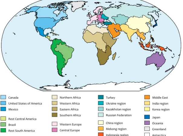
Regions in IMAGE 2.4. Source: T. Kram and E. Stehfest, 2006.

Figure 2.1 IMAGE regions

Canada

United States of America Mexico

Rest Central America Brazil

Rest South America

Northern Africa Western Africa Eastern Africa Southern Africa Western Europe Central Europe Turkey Ukraine region Kazakhstan region Russian Federation Middle East India region Korea region China region Mekong region Indonesia region Japan Oceania Greenland Antarctica Biomes in IMAGE 2.4 (MNP, 2006). Figure 2.2 IMAGE biomes, 2000 Ice Tundra Wooded tundra Boreal forest Cool coniferous forest Temperate mixed forest

Temp. deciduous forest Warm mixed forest Grassland / steppe Desert Scrubland Savanna Tropical woodland Tropical forest Mediteranean shrub

(17)

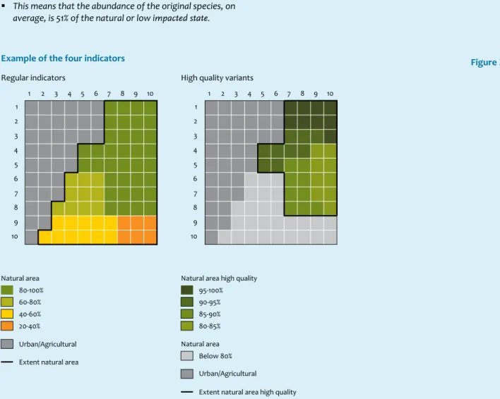
Methodology 17 The four indicators in this study are explained for a hypothetical

area of 100 cells. To keep this example simple, some classes are combined, for example, urban and agriculture areas. The first figure describes the calculation for the regular ‘natural area’ and ‘MSA’ indicators, and the second describes the ‘high quality’ (HQ) variants.

Regular indicators (left figure of Figure 2.3)

The natural area is the extent of the natural area. In this example, there are 63 ‘natural areas’ out of 100 cells; the indicator will therefore be 63%.

The MSA indicator is Quality * Area (Alkemade et al., 2009). In the example, there are 100 cells with different (average) qualities. The total MSA of the considered area is 51%, thus:

% 51 14 . 51 100 5114 100 30 * 6 50 * 11 70 * 10 90 * 36 12 * 37 * ≈ = = + + + + =

∑

A Q A

This means that the abundance of the original species, on average, is 51% of the natural or low impacted state.

High quality (HQ) variants (right figure of Figure 2.3)

The HQ indicators only consider those areas with a quality of ≥ 80%. This means that the original species have an average population (abundance) of ≥ 80% of the natural or low impacted state (‘wilderness area’).

The Natural Area HQ is the extent of the natural area with a minimum quality of 80%. In this example, 36 natural cells out of the 100 cells have a quality of ≥ 80%. Therefore, NAHQ is 36%.

The MSAHQ only considers those areas with a quality of ≥ 80%. In this example, 36 cells out of 100 cells meet this criterion, but the cells vary in quality between 80 and 100%. The MSAHQ is the high quality area (36%) times its average quality (90%), which is 32%, or more formal:

% 32 40 . 32 100 3240 100 5 . 82 * 9 5 . 87 * 9 5 . 92 * 9 5 . 97 * 9 * ≠ = = + + + =

∑

A Q AHQ HQ

Text box 1: Description of the four indicators

The applied indicators: natural area (NA) and mean species abundance (MSA).

Figure 2.3 Example of the four indicators

Regular indicators High quality variants

1 2 3 4 5 6 7 8 9 10 1 2 3 4 5 6 7 8 9 10 1 2 3 4 5 6 7 8 9 10 1 2 3 4 5 6 7 8 9 10 Urban/Agricultural Natural area

Extent natural area 80-100% 60-80% 40-60% 20-40%

Urban/Agricultural Natural area high quality

95-100% 90-95% 85-90% 80-85% Natural area Below 80%

(18)

4. “MSA high quality’ (MSAHQ) is the MSA indicator for high-quality areas (MSA > 80%). In actual practice, this means that cultivated areas are excluded and that only highly intact areas –‘wilderness’– are considered.

The high-quality (HQ) indicators prevent compensation of biodiversity loss in large, low-quality areas, such as agriculture, with damaged, incomplete ecosystems. The added value of MSA for ‘natural area’ is that it takes quality

loss into account. Please note that the Antarctic continent is excluded from all calculations.

The abovementioned indicators are ‘stock’ indicators, meaning that they describe the remaining amount of biodiversity, expressed in terms of area, and in terms of the original species and their corresponding abundances (see Figure 2.4).

The loss of biodiversity that we face today is the – generally unintentional – by-product of increasing human activity all over the world. The process of biodiversity loss, resulting from this human activity, is generally characterised by the decrease in abundance of many original species and the increase of a few other, opportunistic ones. Extinction is merely the last step in a long process of degradation. Countless local extinctions of a species (extirpations) precede a potentially final global extinc-tion. As a result, many different ecosystem types are becoming more and more alike, the so-called homogenisation process (Pauly et al., 1998; Ten Brink, 2000; Lockwood and McKinney, 2001; Scholes and Biggs, 2005; MA, 2005). Decreasing popula-tions are as much a signal of biodiversity loss as rapidly expand-ing species populations, which may sometimes even become plagues, in terms of invasions and infestations. The figure below shows this process of changing abundance (indexed) of the original species from left to right.

Until recently, it was difficult to measure the process of biodi-versity loss. ‘Species richness’ appeared to be an insufficient indicator. First, it is difficult to monitor the number of species in an area, and, more importantly, numbers may even increase as

original species are gradually replaced by new species that are favoured by humans; the so-called ‘intermediate disturbance diversity peak’. Consequently, the Convention on Biological Diversity (CBD VII/30) chose a limited set of indicators to track this degradation process, including the indicator ‘change in abundance and distribution of selected species’. This indicator has the advantage of measuring key processes, it is universally applicable, and can be measured and modelled with rela-tive ease. In the GLOBIO/MSA framework, biodiversity loss is calculated in terms of the mean species abundance of the original species (MSA) compared to the natural or low-impacted state. This baseline is used here as a means of comparing different model outputs, rather than as an absolute measure of biodi-versity. If the indicator is 100%, the biodiversity is similar to the natural or low-impacted state. If the indicator is 50%, the average abundance of the original species is 50% of the natural or low impacted state, and so on. The range of MSA values and the corresponding land use and impact levels are visualised for grassland and forest systems in Text box 3. The mean species abundance (MSA) at global and regional levels is the sum of the underlying biome values, in which each square kilometre of every biome is equally weighted (Ten Brink, 2000).

Text box 2: Process of biodiversity homogenisation expressed by the MSA indicator

Figure 2.4

abcdefgh xyz

Original species of ecosystem Natural range in intact ecosystem

Abundance of individual species, relative to natural range

Time

Process of biodiversity homogenisation expressed by the MSA indicator

MSA

0% 100%

Mean Species Abundance, relative to natural range

abcdefgh xyz

MSA

abcdefgh xyz

(19)

Methodology 19 A photographic impression of the gradual changes for two

ecosystem types (landscape level) from highly natural ecosys-tems (90 to 100% mean abundance of the original species), to

highly cultivated or deteriorated ecosystems (around 10% mean abundance of the original species).

Text box 3: A photographic impression of mean species abundance at landscape scale

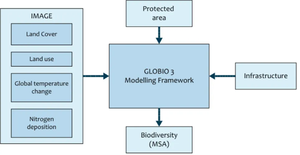
The GLOBIO model and the baseline scenario

The calculations have been made with the GLOBIO 3 framework (Alkemade et al., 2006, Alkemade et al., 2009). This modelling framework is linked with the IMAGE 2.4 model framework (MNP, 2006). GLOBIO 3 needs input data on (future) land cover, land use (i.e. pasture, crop, and forestry), protected areas, nitrogen deposition, global temperature change, and infrastructure (Figure 2.5).

We applied the Baseline scenario from the OECD Environmental Outlook to 2030 (OECD, 2008) for the years 2000 and 2050, to calculate the remaining biodiversity in 2000 and 2050 resulting from current policies and autonomous developments. The location and size of the biomes were fixed over time to make 2000 and 2050 comparable. Within the IMAGE model the biomes (slightly) shifted under the forecasted climate change.

Photographic impression of mean species abundance indicator at landscape level

Forest Mean abundance of

original species Grassland

100%

0% Pristine forest

Pristine forest Original speciesOriginal species

Selective logging Extensive use

Secondary vegetation Burning

Plantation Subsistence agriculture

(20)

Compensation scenarios

Opposite to the Baseline scenario, in the 50% compensation scenario, for 2050, we first allocated 50% of protected areas in each of the spatial units or less if this was not available (for regions, biomes, biomes per region; Figure 2.1 and Figure 2.2. Subsequently, we analysed the effect on biodiversity and whether land claims for agriculture and forestry could still be met within the remaining areas, by 2050. Two 50% compensation scenarios were constructed:

1. protected areas ‘close to nature’; 2. protected areas ‘close to agriculture’.

Nature cells were selected far from agriculture (‘close to nature’) to protect the less-disturbed nature first. In contrast, selecting nature cells close to agriculture would protect the most threatened nature first. Within these protected areas, no disrupting activities would be allowed, except for the cross-border impacts from climate change and nitrogen deposition. Current infrastructure would be continued, but agriculture and forestry were banned.

The ‘close to ..’ variants are based on maps that contain, per (half degree) raster cell, the average distance to the nearest natural or agricultural area (on a 0.0008 degree raster cell) according to the Global Land cover map for the year 2000 (GLC2000, Bartholomé and Belward, 2005). The GLC2000 natural classes ‘bare areas’ and ‘snow and ice’ are excluded from the selection procedure, based on the assumption that these areas are not directly threatened by land conversion for human use. Whether this is a valid assumption is open to discussion. Deserts, for example, have a high level of biodiversity (for example, the Namib Desert) and are

vulnerable to over-exploitation. Recently, UNEP has produced a report entirely based on global deserts (UNEP, 2006). Analyses

In the OECD Baseline scenario analysis we calculated the remaining biodiversity on four spatial units without additional

In the 50% compensation scenario analysis we projected a 50% protection option on four spatial units and calculated the effect on biodiversity and whether demands for agricultural land and forestry could still be met.

The GLOBIO 3 modelling framework (Alkemade et al. 2006).

Figure 2.5 The GLOBIO 3 modelling framework

IMAGE Land Cover Nitrogen deposition Global temperature change Land use Infrastructure GLOBIO 3 Modelling Framework Biodiversity (MSA) Protected area

(21)

Results 21

3.1 The OECD Baseline scenario

3.1.1 World (global) scale Natural area

In 2000, 68% of the global terrestrial area was natural area. In 2050, this will be 60%. Without non-productive areas1, NA

pro would shift from 62% in 2000, to 53% by 2050.

According to the Green Development Mechanism concept (GDM) there would be sufficient room for growth on the global scale. This would not be the case when only natural areas of high-quality (NAHQ) were taken into account. NAHQ will decrease from 59% to 41% by 2050. Excluding the non-productive areas, NAHQ-pro would decrease from 50% to 29% by 2050 (Table 3.1).

In 2000, humans used 40 million km2_{of the area suitable for} agricultural production (60 million km2_{) (FAO stat., 2006,} and PBL, 2008). Moreover, 10 million km2_{of land was used} as extensive grassland, unsuitable for intensive agriculture because of its low productivity. According to the Baseline scenario, the total area would grow from 50 million km2_{to 55} million km2_{by 2050; a rise of 10% with an estimated population} growth of 50% (PBL, 2008). This growth would only be feasible with an average worldwide growth in productivity of about 80%, between 2000 and 2050 (IAASTD, 2008).

MSA

In 2000, global MSA was 73%, and is expected to decline to 61%, by 2050. Without non-productive areas, MSApro1 will change from 68% in 2000 to 55% by 2050. Also in MSA terms, on a global scale, sufficient room for growth would remain, according to the GDM concept.

1 All areas excluding ice, tundra, and desert

Looking at high-quality areas, MSAHQ will decline from 55% to 37%, by 2050. Without non-productive areas, MSAHQ-pro will decline from 47% to 26% (Table 3.1).

3.1.2 Regional scale Natural area

In 2000, Central America (without Mexico), Europe (Western and Central), Turkey, Ukraine, and the India region, had less than 50% natural areas left (Table A1.1 in Appendix I). In 2050, the United States, Eastern Africa and Southern Africa are expected to join this list of ‘deficit regions’ (Table A1.1 in Appendix I). Considering only high-quality natural areas (NAHQ), 13 out of 25 regions have less than 50% remaining. In 2050, this will be 19 (Table A1.1 in Appendix I).

Excluding non-productive areas (NAHQ and NAHQ-pro), the number of ‘deficit-regions’ will be higher. Northern and Eastern Africa joined this list in 2000. In 2050, the United States, Southern Africa, Kazakhstan, and China, are also expected to join this list (Table A1.5 in Appendix I). MSA

Europe (Western and Central) and the Ukraine region had less than 50% of MSA left in 2000. In 2050, seven more regions are expected to join this list; these are the rest of Central America, Turkey, the Ukraine region, the India region, the Korea region, the Mekong region, and Japan.

Most regions with high MSA values contain large non-productive areas, such as ice, tundra, or desert. Excluding these areas, MSApro falls short for most of the areas; in 15 out of 25 regions.

Results

3

Global areas (in million km2_{) and indicator values in 2000 and for the Baseline scenario in 2050.}

World Total area<?> _NA _NA

HQ MSA MSAHQ

2000 132.84 68% 59% 73% 55%

Baseline 2050 60% 41% 61% 37%

Excluding non-productive areas

2000 99.42 62% 50% 68% 47%

Baseline 2050 53% 29% 55% 26%

(22)

For MSAHQ, 15 out of 25 regions had less than 50% of MSA, by 2000. In 2050, this is expected to be 20 regions (Table A1.1 in Appendix I). Excluding non-productive areas (MSAHQ-pro), most regions will fall short (see Table A1.8 in Appendix I).

3.1.3 Biome scale Natural area

In 2000, temperate deciduous forest, scrubland, and Mediterranean shrub, had less than 50% of natural areas remaining. These ‘deficit biomes’ were located in the wealthy, densely populated regions with much intensive agriculture. By 2050, temperate mixed forests, warm mixed forests, grassland and steppe, and savannah biomes, are expected to join the list, mostly situated in the subtropical to tropical biomes (Table A1.2 in Appendix I).

Considering the high-quality natural areas (NAHQ), the number of deficit biomes increase from 6 to 10 biomes out of 15, over the period from 2000 to 2050.

The extent of the ice biome and the tundra biomes (tundra and wooded tundra) would decline by 4% and 19%, respectively, by 20502.

MSA

Two biomes had MSA values of less than 50% in 2000. Three biomes would join the list by 2050. For MSAHQ, 7 out of 15 biomes had a value of less than 50% in 2000, and this would increase to 10 biomes, by 2050. Only ice, tundra, wooded

tundra, boreal forest and hot desert biomes, maintain values higher than 50%.

Ice is the only biome that would be relatively unaffected, by 2050 (Table A1.2 in Appendix I). The absence of agriculture and forestry keeps MSA high. Tundra biomes (tundra and wooded tundra) also would maintain high MSA values, although the area would shrink slightly, due to climate change3.

3.1.4 The scale of biome per region Natural area

In 2000, 64 out of the 190 region-biome combinations had a natural area (NA) below 50% (Table A1.3). By 2050, this number will have grown to 89 region-biome combinations. From the 126 combinations with a NA above 50% in 2000, eleven combinations had been formally protected for more than 50%. The total area of these 126 combinations was about 76 million km2_{, which is about 57% of the global area. In 2050,} this area is expected to have become 63 million km2_{(48%) and} only 101 combinations will have a NA above the 50%.

Some regions have less deficit region-biome combinations than others. Six regions were already ‘deficit regions’4 in

2000: Rest Central America, Eastern Africa, Southern Africa, Central Europe, Turkey, and the Ukraine region. In 2050

3 These area losses are not considered in the calculations. The 2000 biome location is also used in the 2050 Baseline scenario

Remaining natural areas per region. Left: all natural areas irrespective of their quality (NA). Right: hiqh-quality natural areas (NAHQ) only.

Figure 3.1

Canada United States of America Mexico Rest Central America Brazil Rest South America Northern Africa Western Africa Eastern Africa Southern Africa Western Europe Central Europe Turkey Ukraine region Kazakhstan region Russian Federation Middle East India region Korea region China region Mekong region Indonesia region Japan Oceania Greenland 0 20 40 60 80 100 Area (%) 2000 2050

All natural areas

Natural area per region

0 20 40 60 80 100

Area (%)

Natural areas with quality greater than 80% MSA

(23)

Results 23 Western Europe, the Kazakhstan region, the India region, and

the Indonesian region are expected to join this list (left figure of Figure 3.2 and Table A1.3).

For high-quality natural areas (NAHQ), 111 out of the 190 region-biome combinations had a value below 50%, in 2000. This could become 151 out of 190, by 2050 (right figure in Figure 3.2 and Table A1.3).

Excluding non-productive areas, the total number of region-biome combinations is 153. Of these, 61 had a natural area below 50% in 2000. By 2050, this could increase to 85 region-biome combinations. In area size, the abovementioned figures are 51 million km2_{and 63 million km}2_{, which is 52 and} 63%, respectively, of the ‘remaining’ global area of 99 million km2_.

MSA

In 2000 41 out of 190 region-biome combinations had a value of less than 50% MSA. This could become 99 combinations out of 190, by 2050. For high-quality areas (MSAHQ), this was 121 for the 2000 situation and could become 158 by 2050 (Table A1.3).

Excluding non-productive areas, 41 out of 153 combinations had a value of less than 50% MSA, in 2000. This could become 98 out of 153 in 2050. For high-quality areas (MSAHQ-pro), this was 116 in 2000 and 144 by 2050 (out of 153).

3.2 Two 50% compensation scenarios

As alternative scenarios, we superimposed a 50%

compensation (50% biodiversity in protected areas) on the land use map for the year 2000, disregarding land claims for other land uses. One scenario variant has a priority of protecting the most remote and highest quality natural areas, the other of protecting the most threatened areas close to current (2000) agricultural areas. Subsequently, we analysed whether sufficient agricultural land and forest would remain to cope with the food and timber demand according to the OECD Baseline scenario.

Implementing these variants per region, per biome and per biome per region, resulted in six compensation options5

(Figure 3.3). Figure 3.4 shows the differences between them. For a few regions, biomes, and especially biomes per regions, it was not possible to achieve a complete 50% protection, as this level of protection was not available in 2000. All results in the following paragraphs are for the year 2050 and are also compared with the Baseline for the year 2050.

3.2.1 Results: compensation within regions Natural area

Compared to the Baseline, for 2050, both compensation variants give better results (Table 3.2). From the nine deficit regions in the Baseline option (Table A1.1 in Appendix I), only

5 compensation on a global scale was not analysed.

Number of biomes per region with at least 50% natural areas remaining. Left: all natural areas irrespective of their quality (NA); right: high quality natural areas (NAHQ) only.

Figure 3.2

Canada United States of America Mexico Rest Central America Brazil Rest South America Northern Africa Western Africa Eastern Africa Southern Africa Western Europe Central Europe Turkey Ukraine region Kazakhstan region Russian Federation Middle East India region Korea region China region Mekong region Indonesia region Japan Oceania Greenland 0 4 8 12 16 Number of biomes Total biomes Meeting protection target

2000 2050

All natural areas

Biomes per region

0 4 8 12 16

Number of biomes

Natural areas with quality greater than 80% MSA

(24)

three regions in both compensation options (‘close to nature’ and ‘close to agriculture’) would remain ‘deficit regions’, that is, Central Europe, the Ukraine region, and the India region. Considering only high-quality natural areas (NAHQ), the number of deficit regions would be 18, this is very similar to the Baseline in which there where 19 deficit regions. But the area per region and the overall area with a high quality would be larger than in the Baseline option.

The ‘close to nature’ variant is overall the better option, although the difference with the ‘close to agriculture’ variant is small, and for a few regions the ‘close to agriculture’ variant is the better of the two.

MSA

While the Baseline option has 9 deficit regions out of 25 regions, the two compensation options have 6 (‘close to nature’ variant) or 7 (‘close to agriculture’ variant) (Table 3.2).

Six protected-area maps (‘close to nature’ and ‘close to agriculture’) per region, per biome and per biome per region combination.

Figure 3.3 Protected area options

Region close to nature Biome close to nature Region-biome combination close to nature

(25)

Results 25 region, and for the ‘close to agriculture’ variant also the Korea

region.

For MSAHQ, the deficit regions would be the same regions as the ones in the Baseline option (Table 3.2 and Table A1.1 in Appendix I). The average quality is higher.

Overall, the ‘close to nature’ variant would be the better option. Globally, MSA would be 65% for ‘close to nature’ and 64% for ‘close to agriculture’, compared to the 61% for the Baseline. The difference is larger for the MSAHQ indicator, that

is, 43% for the ‘close to nature’ variant, compared with 41% for the ‘close to agriculture’ variant.

3.2.2 Results: compensation within biomes Natural area

In both compensation variants, all biomes would have more than 50% of natural areas (NA) remaining (Table 3.3). This is significantly higher than the Baseline, by 2050, with seven ‘deficit biomes’ (Table A1.2 in Appendix I).

Six protected-area maps (‘close to nature’ and ‘close to agriculture’) per region, per biome and per biome per region combination.

Protected area options

Region close to agriculture Biome close to agriculture Region-biome combination close to agriculture Figure 3.3 continued

(26)

For high-quality natural areas (NAHQ), 10 biomes have a deficit out of 15 over the period from 2000 to 2050. This is equal to the Baseline, but the total in high quality areas would be larger in both compensation variants. The ‘close to nature’ variant has an additional seven million km2_NA

HQ, compared to the Baseline, and an additional six million km2_{for the ‘close to} agriculture’ variant.

Overall, the ‘close to nature’ variant would be the better option. Not in the number of biomes with sufficient area to

MSA

In the Baseline there are five deficit biomes, in the two compensation variants there are four: temperate mixed forest, temperate deciduous forest, warm mixed forest, and the Mediterranean shrub biome.

For MSAHQ, the deficit biomes are the same biomes as in the Baseline option (Table 3.3 and Table A1.2 in Appendix I), although their average quality is higher.

Similarities and differences between the protected area allocation approaches on three scales.

Figure 3.4 Similarities and diﬀerences between protected area allocations

Both options Close to agriculture option Close to nature option Biome differences: close to nature close to agriculture Region differences: close to nature close to agriculture Region-biome combination differences: close to nature close to agriculture

(27)

Results 27 indicator is on average higher for the ‘close to nature’ variant,

while the MSAHQ indicator is on average higher for the ‘close to agriculture’ variant.

Indicator values for compensation within regions

Region close to nature Region close to agriculture

Region Area NA NAHQ MSA MSAHQ NA NAHQ MSA MSAHQ

Canada 9.5 85 74 80 69 85 80 81 73

USA 9.3 50 32 55 28 52 28 54 24

Mexico 2.0 55 23 57 20 55 16 57 14

Rest Central America 0.7 50 41 52 35 50 32 50 27

Brazil 8.4 64 49 64 43 65 44 63 39

Rest South America 9.2 61 46 63 40 61 40 62 35

Northern Africa 5.7 87 71 81 64 87 71 81 64 Western Africa 11.3 72 55 69 49 70 51 68 46 Eastern Africa 5.8 66 42 65 37 65 38 63 33 Southern Africa 6.8 50 39 61 33 50 30 62 25 Western Europe 3.7 53 29 49 25 52 18 46 16 Central Europe 1.4 44 12 40 9 44 12 40 9 Turkey 0.8 50 1 47 1 50 1 47 1 Ukraine region 0.8 27 2 30 2 27 2 30 2 Kazakhstan region 3.9 58 29 57 24 58 29 57 24 Russian Federation 16.9 79 64 74 58 80 66 75 60 Middle East 5.1 86 61 75 55 86 61 75 55 India region 5.1 45 15 37 13 45 15 37 13 Korea region 0.2 56 46 50 38 53 36 49 30 China region 10.9 59 40 58 35 57 33 57 30 Mekong region 2.5 54 20 44 17 53 18 43 15 Indonesia region 2.3 61 48 57 42 61 44 56 38 Japan 0.4 81 18 52 15 81 13 52 10 Oceania 7.9 69 56 70 50 69 53 71 47 Greenland 2.2 100 99 97 96 100 99 97 96 World 132.8 67 48 65 43 66 46 64 41

Footnote: Indicator values (area in million km2_{, NA and MSA indicators in %) for the compensation option within regions and the}

two variants, ‘close to nature’ and ‘close to agriculture’

Table 3.2

Indicator values for compensation within biomes

Biome close to nature Biome close to agriculture

Description Area NA NAHQ MSA MSAHQ NA NAHQ MSA MSAHQ

Ice 2.3 100 100 98 97 100 100 98 97

Tundra 6.4 91 84 86 78 95 90 88 82

Wooded tundra 2.6 80 71 79 66 81 74 79 68

Boreal forest 17.6 77 68 77 63 81 75 79 68

Cool coniferous forest 3.1 66 43 57 36 74 39 60 33

Temperate mixed forest 5.9 53 31 48 26 55 26 48 21

Temperate deciduous forest 4.7 53 4 39 3 52 4 38 3

Warm mixed forest 5.8 54 21 45 18 52 17 42 14

Grassland and steppe 19.1 59 33 57 28 55 27 57 23

Hot desert 22.2 86 77 82 70 85 77 82 70 Scrubland 8.8 50 17 52 14 53 13 53 11 Savannah 15.6 55 32 56 27 54 26 55 22 Tropical woodland 7.9 59 43 58 38 58 40 57 35 Tropical forest 9.2 62 50 62 44 59 49 62 43 Mediterranean shrub 1.7 51 3 47 3 54 3 48 2 World 132.8 67 48 64 43 67 47 65 42

Footnote: Indicator values (area in million km2_{, NA and MSA indicators in %) for the compensation option within biomes and the}

two variants, ‘close to nature’ and ‘close to agriculture’

(28)

3.2.3 Results: compensation within biomes per region Natural area

In 2000, there was 68% of natural area left in the world (90.34 million km2_{). In the Baseline without extra protected} areas, this is expected to be about 60%, an extra loss of 10 million km2_{(Table 3.4). The two region-biome options would} reduce the loss with 6 million km2_{, leaving 65% natural areas} remaining (Table 3.4). Excluding the non-productive areas, the natural area would be 61% (Baseline 53%), and for the two options this would be 59%.

Only selecting high quality areas NAHQ, would result in less than 50%, and a significant part of these areas would be non-productive.

MSA

The MSA values also showed an overall decline in remaining quality (Table 3.4), from 73% MSA in the 2000 situation, to 61% in the Baseline by 2050. Implementing the region-biome options would increase the latter value to 64%. Excluding non-productive areas, the total loss in MSA with respect to the 2000 situation would vary between 13 and 10% points. The differences between the options are more pronounced when looking at the high quality MSA (MSAHQ). The loss is bigger and the ‘close to nature’ variant scores one percentage point higher.

3.2.4 Remaining claims

agriculture and forestry would increase from almost 0% to between 12 - 17% of the total land-use claim. The model run did not explore trade options between regions to cope with this, nor did it explore options of higher production efficiency. These and other interesting dynamic responses could be looked at with the IMAGE-GTAP model combination, at some time in the future. As a first check, we looked at uncultivated forest land in other regions and matched this against the not awarded wood claim. Initially, the area of non-used forest seemed to be sufficient to fulfil the remaining demand, although wood could be of a different quality and the forest productivity could be different. Russia, and, to a lesser extent, Canada, Brazil, and the rest of South America have the largest area of ‘non-used’ forest. In the Indonesia region, almost all forest areas will either be used for forestry or protected for compensation.

Global indicator values for compensation within biome per region

World total area NA NAHQ MSA MSA HQ

2000 132.8 68 59 73 55

Baseline 2050 60 41 61 37

Region-biome ‘close to nature’ 2050 65 47 64 42

Region-biome ‘close to agriculture’ 2050 65 45 64 41

Excluding non-productive areas

2000 99.4 62 50 68 47

Baseline 2050 53 29 55 26

Region-biome ‘close to nature’ 2050 59 37 58 32

Region-biome ‘close to agriculture’ 2050 59 35 58 31

Footnote: Global indicator values (area in million km2_{, NA and MSA indicators in %) resulting from compensation within biome}

per region for two variants, ‘close to nature’ and ‘close to agriculture’.

Total land claim, not awarded claims, and compensation areas (all in million km2)

Claim Not awarded claim Compensation area

Scenario 52.0

OECD Baseline 2050 0.2 19.4

Region ‘close to nature’ 8.2 62.5

Region ‘close to agriculture’ 7.7 62.5

Biome ‘close to nature’ 9.0 62.8

Biome ‘close to agriculture’ 8.8 62.8

Region-biome ‘close to nature’ 6.3 60.1

Region-biome ‘close to agriculture’ 6.1 60.2 Footnote: Total land claims for crops, pasture and wood (forest), and not awarded claim (in million km2_{) for the different 50%}

compensation scenarios.

(29)

Conclusions 29 Compensation on the global scale is possible, but has limited

effect on the average global biodiversity, in terms of mean species abundance (MSA). Though Compensation within regions or biomes will have significant effect on overall global biodiversity. Compensation on smaller scales will not improve this result, but would provide a better representativeness. Fifty percent compensation is not always feasible, given the current land use and future needs, and would result in deficits for meeting human demands by 2050 in several regions. However, these deficits could initiate increasing production efficiency, which is a primary goal of the Green Development Mechanism.

Development according to the OECD Baseline scenario Even today, it is not possible to implement a full 50% compensation regime for all regions or biomes, let alone for each biome per region. Many natural areas have already been converted in the past, leaving insufficient room for compensation. These deficits are expected to grow in the future because of socio-economic development, and when compensation is applied to smaller spatial units. If minimum quality levels (MSAHQ) are applied, or non-productive areas are excluded from compensation, the deficit will grow bigger. Development according to six compensation options According to the Baseline Scenario, the global MSA will be 61.4%, by 2050. The six 50% compensation options give a global MSA of between 64.0 and 64.8%, which is an increase of about three percentage points (Table 4.1). The amount of avoided biodiversity loss is comparable with changing an area of pristine (undisturbed) nature the size of Western Europe into a paved car park.

In the ‘biomes per region’ options, the total amount of compensated land is 60.1 million km2

. This is less than in the compensation option ‘per region’ (62.5 million km2_{) or ‘per} biome’ (62.8 million km2_{). However, the representativeness} (number of region-biome combinations above the target) of biodiversity is significantly higher (Table 4.1, right column). Figure 4.1 clearly shows the advantages of the option of ‘region per biome’ compared to the Baseline scenario. The number of ‘region-region combinations’ that achieve the 50% compensation is higher, both in terms of MSA and MSA HQ. In the compensation options, not all claims can be awarded, see Section 3.2.4. If the deficit in land for agriculture and forestry would be compensated elsewhere (in the ‘free space’) than positive effects of the compensation options would vanish on the global scale (Table 4.1, column ‘corrected MSA for remaining claim’).

Compensation does favour biodiversity, +3% compared to the Baseline scenario, in case agriculture and forestry deficits are solved by efficiency growth, instead of being compensated elsewhere. Compensation at the level of smaller spatial units does not make a difference for biodiversity on a global scale, but, looking more closely, we found that:

Conclusions

4

MSA values for 2000, Baseline 2050, and the six compensation options

Scenario MSA corrected MSA for remaining claim

# region-biome combina-tions ≥ 50% target (maximum is 190)

2000 73.0% 73.0% 126

OECD Baseline 2050 61.4% 61.3% 101

Region ‘close to nature’ 64.6% 61.2% 129

Region ‘close to agriculture’ 64.4% 61.2% 145

Biome ‘close to nature’ 64.4% 60.2% 117

Biome ‘close to agriculture’ 64.8% 61.2% 145

Region-Biome ‘close to nature’ 64.1% 61.6% 167

Region-Biome ‘close to agriculture’ 64.0% 61.6% 167 Footnote: MSA values for 2000, the Baseline by 2050, and the six compensation options (left); MSA value if not awarded claims are met elsewhere by 2050 (middle); and the number of region-biome combinations above the 50% value.

(30)

1. The high-quality area (NAHQ) will increase, while the area with a moderate quality will decrease (Figure 4.3). 2. Agriculture and forestry are more concentrated near

non-protected areas, instead of being scattered over a larger area. Given the area constrains, this might initiate intensification, which is a primary goal of the GDM concept.

3. The geographical distribution of MSA and MSAHQ changes (Figure 4.2 and Figure 13). The smaller the spatial unit

4. MSAHQ areas will contain more complete ecosystems with possibly less risk of species extinction. The improved representation would enforce this.

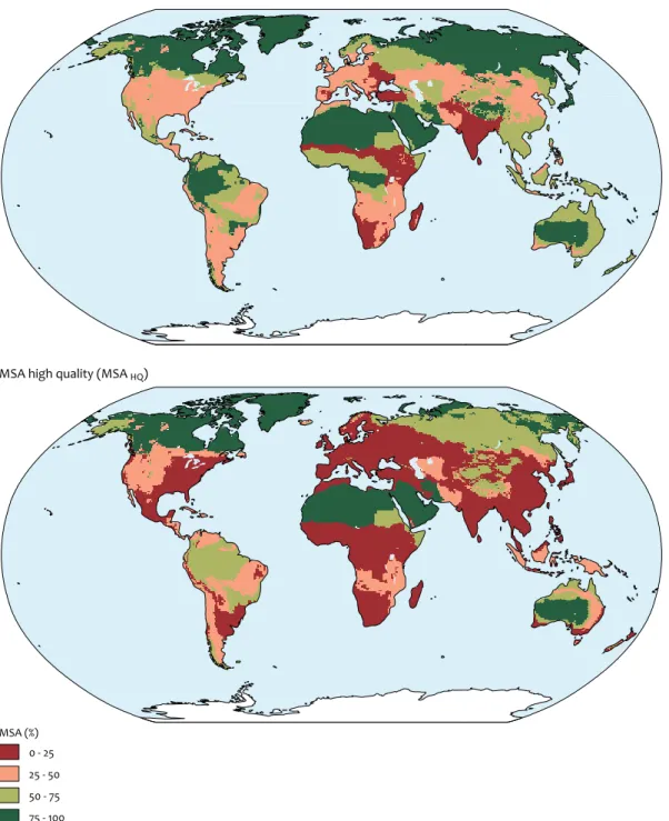
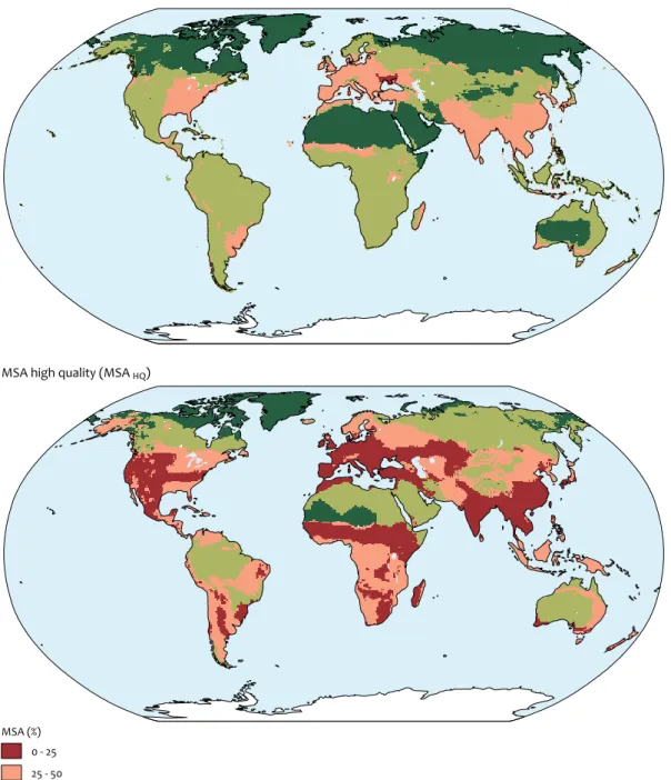
Remaining MSA in biomes per region in the Baseline scenario (left), and in the 50% compensation option ‘biome per region’ ‘close to nature’ option (right). The upper figure is in MSA; the lower figure is in MSAHQ.

Figure 4.1 Biomes per region 'at risk' in Baseline 2050

Mean species abundance (MSA)

MSA (%) 0 - 25 25 - 50 50 - 75 75 - 100

(31)

Conclusions 31 Remaining MSA in biomes per region in the Baseline scenario (left), and in the 50% compensation option ‘biome per

region’ ‘close to nature’ option (right). The upper figure is in MSA; the lower figure is in MSAHQ. Biomes per region 'at risk' in compensation option biome per region

Mean species abundance (MSA)

MSA (%) 0 - 25 25 - 50 50 - 75 75 - 100

MSA high quality (MSA HQ)

(32)

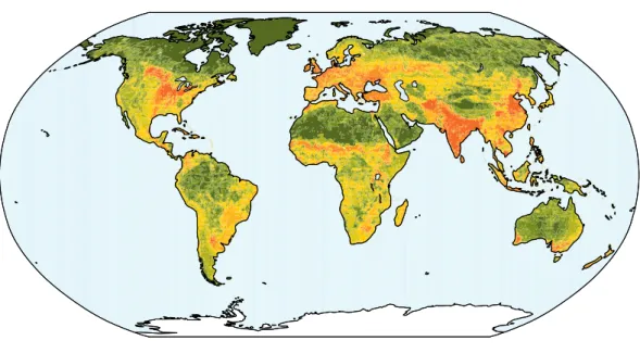
MSA maps for four different options in 2050; first map: OECD Baseline scenario (15% protected), second map: compensation per biome (‘close to nature’), third map: compensation per region (‘close to nature’), and fourth map: compensation per biome-region combination (‘close to nature’).

Figure 4.2 Mean species abundance (MSA) per option in 2050

OECD Baseline scenario

MSA

0 100

(33)

Conclusions 33 MSA maps for four different options in 2050; first map: OECD Baseline scenario (15% protected), second map:

compensation per biome (‘close to nature’), third map: compensation per region (‘close to nature’), and fourth map: compensation per biome-region combination (‘close to nature’).

Mean species abundance (MSA) per option in 2050

Compensation per region ‘close to nature’

Compensation per region-biome combination ‘close to nature’

MSA

0 100

(34)

Remaining biodiversity (MSA) in quality classes, for the OECD Baseline 2050 and the six compensation options: region ‘close to nature’, region ‘close to agriculture’; biome ‘close to nature’; biome ‘close to agriculture’, region-biome ‘close to nature’, and region-region-biome ‘close to agriculture’.

Figure 4.3 OECD Baseline 0 20 40 60 80

Mean species abundance (MSA) 0 - 20% 20 - 40% 40 - 60% 60 - 80% 80 - 100% OECD Baseline

Global distribution of biodiversity quality in 2050

Close to

nature agricultureClose to 0

20 40 60 80

Region - Biome

Close to

20 40 60 80

Biome

Close to

20 40 60 80

(35)

Discussion 35 Limitations of the study

A global MSA value can be achieved by completely different spatial configurations. On the one extreme: everywhere the same low average MSA value. On the other extreme: areas with 100% quality (hotspots) next to almost zero quality agricultural and urban areas. From a conservation perspec-tive, the second option may be more preferable as it would result in less species becoming extinct. A red list indicator of threatened and endangered species cannot yet be calculated with the GLOBIO model, but we consider MSAHQ as a prelimi-nary proxy.

From the policy-instrument perspective, the implementa-tion of this GDM concept could initiate increasing producimplementa-tion efficiency and avoiding unnecessary loss. However, within this study we could not analyse the effects of the GDM on agricultural intensification. We kept food production effi-ciency and total agricultural land claims at the same level. A new run of the IMAGE-GTAP model would be required, taking the answers to the following questions into account. Will compensation lead to intensification of agricultural practices? Will the same amount of food and wood be produced to meet the global and regional demand? In which regions will agricul-tural intensification be possible, and in which regions not? The Green Development Mechanism is likely to result in higher land prices and higher efficiency in food production.

To guarantee a global 50% protection, it would sometimes be necessary to search outside the compensation unit whenever this level of 50% is not available. This hasn’t been done in this study.

Questions

Key decisions that need to be taken are on i) the spatial units of compensation, ii) the compensation level (50%, or more, or less), iii) the indicator choice, and iv) the minimum quality level of nature acceptable for compensation (NAHQ-20%, NAHQ-50%, or NAHQ-80%). Figure 5.1 shows the effect of using natural areas with a minimum quality (NA) of 50 to 90% for compensation. Around 60% of the global area has a biodiversity quality (MSA) of between 50 and 80%. Less than 50% of the global area has a quality higher than 90%; most of these areas are non-pro-ductive areas. It is obvious that the smaller the spatial units of compensation are, the longer the ‘red list’ of ecosystems at risk will be, as shown in Figure 4.1.

In these analyses, we excluded any human use of protected areas. It is possible to include limited use of protected areas, although this would require a larger compensation area. Many questions about this type of GDM concept have not been answered, yet. This analysis is not about which biodiver-sity would be qualified to protect, or how to protect

biodi-Discussion

5

Percentage remaining natural area (NA) with a quality of ≥ 50, 60, 70, 80 or 90% in 2000 (excl. the Antarctic).

Figure 5.1 MSA greater than 50% MSA greater than 60% MSA greater than 70% MSA greater than 80% MSA greater than 90% 0 20 40 60 80

Remaining natural area with a certain minimum quality, OECD Baseline 2000

(36)

versity, nor is it about how people should be compensated and by whom, what the cost would be, or how this could be organised (see Blom et al., 2008). In this study, we have not worked out the socio-economic or cultural aspects, nor have we analysed the similarities and dissimilarities between the GDM and the Clean Development Mechanism.

The question of which biodiversity would be worth protect-ing, and which would not, has many layers and sub-questions to be answered by politicians. Contrary to CO2 compensa-tion, where every molecule of atmospheric CO2 is equal and (reduction) measures have (positive) effects everywhere, biodiversity is generally unequal, and effects are nowhere the same. This raises the question whether biodiversity (loss) somewhere can be compensated with biodiversity (gain) else-where? Moreover, would it be possible to trade in biodiversity shares (e.g., see Blom et al., 2008)?

Will implementation of a Green Development Mechanism result in a slowing down or halting of economic development in some regions, if they reach or have already exceeded the physical limitations of their ‘free’ area and compensation is beyond their reach? Or will it stimulate economic growth within particular biophysical limits by innovation and effi-ciency increase?

(37)

Tables 37

Appendix 1 Tables

The areas (in million km2_{) and indicator values (in %) per region in 2000 and the Baseline scenario 2050}

2000 2050

IMAGE region Total area Protected area NA NAHQ MSA MSAHQ NA NAHQ MSA MSAHQ

Canada 9.5 0.8 89 85 88 82 85 74 80 69

USA 9.2 2.5 56 43 63 40 49 27 52 24

Mexico 2.0 0.1 56 47 66 43 55 17 53 14

Rest Central America 0.7 0.2 44 39 59 35 45 26 46 22

Brazil 8.4 2.2 65 59 75 56 64 45 65 41

Rest South America 9.2 1.7 65 56 73 53 60 38 62 33

Northern Africa 5.7 0.4 86 83 85 78 86 76 81 70 Western Africa 11.3 1.4 71 64 78 60 61 34 63 31 Eastern Africa 5.8 0.5 57 52 73 49 33 26 55 23 Southern Africa 6.8 1.4 53 49 73 46 27 20 55 17 Western Europe 3.7 0.5 48 27 49 24 41 10 38 9 Central Europe 1.4 0.2 36 18 42 16 29 3 30 3 Turkey 0.8 0.0 38 32 51 27 2 0 25 0 Ukraine region 0.8 0.0 26 15 36 13 16 1 27 1 Kazakhstan region 3.9 0.1 66 48 67 44 56 26 53 23 Russian Federation 16.9 1.8 83 75 83 72 79 59 74 55 Middle East 5.1 0.8 83 76 81 71 86 64 75 58 India region 5.1 0.3 47 34 50 31 17 9 24 8 Korea region 0.2 0.0 74 53 62 46 53 4 38 3 China region 10.9 1.8 58 39 64 37 55 31 54 28 Mekong region 2.5 0.3 60 41 58 38 50 9 38 8 Indonesia region 2.3 0.3 68 60 71 56 60 24 52 21 Japan 0.4 0.1 71 18 53 16 82 6 44 5 Oceania 7.9 0.9 75 68 78 64 69 53 70 48 Greenland 2.2 0.9 100 99 98 97 100 99 97 96 World 132.8 19.4 68 59 73 55 60 41 61 37 World MSA 73 61 Table A1.1

(38)

Number of biomes per region with indicator values above 50% in 2000 and the Baseline scenario 2050

Number of biomes with indicator value above 50%

2000 2050

IMAGE region Total area #biomes NA NAHQ MSA MSAHQ NA NAHQ MSA MSAHQ

Canada 9.5 8 7 7 7 6 7 4 7 4

USA 9.2 15 10 6 12 5 8 4 8 4

Mexico 2.0 8 4 3 8 2 4 0 5 0

Rest Central America 0.7 5 1 0 3 0 1 0 1 0

Brazil 8.4 6 4 2 6 2 4 2 4 1

Rest South America 9.2 13 9 8 13 8 8 5 11 2

Northern Africa 5.7 3 2 1 2 1 2 1 2 1 Western Africa 11.3 7 5 5 7 4 5 1 5 1 Eastern Africa 5.8 7 2 2 6 1 1 1 2 1 Southern Africa 6.8 9 4 3 9 3 0 0 5 0 Western Europe 3.7 12 7 3 7 3 5 2 5 2 Central Europe 1.4 8 2 1 2 1 1 1 1 0 Turkey 0.8 6 0 0 2 0 0 0 0 0 Ukraine region 0.8 4 1 1 1 1 1 0 1 0 Kazakhstan region 3.9 7 5 4 5 3 3 1 4 1 Russian Federation 16.9 9 7 6 8 5 7 4 5 4 Middle East 5.1 4 4 1 4 1 4 1 2 1 India region 5.1 13 9 4 8 4 2 0 2 0 Korea region 0.2 4 4 3 3 1 3 0 0 0 China region 10.9 12 10 5 10 5 9 3 6 3 Mekong region 2.5 6 6 2 6 2 5 1 2 1 Indonesia region 2.3 3 3 1 3 1 1 0 1 0 Japan 0.4 6 6 2 3 2 6 1 2 1 Oceania 7.9 11 10 6 10 5 10 4 6 2 Greenland 2.2 4 4 3 4 3 4 3 4 3 World 132.8 190 126 79 149 69 101 39 91 32 Table A1.3 Areas (in million km2_{) and indicator values (in %) per biome in 2000 and the Baseline scenario 2050}

2000 2050

Biome Total area protected NA NAHQ MSA MSAHQ NA NAHQ MSA MSAHQ

Ice 2.3 0.9 100 100 98 98 100 100 98 98

Tundra 6.4 1.5 94 91 93 88 93 87 87 80

Wooded tundra 2.6 0.5 93 84 90 82 83 72 81 68

Boreal forest 17.6 2.3 86 81 88 79 81 69 79 64

Cool coniferous forest 3.1 0.3 73 54 68 50 66 24 55 21

Temperate mixed forest 5.9 0.7 51 30 51 27 42 10 39 9

Temperate

de-ciduous forest 4.7 0.7 45 14 42 13 39 2 31 2 Warm mixed forest 5.8 0.6 54 24 53 21 44 9 39 8

Grassland and steppe 19.1 2.1 50 38 62 35 42 21 50 19

Hot desert 22.2 2.3 83 82 87 78 76 69 79 64 Scrubland 8.8 0.9 44 39 61 36 33 13 45 11 Savanna 15.6 2.7 58 50 69 46 42 20 51 17 Tropical woodland 7.9 1.6 68 56 71 52 63 35 58 31 Tropical forest 9.1 2.0 77 70 78 66 72 42 64 38 Mediterranean shrub 1.7 0.2 39 28 49 25 35 4 37 3 World 132.8 19.4 68 59 73 55 60 41 61 37 World MSA 73 61 Table A1.2

(39)

Tables 39

Number of biomes per region with indicators ≥50% in Baseline scenario 2050 and region-biome compensation

2050 ‘close to nature’region-biome ‘close to agriculture’region-biome # meeting criteria # meeting criteria # meeting criteria

IMAGE region # biomes NA NAHQ NA NAHQ NA NAHQ

Canada 8 7 4 8 4 8 4

USA 15 8 4 15 4 15 3

Mexico 8 4 0 8 0 8 0

Rest Central America 5 1 0 4 0 4 0

Brazil 6 4 2 6 2 6 2

Rest South America 13 8 5 13 4 13 3

Northern Africa 3 2 1 3 1 3 1 Western Africa 7 5 1 6 1 6 1 Eastern Africa 7 1 1 7 1 7 1 Southern Africa 9 0 0 9 1 9 1 Western Europe 12 5 2 10 3 10 2 Central Europe 8 1 1 4 1 4 1 Turkey 6 0 0 5 0 5 0 Ukraine region 4 1 0 1 0 1 0 Kazakhstan region 7 3 1 5 1 5 1 Russian Federation 9 7 4 7 4 7 4 Middle East 4 4 1 4 1 4 1 India region 13 2 0 8 1 8 1 Korea region 4 3 0 3 2 3 1 China region 12 9 3 12 3 12 3 Mekong region 6 5 1 6 1 6 1 Indonesia region 3 1 0 3 0 3 0 Japan 6 6 1 6 1 6 1 Oceania 11 10 4 10 5 10 4 Greenland 4 4 3 4 4 4 4 World 190 101 39 167 45 167 40 Table A1.4

(40)

Indicator values per region, in 2000 and Baseline scenario 2050, excluding non-productive areas

2000 2050

IMAGE region total area NA NAHQ MSA MSAHQ NA NAHQ MSA MSAHQ

Canada 6.3 84 77 84 75 79 62 74 58

USA 8.5 53 39 60 36 46 22 50 20

Mexico 1.7 57 47 65 42 55 12 51 10

Rest Central America 0.7 44 39 59 35 45 26 46 22

Brazil 8.4 65 59 75 56 64 45 65 41

Rest South America 8.8 65 56 73 53 60 37 62 33

Northern Africa 0.7 43 29 52 26 45 10 44 9 Western Africa 7.9 64 53 72 49 55 16 53 14 Eastern Africa 4.1 47 40 67 38 23 13 46 11 Southern Africa 6.1 56 51 74 48 28 20 54 17 Western Europe 3.5 45 23 47 21 37 6 36 5 Central Europe 1.4 36 18 42 16 29 3 30 3 Turkey 0.8 38 32 51 27 2 0 25 0 Ukraine region 0.8 26 15 36 13 16 1 27 1 Kazakhstan region 2.7 60 34 60 32 49 17 48 15 Russian Federation 14.1 80 72 81 69 76 55 72 50 Middle East 1.0 64 35 57 32 66 14 48 12 India region 4.1 39 24 43 21 12 3 20 3 Korea region 0.2 74 53 62 46 53 4 38 3 China region 7.8 51 27 56 25 49 18 45 16 Mekong region 2.5 60 41 58 38 50 9 38 8 Indonesia region 2.3 68 60 71 56 60 24 52 21 Japan 0.4 71 18 53 16 82 6 44 5 Oceania 4.7 67 57 71 53 62 37 61 32 Greenland 0.0 100 0 64 0 100 6 66 5 World 99.4 62 50 68 47 53 29 55 26