Fatigue assessment of a steel truss bridge based on multi-dimensional finite element modelling

multi-dimensional finite element modelling

Academic year 2019-2020

Master of Science in Civil Engineering

Master's dissertation submitted in order to obtain the academic degree of Counsellor: Kris Hectors

Supervisors: Prof. dr. ir. Wim De Waele, Prof. dr. ir. Hans De Backer Student number: 01303682

Confidential up to and including 31/05/2030 Important

This master dissertation contains confidential information and/or confidential research results proprietary to Ghent University or third parties. It is strictly forbidden to publish,

cite or make public in any way this master’s dissertation or any part thereof without the express written permission of Ghent University. Under no circumstance may this master dissertation be communicated to or put at the disposal of third parties. Photocopying or duplicating it in any other way is strictly prohibited. Disregarding the confidential nature

of this master dissertation may cause irremediable damage to Ghent University. The stipulations mentioned above are in force until the embargo date.

multi-dimensional finite element modelling

Academic year 2019-2020

Master of Science in Civil Engineering

Master's dissertation submitted in order to obtain the academic degree of Counsellor: Kris Hectors

Supervisors: Prof. dr. ir. Wim De Waele, Prof. dr. ir. Hans De Backer Student number: 01303682

I would like to thank a number of people who were essential in the completion of this master’s dissertation.

First and foremost, I would like to express my gratitude to my supervisors prof. dr. ir. Wim De Waele and prof. dr. ir. Hans De Backer for their expert guidance throughout the year. Their support and interest in the subject steered me towards multiple interesting research angles, which aided me in delivering a scientifically relevant dissertation.

Secondly, I would like to express my sincere thanks to my counsellor, ing. Kris Hectors. Right from the start of this dissertation, he provided me with continuous feedback and support. His commitment to the project was crucial in every part of this work and was strongly appreciated.

Furthermore, I would also like to thank Didier Van de Velde and Zohra Van Damme from Infrabel. Aside from providing useful data, the site visit of the Temse bridge added an interesting practical element to this dissertation.

Lastly, I would like to thank my family and friends for their ongoing support, not only for this dissertation, but throughout the entirety of my engineering studies.

The author gives permission to make this master dissertation available for consultation and to copy parts of this master dissertation for personal use. In all cases of other use, the copyright terms have to be respected, in particular with regard to the obligation to state explicitly the source when quoting results from this master dissertation.

COVID-19 preamble

The original goal of the research in this master’s dissertation was to establish a method-ology for the fatigue assessment of railway bridges based on the case study of the Temse Bridge. This methodology consists of the development of a multi-dimensional numerical model. With the results obtained from the finite element model, a fatigue assessment can be performed. In addition to the numerical approach, a measuring campaign of the bridge was planned in March 2020. The data obtained from this measuring campaign could then be used to validate the finite element model.

Because of the COVID-19 measures which were instated on the 17th of March, the in-strumentation of the Temse bridge could no longer be done in the time frame of this dissertation. Therefore, the student was only involved in the preparation of the measure-ment campaign. As no measuremeasure-ment data was available, the numerical model could not be validated.

This preamble was written in consultation with the student and the promotors and ac-cepted by both parties.

This dissertation presents a methodology for the fatigue assessment of welded railway bridges. The methodology is developed based on a case study of the Temse bridge in Belgium, and makes use of a multi-dimensional finite element modelling approach. First, the different options concerning multi-dimensional modelling are studied, from which the submodelling approach is chosen. Next, a global model is developed, in which the fatigue loads for railway traffic from Eurocode 1 are implemented. The analysis of the global behaviour of the bridge is followed by the identification of a critical location prone to fatigue and a first fatigue assessment based on nominal stresses. Furthermore, the results from the global model are used as boundary conditions for the detailed submodel of the critical location. Including the detailed connection geometry in the submodel allows to perform a fatigue assessment based on hot spot stresses. The hot spot stresses are calculated with a numerical fatigue framework. From the fatigue assessments based on nominal and hot spot stresses, the locations most prone to fatigue in the structure can be identified. By implementing this methodology for other welded railway bridges, engineers are able to make more informed, and therefore more efficient, decisions about the maintenance of these bridges. This in turn contributes to the safe continuation of the use of ageing bridge infrastructure.

Key words: fatigue assessment, hot spot stresses, nominal stresses, steel railway bridges, multi-dimensional modelling

multi-dimensional finite element modelling

Lien Saelens

Supervisor(s): prof. dr. ir. Wim De Waele, prof. dr. ir. Hans De Backer, ing. Kris Hectors Abstract— This dissertation presents a methodology for the fatigue

as-sessment of welded railway bridges. The methodology is developed based on a case study of the Temse bridge in Belgium, and makes use of a multi-dimensional finite element modelling approach. First, the different options concerning multi-dimensional modelling are studied, from which the sub-modelling approach is chosen. Next, a global model is developed, in which the fatigue loads for railway traffic from Eurocode 1 are implemented. The analysis of the global behaviour of the bridge is followed by the identifi-cation of a critical loidentifi-cation prone to fatigue and a first fatigue assessment based on nominal stresses. Furthermore, the results from the global model are used as boundary conditions for the detailed submodel of the critical location. Including the detailed connection geometry in the submodel al-lows to perform a fatigue assessment based on hot spot stresses. The hot spot stresses are calculated with a numerical fatigue framework. From the fatigue assessments based on nominal and hot spot stresses, the locations most prone to fatigue in the structure can be identified. By implement-ing this methodology for other welded railway bridges, engineers are able to make more informed, and therefore more efficient, decisions about the maintenance of these bridges. This in turn contributes to the safe continu-ation of the use of ageing bridge infrastructure.

Keywords— fatigue assessment, hot spot stresses, nominal stresses, steel railway bridges, multi-dimensional modelling

I. INTRODUCTION

All over the world, authorities are dealing with an ageing bridge infrastructure. During the 1950’s and 1960’s, a surge took place in the construction of civil structures [1]. This results in the current situation where a large amount of the assets have reached a considerable age and some of the structures are reach-ing their design life. In 2003, the Sustainable Bridges project [2] uncovered that almost 70 % of the railway bridges in Europe ex-ceeds the age of 50 years. Furthermore, with the passing of time, traffic capacity and loads have increased [3]. Original lifetime calculations can therefore no longer be assumed as valid and need to be re-assessed. In 2013, a report by the Joint Research Centre of the European Union [4] attributed 38.3 % of all fail-ures of metallic bridges to fatigue failure. Keeping in mind the ageing infrastructure and the increased traffic loads, the impor-tance of fatigue failure of metallic bridges only increases over time.

In 2018, the SafeLife project was launched by SIM Flanders in collaboration with OCAS, Arcelor Mittal, Infrabel, C-Power, 24-Sea, Sentea, Soete Laboratory of UGent, and the Acoustics and Vibration Research Group of the VUB [5]. The SafeLife project is focused on large scale welded steel structures sub-jected to fatigue loading. Based on structural health monitoring, the lifetime prediction and management of these structures is studied. The types of structures that are included in the project are crane-way girders, jacket offshore platforms and railway

L. Saelens is a master student at the Civil Engineering Department, Ghent University (UGent), Gent, Belgium. E-mail: Lien.Saelens@UGent.be .

bridges. With the application of numerical tools, such as finite element models, and robust structural health monitoring proce-dures, the project aims to provide a more accurate remaining lifetime prediction of ageing infrastructure. This enables en-gineers to extend the remaining lifetime of the structures and make more informed maintenance decisions. In the context of the SafeLife project, a case study of the Temse bridge is dis-cussed. The objective is to develop a methodology in which an accurate fatigue assessment can be performed on steel railway bridges with welded components based on data extracted from a finite element model.

The Temse Bridge is a steel through-truss bridge that was origi-nally constructed in 1955. It has a total span of 365 m, and con-tains one movable segment to allow for larger vessels to pass. In 1961, the movable part of the bridge was expanded to a span of 54.4 m. For the construction of this new part, welded connec-tions were used instead of the riveted connecconnec-tions in the original construction. The fatigue assessment of the bridge will be fo-cussed on the movable part.

Figure 1 The Temse bridge [6]

II. MODELLING APPROACH

For a detailed fatigue assessment based on a finite element analysis of a specific location on a large scale structure, the ge-ometry of this location will have to be modelled with a sufficient degree of detail. This is preferably done with solid elements [7]. However, because of the size of most civil structures, it would be very computationally inefficient to model the entire structure with the same degree of detail. Therefore, a distinction needs to be made between the global and local part of the model. In terms of computational efficiency, the ideal case would be where the global part of the structure was modelled with beam elements and the local part of the structure with solid elements. Both parts would be present in the same model and would be able transfer information in two directions. For the realisation of this concept, a coupling method between beam and solid elements needs to be applied. The finite element software ABAQUS provides sev-eral options: the Multi-Point Constraint (MPC), the kinematic coupling method, the continuum distributing coupling method and the structural distributing coupling method. To make an

in-case study on a clamped IPE200 beam. The coupling meth-ods are discussed for the case of an axial load, a bending mo-ment and a torsional momo-ment. In figure 2, the multi-dimensional model with the axial load is shown. The results from the cou-pling methods are compared to those of a full solid model and an analytical calculation.

Figure 2 Multi-dimensional model of the IPE200 beam with an axial load

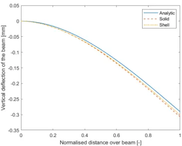
Based on the load cases of the axial load and the bending moment, viable options for the multi-dimensional coupling are the kinematic coupling (which is here equivalent to the MPC-BEAM coupling) and the continuum distributing coupling (here equivalent to the structural distributing coupling). Both coupling methods have shown results which correspond well to the refer-ence model for axial load and bending moment. However, if a torsional moment is applied in the model, both coupling meth-ods fail to capture the behaviour of the beam in a similar way as the reference model. In figure 3, the vertical deflections at the edge of the upper flange of the profile are shown.

Figure 3 Vertical deflection at upper flange of the IPE200 profile under torsion

Because of these discrepancies between the results of the cou-pling models and the reference model, it is concluded that these coupling methods cannot be applied in this context. Therefore, beam-to-solid coupling will not be used, and it is chosen to ap-ply the submodel approach in which a separate global model and submodel are developed.

III. GLOBAL MODEL

The global model is used for different purposes. First of all, the results obtained from the global model are used to iden-tify a fatigue critical location in the structure. At this location on the structure, a first fatigue assessment based on nominal stresses will be performed. Afterwards, a detailed submodel of the chosen location will be developed, for which the results of the global model will be used as boundary conditions.

is to keep the model as computationally efficient as possible. In the areas where the coupling with the submodel has to take place, shell elements are necessary. This because the submod-elling method in ABAQUS can only be applied for shell-to-solid couplings or solid-to-solid couplings. Other elements which are assumed to be less critical can be modelled with beam elements. Here, it was chosen to model the longitudinal and transverse girders as shell elements, because in practice, fatigue reinforce-ments already had to be placed in these locations. The coupling with the different parts is established by merging the parts, in which overlapping nodes of different elements are merged into one. However, for the coupling between the truss elements and transverse girders, a rigid kinematic coupling constraint is ap-plied as this better represents the connection in reality. The ex-ternal boundary conditions are modelled as hinged point con-straints in the locations on the truss elements corresponding to the real structure. The global model is meshed with quadratic beam B32 elements and quadratic shell elements with reduced integration S8R. The model is meshed with a global mesh size of 200 mm. The geometry of the global model with rendered beam sections is shown in figure 4.

Figure 4 Geometry of the global model

B. Loads

The loads implemented in the model are the fatigue loading models as described in Eurocode 1 - Part 2 [8]. For the simpli-fied fatigue approach, the LM71 load model will be used, and for a more elaborate fatigue assessment, a heavy freight traffic mix will be used. The self-weight of the structure is not included in the model, as this would only alter the mean value but not the amplitude of the stress ranges caused by the train loads. The loads are entered in the model as a sequence of static steps in which the loads are progressing over the bridge with a prede-fined step size. The load sequence is entered in the model with the user subroutine DLOAD. The distributed load is defined on a surface, namely the upper flange of the longitudinal girders. C. Identification critical detail

A number of factors are taken into account for the selection of the critical detail. These factors consist of the reporting of details prone to load-induced fatigue in literature [9], the stress results of the global model under the LM71 train load, and ob-servations made on the structure during its service life. All these factors combined lead to the decision of identifying the connec-tion between the transverse girder and longitudinal girder as the critical location. Since the highest stresses in the connection oc-cur at the mid-span of the bridge, that specific connection will

are shown in figure 5.

Figure 5 Maximal principal stresses in the global model under train load LM71

D. Fatigue assessment based on nominal stresses

Once the global model is established, stresses can be ex-tracted for the fatigue assessment based on nominal stresses. Because of the lack of a uniform stress field in the vicinity of the critical connection, several nodes are chosen from which the stresses are averaged to obtain a value which is representative for the nominal stress. Subsequently, a detail category ∆σc is

defined for the web and top flange of both the transverse and the longitudinal girder based on Eurocode 1 [8]. Because of the relative complexity of the connection, multiple detail categories are applicable, from which the most stringent ones are chosen. This results in the detail categories shown in table 1.

Table 1 Detail categories for different locations on the connection

Location Detail category ∆σc

Longitudinal girder - web 71 MPa Longitudinal girder - top flange 63 MPa Transverse girder - web 71 MPa Transverse girder - top flange 56 MPa

The fatigue assessment based on nominal stresses is per-formed with two different approaches: the stress verification ap-proach and the damage accumulation apap-proach.

1 ) Stress verification

The stress verification is performed according to the follow-ing equation:

γF f · λ · Φ · ∆σE≤

∆σc

γM f −→ ∆σE,mix/LM 71≤ ∆σR (1)

Where γF f, λ, Φ and γM f are correction factors, ∆σE is the

stress range under the fatigue loading and ∆σcis the detail

cate-gory for a specific location. A rainflow analysis is performed on the stress histories obtained from the averaged nodal stresses. This to identify the maximal stress range occurring under the different load models. A maximal stress range is defined for the traffic mix loading model and for the LM71 loading model. The stress ranges are then multiplied with the appropriate correction factors to obtain the respective ∆σE,mix and ∆σE,LM 71

val-ues. The detail classes ∆σcare divided by a γM f factor of 1.25

to obtain the ∆σRvalues. The results of these calculations are

shown in table 2.

LG - web 57.39 MPa 72.39 MPa 56.8 MPa LG - top flange 60.14 MPa 75.30 MPa 50.40 MPa TG - web 43.23 MPa 43.07 MPa 56.8 MPa TG - top flange 80.06 MPa 80.41 MPa 44.80 MPa From the results, it can be concluded that for most locations there is little to no load reserve. This could be contributed to the fact that conservative design choices may have been made, such as the value of 1.25 for γM f which implicates that failure

of the longitudinal or transverse girder would lead to rapid fail-ure of the entire bridge. One could argue that the structfail-ure with the continuous longitudinal girders is a highly statically inde-terminate structure, allowing for a lower γM f of 1.1, thereby

in-creasing the resistance values ∆σR. However, the load values of

the flange of the transverse girder would still largely exceed its resistance value. Because no specific guideline concerning the extraction of the nominal stress from a finite element model is included in the Eurocode, an additional way to obtain the nom-inal stresses from the model is used. It consists of converting the resultant forces from free body cuts to stress values. The free body cuts are each taken at a distance of 200 mm from each other. The results are shown in the graph on figure 6.

Figure 6 Stress histories for different locations of nominal stress extraction for the transverse girder

The averaged stress is taken at 200 mm from the connec-tion, position 2 is located an additional 200 mm away from the connection, and position 1 is located another 200 mm further away. The averaged stresses and the stresses at position 2 show quite a similar behaviour and magnitude. However, only 200 mm further, the maximal stress ranges are reduced to one third of the stresses closer to the connection. This would of course make a large difference in the fatigue assessment, but as no spe-cific guidelines concerning the extraction location of the nomi-nal stress are present in the Eurocodes, it is difficult to conclude which stress is more representative.

For the longitudinal girder, a similar comparison of stresses was performed, but the differences between the stresses were not as significant as for the transverse girder. The nominal stresses ex-tracted for the longitudinal girder can be assumed as representa-tive.

ing algorithm is applied to the stress histories of the nominal stresses. This results in a number of stress ranges ∆σ with a corresponding number of cycles n for each passage over the bridge of a particular train type. Only the traffic mix loading model is discussed in the context of damage accumulation, as the LM71 loading model is not correlated to a discrete number of train passages. From the recommendations in Eurocode 1 [8] concerning the number of train passages per day, and a design lifetime of 100 years, a total number of cycles can be appointed to each stress range of the train types. For each stress range, the endurance N is calculated with the S-N curves provided in Eurocode 3 [10]. With the application of the linear damage ac-cumulation rule of Palmgren-Miner, a damage value Ddcan be

calculated: Dd= n X i nEi NRi (2)

After the application of the rainflow algorithm on the stress his-tory in the web of the longitudinal girder, the histogram in figure 7 is found. From the histogram, it is clear that only one cycle exceeds the range of 0 MPa to 10 MPa. This single large cycle is attributed to the train entering and leaving the bridge. Because the cut-off limit of the web of the longitudinal girder is equal to 28.73 MPa, the stresses with a range from 0 MPa to 10 MPa will not have an influence on the damage value Dd. For the other

train types, the most relevant stress cycle also occurs during the train entering and leaving the bridge.

Figure 7 Histogram for stress cycles for train type 5 at the web of the longitudinal girder

The cycle counting algorithm and damage accumulation rule are applied for every location at the connection and for every train type. The stress histories used here are those with the av-eraged stresses mentioned in the previous section. In the calcu-lation of the damage accumucalcu-lation, the same correction factors are applied as for the stress verification. The results for the total damage value for a 100 year design life are listed in table 3.

LG - web 0.1193 LG - top flange 0.3155 TG - web 0.0576 TG - top flange 0.8906

Aside from the similarities in relative importance between the different locations, the damage accumulation approach shows a much more nuanced image of the fatigue in the critical detail. Where in the stress verification approach almost every resistance value was exceeded, none of the Dd values exceed the critical

value of unity. The flange of the transverse girder can still be identified as the relatively most critical detail.

3 ) Conclusion

With the fatigue assessment based on nominal stresses, the flange of the transverse girder was identified as the critical lo-cation. The stress verification approach showed to be much more conservative than the damage accumulation approach, as almost all resistance values were exceeded for the former, and none of the detail locations were really critical in the latter. Spe-cial points of attention are the flexibility in the hands of the de-signer in the selecting of certain correction factors, but, more importantly, the location from which the nominal stresses are extracted. Due to a lack of specific guidelines in the Eurocodes, this location is open for interpretation and can lead to very dif-ferent results.

IV. SUBMODEL

A. Geometry, boundary conditions and mesh

The geometry of the submodel consists of solid elements. The connection geometry is modelled as detailed as possible, includ-ing the weld geometries. The welds are modelled usinclud-ing triangu-lar elements. The ’seam’ tool in ABAQUS is used to ensure the separate plates are only connected by the welds and not by other possible overlapping nodes at common surfaces. The extent of the submodel is determined based on different factors. First, a thumb rule presented by Yan, Lin and Huang [11] is applied in which the submodel has to have a minimal size of four times the governing dimension of the smallest member. In this case, this dimension is equal to 220 mm, leading to a minimal size of the model of 880 mm. However, geometric issues also need to be taken into account, for example the inclusion of the cope holes and cover plates on the longitudinal girder. The final dimensions of the submodel are 975 mm by 1520 mm. No additional loads are added in the submodel, as all stresses in the connection will be obtained by the coupling with the global model. This cou-pling is established by applying the submodel boundary condi-tion to the centrelines of the longitudinal and transverse girder at the edges of the submodel. The submodel is placed in such a way that its location corresponds to its exact location in the global model. It should be noted that, since this is a repetitive detail over the length of the bridge, the submodel can be placed at other locations in the global model if necessary. The sub-model is meshed with a global mesh size of 20 mm, with local

model is shown in figure 8.

Figure 8 Meshed submodel

B. Fatigue assessment based on hot spot stresses

The detailed modelling of the connection geometry in the sub-model allows for a fatigue assessment based on hot spot stresses. Issues with the nominal stresses, such as classification of the de-tail category and location of the stress extraction, are no longer present. The fatigue (FAT) classes are described for each weld type separately, leaving almost no room for interpretation. Also, extrapolation procedures for the hot spot stresses are elaborated in the guidelines of the IIW [12], clearly indicating the extrac-tion locaextrac-tion of the stresses. For the calculaextrac-tion of the hot spot stresses, a numerical fatigue framework described in the article ”Numerical framework for fatigue lifetime prediction of com-plex welded structures” [13] is used. In the framework, a single time step can be entered in which the stresses represent a stress cycle. The fatigue spectrum is then manually composed with the possibility to scale the stress ranges and to assign a number of cycles to each stress range. In the selected critical detail, seven types of fillet welds are present which could be investigated. However, because of the ’moving’ train load and the various locations of the welds on the critical connection, the represen-tative stress cycles do not occur simultaneously for each weld. Furthermore, if the weld is oriented along the longitudinal direc-tion of the bridge, it is not possible to describe its load history with one single step as maximal stress values will occur at dif-ferent locations at difdif-ferent time steps along the weld. Because of these limitations, two welds are selected which are oriented perpendicular to the longitudinal direction of the bridge. The stress history along these welds can then be sufficiently accu-rately described by a limited number of time steps. The welds which are selected are shown on figure 9.

Figure 9 Selected welds for the fatigue assessment based on hot spot stresses

For each of the welds, a rainflow analysis is performed so that representative time steps can be selected to portray the relevant

ber of cycles, and a scale factor for the stress range. The scale factor is used to apply the correction factors as for the nomi-nal fatigue assessment, and to convert absolute stress values to the amplitude of the stress range if necessary. An extrapolation method is also chosen according to the guidelines in the IIW [12], where the extrapolation points are located at 0.5t and t for a relatively coarse mesh. With these input data, the framework is able to calculate the hot spot stresses along the length of the selected welds.

1 ) Stress verification

For the stress verification, equation 1 is again used. The dif-ference here is the use of fatigue classes instead of detail cate-gories, and that the maximal stress range is determined based on hot spot stresses instead of nominal stresses. The stress verifica-tion is performed for the traffic mix load model and the LM71 load model. The results of the stress verification are shown in table 4.

Table 4 Stress verification results based on hot spot stresses

FAT class ∆σE,LM 71 ∆σE,mix ∆σR

Weld A 90 MPa 94.45 MPa 59.91 MPa 72 MPa Weld D 100 MPa 146.66 MPa 162.32 MPa 80 MPa For weld A, an acceptable result is obtained for the loads of the traffic mix. However, for the LM71 load, the resistance is largely exceeded. The situation is more severe for weld D. To exclude the fact that the large value for weld D is caused by local peaks, the hot spot stresses are plotted along the weld in figure 10. In the contour plot of the hot spot stresses, values of 100 MPa can be observed all along the length of the weld. These values still need to be corrected with a Φ3value and a λ value,

which will lead to even larger values. Either way, weld D should be classified as a critical detail.

Figure 10 Distribution of hot spot stresses around weld D

The same considerations can be made here as for the nomi-nal stress approach. As the same correction factors have been used, there is still a possibility that overly conservative design choices have been made. The ambiguity concerning the loca-tion choice of the stress extracloca-tion is however strongly reduced, as guidelines were available at this time.

2 ) Damage accumulation

A similar damage accumulation approach is performed as for the nominal stresses, this time integrated into the framework.

a more elaborate explanation is given in those documents com-pared to the Eurocode concerning hot spot stresses. The linear damage accumulation rule of Palmgren-Miner is used to obtain Dd. The results from the damage accumulation approach are

shown in table 5.

Table 5 Accumulated damage values Ddbased on hot spot stresses

Damage Dd

Weld A 0.061 Weld D 1.495

The same trend can be observed for the results of the dam-age accumulation method compared to the stress verification method. Weld D clearly stands out as a critical detail. Weld A however, shows to be much less critical compared to the results obtained by the stress verification.

3 ) Conclusion

Compared to the fatigue assessment based on nominal stresses, much less freedom of interpretation is left in the hands of the designer. This mainly concerns the choice of FAT classes and the location of stress extraction from the model. Some con-servativeness is still allowed in the calculations, as the same cor-rection factors were used as for the submodel. Because of the clearer guidelines, more credibility can be attributed to the hot spot stress approach. The damage accumulation approach again shows to be less conservative compared to the stress verification approach, but weld D is proven to be critical in both approaches. Due to a lack of compatibility between the finite element outputs and the framework for the calculation of hot spot stresses, only a limited amount of welds could be discussed. In the future, this could be resolved by developing a matrix with scale factors for all locations of the submodel. This way, critical states for every weld could be combined into one time step.

V. CONCLUSION

In this dissertation, a methodology was developed for the fa-tigue assessment of welded railway bridges. This was done based on a multi-dimensional approach, namely by implement-ing a combination of a global model for the overall behaviour of the bridge with a submodel containing very detailed information about a critical connection. With the prescribed train loads from the Eurocode 1 [8], stress histories could be extracted from the global model, which could then be used to perform a first fa-tigue assessment based on nominal stresses. This was done with both a stress verification and damage accumulation approach, in which the damage accumulation approach showed to be less conservative. A critical detail was identified, however, ambigu-ity in the results was shown based on the location of the nominal stress extraction.

After a detailed submodel was developed, the fatigue assessment could also be performed based on hot spot stresses. A numer-ical fatigue framework [13] was used for the calculation of the hot spot stresses. Due to a different approach concerning stress histories in the finite element model and the fatigue assessment framework, only a limited number of the welds on the critical

able to use it as input for the framework as one single step. How-ever, the limited analysis still showed the possibility to appoint a critical detail concerning fatigue failure. This information al-lows engineers to implement a more optimised maintenance ap-proach.

REFERENCES

[1] Pantura, Needs for maintenance and refurbishments of bridges in urban environments p.148, 2013

[2] B. Brian, WP1, and N. Rail, Sustainable Bridges: Assessment for Future Traffic Demands and Longer Lives, WP1-02-T-040601-F Deliverable D 1.2 report on the age profile and condition of existing European railway bridges pp. 1-15, 2004.

[3] BRIME, Brime Deliverable D14, no. January 1998, p. 227, 2001. [4] B. K¨uhn, L. M., A. Nussbaumer, H. G¨unther, H. R., H. S., M. Kolstein, S.

Walbridge, B. Androic, O. Dijkstra, and O. Bucak, Assessment of existing steel structures - Recommendations for estimation of the remaining fatigue life, Procedia Engineering, vol. 66, no. February, pp. 3-11, 2013. [5] SIM-Flanders, https://www.sim-flanders.be/ Accessed on 2020-04-21 [6] C. Peelaerts, https://twitter.com/CPeelaerts/status/1114117490378977286

Accessed on 2020-04-21

[7] F. Zamiri Akhlaghi, Fatigue life assessment of welded bridge details using structural hot spot stress method - A numerical and experimental case study, tech. rep., 2009.

[8] European Committee for Standardization, Eurocode 1: Actions on struc-tures - Part 2: Traffic loads on bridges techn. rep., 2003.

[9] G. Alencar, A. de Jesus, J. G. S. da Silva, and R. Calc¸ada, Fatigue cracking of welded railway bridges: A review, Engineering Failure Analysis, vol. 104, no. May, pp. 154-176, 2019.

[10] European Committee for Standardization, Eurocode 3: Design of steel structures - Part 1-9: Fatigue, techn. rep., 2006.

[11] F. Yan, Z. Lin, and Y. Huang, Numerical Simulation of Fatigue Behavior for Cablestayed Orthotropic Steel Deck Bridges using Mixed-dimensional Coupling Method, KSCE Journal of Civil Engineering, vol. 21, no. 6, pp. 2338-2350, 2017.

[12] A. Hobbacher, IIW document IIW-1823-07: Recommendations for fatigue design of welded joints and components, techn.rep., 2008.

[13] K. Hectors, H. De Backer, M. Loccufier, and W. De Waele, Numeri-cal framework for fatigue lifetime prediction of complex welded structures, Frattura ed Integrita Strutturale, vol. 14, no. 51, pp. 552-566, 2020.

List of Figures 15

List of Tables 19

List of Abbreviations 20

List of Symbols 21

1 Introduction 22

1.1 The Temse Bridge . . . 22

2 Literature review 25 2.1 Ageing bridge infrastructure . . . 25

2.2 Bridge monitoring . . . 28

2.2.1 Historic approach . . . 28

2.2.2 Structural Health Monitoring . . . 30

2.3 Fatigue . . . 32

2.3.1 Fatigue in metallic bridges . . . 32

2.3.2 Fatigue process . . . 35

2.3.3 Fatigue assessment methods . . . 35

2.4 Finite element modelling for fatigue assessment of ageing structures . . . . 40

2.4.1 Finite element method . . . 40

2.4.2 Multi-dimensional problem . . . 41

2.4.3 Modelling welded connections . . . 47

3 Modelling approach 51 3.1 Mixed-dimensional modelling . . . 51 3.1.1 Coupling methods . . . 52 3.1.2 Axial load . . . 53 3.1.3 Bending moment . . . 57 3.1.4 Torsional moment . . . 60

3.1.5 Comparison with literature . . . 63

3.2 Choice of modelling approach . . . 63

4 Global model 64

4.1 Goals . . . 64

4.2 Geometry . . . 64

4.3 Materials . . . 69

4.4 Constraints . . . 69

4.4.1 Connections within the structure . . . 69

4.4.2 External boundary conditions . . . 71

4.5 Loads . . . 73

4.5.1 Fatigue load models in Eurocode 1 . . . 73

4.5.2 Implementing the fatigue loads in the model . . . 77

4.6 Mesh . . . 78

4.7 Dynamic analysis . . . 80

4.8 Identification of critical location . . . 82

4.9 Fatigue assessment based on nominal stresses . . . 83

4.9.1 Fatigue strength . . . 84

4.9.2 Fatigue assessment based on stress verification . . . 88

4.9.3 Fatigue assessment based on damage accumulation . . . 97

4.9.4 Conclusion . . . 102

5 Submodel 103 5.1 Geometry and constraints . . . 103

5.1.1 Modelling of the welds . . . 104

5.1.2 Submodel coupling . . . 105

5.1.3 Extent of the submodel . . . 106

5.2 Mesh . . . 107

5.3 Fatigue assessment based on hot spot stresses . . . 109

5.3.1 Fatigue strength . . . 111

5.3.2 Selection of stress ranges . . . 112

5.3.3 Fatigue assessment based on stress verification . . . 117

5.3.4 Fatigue assessment based on damage accumulation . . . 119

5.3.5 Conclusion . . . 121

6 Summary and reflection on the methodology 122

Bibliography 124

1.1 The Temse Bridge [3] . . . 23

1.2 Aerial view of the original and new Temse Bridge [4] . . . 23

2.1 Age distribution of railway bridges in Europe [11] . . . 26

2.2 Age distribution of road bridges in Europe [8] . . . 26

2.3 Age distribution of road bridges in the USA [12] . . . 27

2.4 Distribution of failure causes of collapsed metallic bridges [33] . . . 33

2.5 Distribution of failure causes of non-collapsed metallic bridges [33] . . . 34

2.6 Fatigue crack occurring at a cut-out [36] . . . 35

2.7 Fatigue crack occurring at a welded connection [37] . . . 35

2.8 Through thickness at weld method (a and b) and surface extrapolation method (c) [39] . . . 36

2.9 S-N curves provided in the Eurocode [38] . . . 37

2.10 S-N curves provided in IIW recommendations [40] . . . 37

2.11 Distribution of forces in underlying elements according to Eurocode 1 [46] . 39 2.12 Probability density function for the fatigue life of various detail classifica-tions [45] . . . 39

2.13 Element types used in Finite Element software packages [48] . . . 40

2.14 Beam model of the Tr´ezoi railway bridge [51] . . . 41

2.15 Solid model of critical location on the bridge [37] . . . 41

2.16 Nominal stresses in a beam element subjected to bending and axial force [40] 42 2.17 Mixed-dimensional modelling of the Xiangshangang bridge by using kine-matic coupling [56] . . . 44

2.18 Partial views of the global model developed by Albuquerque et al. [63] . . 46

2.19 Submodel of the railway bridge improved by Horas et al. [64] . . . 47

2.20 Weld modelling options for models consisting of shell elements. a) inclined shell elements. b) rigid links [39] . . . 48

2.21 Modelling of welded connections recommended by the IIW [40] . . . 48

2.22 Shell model with inclined shell elements [66] . . . 49

2.23 Shell model with increased shell thickness [66] . . . 49

2.24 Solid model with coarse mesh [66] . . . 50

2.25 Solid model with fine mesh [66] . . . 50

3.1 Model setup for validation of multi-dimensional coupling methods . . . 52

3.2 Application of load and boundary conditions on solid model . . . 53

3.3 Application of load and boundary conditions on mixed-dimensional model . 53 3.4 Front and side view of solid element mesh . . . 54

3.5 Comparison of reference data for axial deformation along centerline . . . . 54

3.6 Axial deformation along centerline for different coupling methods . . . 55

3.7 Axial deformation along centerline for different distributing coupling meth-ods. CD: continuum distributing coupling method, SD: structural distribut-ing coupldistribut-ing method . . . 56

3.8 Axial deformations with structural distributing coupling with cubic weight-ing function . . . 56

3.9 Comparison of reference data for vertical deflection along centerline . . . . 58

3.10 Vertical deformation along centerline of beam in bending for different cou-pling methods . . . 59

3.11 Vertical deformation along outer end of upper flange of beam in bending . 60 3.12 Comparison of reference data for rotation in longitudinal direction along centerline . . . 61

3.13 Vertical deformation of the centerline of the beam under torsion . . . 62

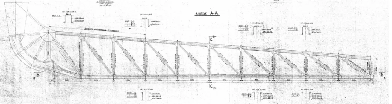
3.14 Vertical deformation along outer end of upper flange of beam under torsion 62 4.1 Side view of the main trusses of the structure . . . 65

4.2 Top view of longitudinal and transverse girders. Centrelines of the lower wind braces are drawn as well . . . 65

4.3 Top view of the upper wind braces . . . 65

4.4 Schematic representation of the different cross-sections in the main trusses 66 4.5 Different cross-sections of the main trusses . . . 67

4.6 Skin sections on the flanges of the longitudinal and transverse girder . . . . 68

4.7 Geometry of the global model . . . 68

4.8 Geometry of the global model with rendered beam profiles and shell thicknesses 69 4.9 Enlarged cross-section of the transverse girder at the connection with the truss . . . 70

4.10 Simple beam model in Scia with hinged transverse girders . . . 70

4.11 Comparison between different connections in ABAQUS based on Scia results 71 4.12 Schematic representation of external boundary conditions applied in the global model . . . 72

4.13 Connection between truss and transverse girder at pivot end . . . 72

4.14 Application of the boundary condition at the pivot support . . . 73

4.15 Traffic load model LM71 [46] . . . 74

4.16 Type 5 train load - Locomotive-hauled freight train, 225 kN axles . . . 75

4.17 Type 6 train load - Locomotive-hauled freight train, 225 kN axles . . . 75

4.18 Type 11 train load - Locomotive-hauled freight train, 250 kN axles . . . 76

4.19 Type 12 train load - Locomotive-hauled freight train, 250 kN axles . . . 76

4.21 Mesh convergence study . . . 79

4.22 Global model with a mesh size of 200 mm . . . 80

4.23 First eigenmode of the Temse bridge . . . 81

4.24 Second eigenmode of the Temse bridge . . . 81

4.25 Third eigenmode of the Temse bridge . . . 81

4.26 Maximal principal stresses [MPa] in the global model under the LM71 load 82 4.27 Location of the critical detail . . . 83

4.28 Contourplot of S11 stresses with indication of nodes used for nominal stresses 84 4.29 Side view of the detail of the connection between the longitudinal and trans-verse girder . . . 85

4.30 Detail category for welded built-up sections with start and stop positions [38] 85 4.31 Detail category for welded built-up sections with cope-holes [38] . . . 86

4.32 cross-section of the longitudinal girder in a) the support zone and b) the span zone . . . 86

4.33 Detail category for transverse butt welds with cope holes [38] . . . 87

4.34 Detail category for orthotropic bridge decks with open stringers [38] . . . . 87

4.35 Detail category for end of cover plates [38] . . . 88

4.36 Shift of the S-N curve for detail categories indicated with an asterisk [38] . 88 4.37 Flowchart concerning the necessity of a dynamic analysis [46] . . . 90

4.38 Locations for which the fatigue assessment is performed. 1: web of the longitudinal girder. 2: top flange of the longitudinal girder. 3: web of the transverse girder. 4: top flange of the transverse girder . . . 92

4.39 Stresses in the web of the longitudinal girder in the longitudinal direction for the heavy freight traffic mix . . . 93

4.40 Stresses in the web of the longitudinal girder in the longitudinal direction for the LM71 load . . . 93

4.41 Locations of free body cuts on the longitudinal girder . . . 95

4.42 Locations of free body cuts on the transverse girder . . . 95

4.43 Stress histories for different locations of nominal stress extraction for the longitudinal girder . . . 96

4.44 Stress histories for different locations of nominal stress extraction for the transverse girder . . . 97

4.45 Rainflow cycle count for train type 5 at the web of the longitudinal girder . 99 4.46 Histogram for stress cycles for train type 5 at the web of the longitudinal girder . . . 99

4.47 S-N curve for detail category 71 with indication of relevant stress range caused by train type 5 on the web of the longitudinal girder . . . 100

4.48 Adapted S-N curve for detail category 63 . . . 101

5.1 Connection detail. Left: view along the transverse girder. Right: view along the longitudinal girder . . . 103

5.2 Top view of the additional cover plates . . . 104

5.4 Example of the use of seams in the submodel . . . 105

5.5 Application of the submodel boundary condition . . . 105

5.6 Overlay plot of the submodel and the global model . . . 106

5.7 Geometry of the submodel . . . 107

5.8 Elements with bad geometry resulting from a mesh size of 10 mm by 10 mm 108 5.9 Mesh of the submodel with a global size of 20 mm . . . 109

5.10 Location of weld A . . . 109 5.11 Location of weld B . . . 109 5.12 Location of weld C . . . 110 5.13 Location of weld D . . . 110 5.14 Location of weld E . . . 110 5.15 Location of weld F . . . 110

5.16 Stress histories for the different welds under the type 5 train load . . . 111

5.17 FAT class 90 for cruciform joints with load carrying fillet welds [38] . . . . 112

5.18 FAT class 100 for cover plate ends [38] . . . 112

5.19 Histogram of stress cycles in weld A under the type 5 train load . . . 113

5.20 Stress history in weld A under the type 5 train load . . . 114

5.21 Histogram of stress cycles in weld D under the type 5 train load . . . 115

5.22 Stress history in weld D under the type 5 train load . . . 116

5.23 Distinction between ’type a’ and ’type b’ welds [40] . . . 117

5.24 Hot spot stresses at weld A under LM71 load . . . 118

5.25 Distribution of hot spot stresses around weld D . . . 119

5.26 Contourplot of maximal principal stresses around weld D under type 5 train load . . . 119

2.1 Assessment factors for LCA analysis according to Dinas, Nikolaidis and

Baniotopoulos [14] . . . 27

2.2 Condition ratings 5 to 7 provided by the Federal Highway Administration [19] 29 3.1 Total CPU times for different coupling methods . . . 57

4.1 Heavy traffic mix with 250 kN axles [46] . . . 77

4.2 Values for γM f as proposed in the Belgian National Annex [38] . . . 92

4.3 Stress verification results based on nominal stresses . . . 94

4.4 Dd values for each location at the critical connection . . . 101

5.1 Correction factors used in the stress verification based on the hot spot stresses117 5.2 Stress verification results based on hot spot stresses . . . 118

5.3 Accumulated damage values Dd based on hot spot stresses . . . 120

AASHT O American Association of State Highway and Transportation Officials BRIM E Bridge Management in Europe

CD Continuum Distributing coupling method CP U Central Processing Unit

F AT Fatigue class F E Finite Element F OS Fibre Optic Sensors LG longitudinal girder

LM 71 Load Model 71. Standard train load from EC1-2 M P C Multi-Point Constraint

N DT Non-Destructive Testing

SD Structural Distributing coupling method SHM Structural Health Monitoring

T G transverse girder W IM Weigh In Motion

A area of a cross-section E modulus of elasticity G shear modulus

I bending moment of inertia It torsion constant

Iw warping constant

LΦ determinant length of a structural member for the calculation of the dynamic factor Φ

nE number of cycles correlated to a certain stress range ∆σE N_R endurance of a structural detail for a certain stress range ∆σ_E R stress ratio for a certain stress cycle ∆σmin

∆σmax

ws wheel speed parameter, used in the DLOAD subroutine γF f partial safety factor for fatigue loading

γM f partial safety factor for fatigue strength ∆σc detail category for nominal stresses ∆σD constant amplitude fatigue limit ∆σE stress range caused by fatigue loading ∆σL cut-off limit

∆σR fatigue resistance

λ damage equivalence factor for fatigue Φ dynamic factor for traffic loads

Introduction

Ageing infrastructure is a growing problem for authorities all over the world. To ensure the safety of these assets up to their intended design lives, a proper damage assessment is needed. In 2018, SIM-Flanders initiated the SafeLife project in collaboration with OCAS, Arcelor Mittal, Infrabel, C-Power, 24-Sea, Sentea, Soete Laboratory of UGent, and the Acoustics and Vibration Research Group of the VUB. SIM-Flanders, which stands for Strategic Initiative Materials, is a virtual research group which aims to improve the sci-entific materials base and to build technology platforms in relevant areas with sufficient critical mass [1]. The SafeLife project in particular is focused on large scale welded steel structures subjected to fatigue loading. Based on structural health monitoring, the lifetime prediction and management of these structures is studied. Types of steel structures that are studied include railway bridges, crane-way girders and jacket offshore platforms. By ap-plying robust structural health monitoring procedures and using numerical tools, the goal is to obtain a more accurate remaining lifetime assessment of ageing infrastructure. The increased accuracy of the predictions enables engineers to quantify the lifetime extension of these structures and optimise predictive maintenance. The optimised approach would lead to a substantial reduction of operation and maintenance costs while maintaining the structural integrity of the ageing structures for a longer period of time.

In the context of the SafeLife project, the scope of this master’s dissertation is to develop a methodology for an accurate fatigue assessment of steel bridge structures based on a finite element model. The methodology is developed based on a case study of a steel truss bridge that is managed by Infrabel and results in a fatigue assessment in critical details based on both nominal stresses and hot spot stresses.

1.1

The Temse Bridge

The Temse bridge is a steel through-truss bridge that was built in 1955. It has a total span of 365 metres, subdivided in intermediate spans ranging from 36.85 metres to 81.7 metres. The bridge is divided into a part for railway traffic and a part for road traffic. Up to 2008, the bridge had the largest total span of all bridges in Belgium [2].

Figure 1.1: The Temse Bridge [3]

Since the bridge crosses the river Scheldt, a part of the bridge can be opened to let larger vessels pass through. The movable part of the structure is a bascule bridge and ini-tially had a span of 33.2 metres. In 1961, the movable part of the bridge was extended to facilitate the waterway traffic. The movable span was increased to 54.4 metres. While the original structure was assembled with riveted connections, welded connections were used for the construction of the new movable part. In 1997, additional plates were welded on the top flange of the longitudinal girders for reinforcement as fatigue problems had started to arise. In 2005, the Flemish government decided to build a new bridge next to the existing bridge, as the old Temse Bridge was no longer able to fulfil functional demands. Four car lanes, two in each directions, had to merge into two on the bridge, leading to daily traffic jams. The new bridge was 9 metres longer than the original bridge, thereby taking the title of longest span bridge in Belgium.

Figure 1.2: Aerial view of the original and new Temse Bridge [4]

of the project is to develop numerical and experimental methodologies to improve the understanding of the global structural behaviour and to assess the remaining fatigue life of the structure. Furthermore, the techniques and models developed in this work will also be applicable to similar civil engineering structures, thereby improving the state-of-the-art with respect to fatigue assessment of such structures. The focus of the fatigue assessment in this dissertation will be on the movable part of the Temse bridge.

Literature review

2.1

Ageing bridge infrastructure

From the 1950s to the 1960s, Europe experienced unusually high and sustained growth, referred to as the Golden Age of capitalism. During this period there was a major need for expansion of the transportation infrastructure. Consequently, a lot of railway and road bridges were built during that time period [5]. Current European standards for steel bridge design, Eurocode 3 - Part 2, prescribe a theoretical bridge design life of 100 years [6]. The American Association of State Highway and Transportation Officials (AASHTO) prescribes a design life of 75 to 100 years [7]. Eurocode 3 states that the design life of a bridge is defined as the time period in which the bridge is able to fulfil its intended purpose, taking into account anticipated maintenance but not major repairs. The question that arises is what has to be done with the bridges that are reaching, and even exceeding, their intended design life. Traffic capacity and loads have increased over the years, rendering original calculations based on outdated traffic data less accurate [8]. Furthermore, modern bridges are exposed to a more aggressive environment than historic bridges. Because of the use of de-icing salts, bridges are exposed to a chloride rich environment. Also, due to increased industrial activity, the atmosphere and waterways have become more polluted [8]. Additionally, the change of the climate leads to higher temperature fluctuations, with very low temperatures in winter, and a higher frequency of heat waves in the summer. These situations have already been proven to cause problems for railway transport systems specifically [9]. Taking into account the increased loading and the changing aggressive environment, original lifetime calculations can no longer be assumed as valid and need to be re-assessed [8]. The structural safety of civil structures is an important subject, as failure of these structures often leads to large losses in terms of human lives and economics. The ageing of the bridge infrastructure has not gone unnoticed. In 2018, the Morandi bridge in Genua, Italy, collapsed leading to the death of 43 people [10]. This led the public to question the current state of Italy’s bridges. Media pressured local governments in multiple countries to publish the condition of their bridge infrastructure, which uncovered the existence of bridges in need of additional monitoring. Already some years before the

Morandi accident, two European projects, Bridge Management in Europe (BRIME) [8] and Sustainable Bridges [11], gathered and reported the current condition of bridges managed by national authorities, for road bridges and railway bridges respectively. In the final report of the Sustainable Bridges project, the age distribution that is shown in figure 2.1 was reported. The countries participating in the survey were Switzerland, Austria, Italy, Belgium, Holland, Spain, Portugal, the Republic of Ireland, Northern Ireland, Denmark, Norway, the Czech Republic, Slovakia, Hungary, Croatia, Slovenia, Latvia and Lithuania. In the BRIME report, similar results were published for road bridges. The results for road bridges are shown in figure 2.2. Participating countries in the BRIME report were France, Germany, Norway, Slovenia, Spain and the UK.

Figure 2.1: Age distribution of railway bridges in Europe [11]

Figure 2.2: Age distribution of road bridges in Europe [8]

The results show that the stock of railway bridges in Europe is much older than the stock of road bridges. To manage their bridges properly, countries have not only recorded the ages of their bridges, but also the condition they are in. Different countries have different rating systems, while also differentiating between two problematic states. One problematic

state is assigned when a bridge cannot safely fulfil its function any more. Without further action, this could result in structural problems or even collapse of the bridge. The other state is assigned to bridges which just are not equipped to handle functional demands that have changed over time. In practice, this mostly concerns failing to meet traffic demands or necessary driving distances, often leading to traffic jams and less safe driving conditions. Similar investigations have been carried out in the United States of America for highway bridges, brought together in the National Bridge Inventory (N BI) [12].

Figure 2.3: Age distribution of road bridges in the USA [12]

The question that arises next is how to deal with these ageing bridges. Total replace-ment would lead to a large amount of costs, and a loss of cultural heritage [13]. However, performing maintenance on the bridges to make sure they meet future structural and functional demands will also bring along costs. Dinas, Nikolaidis and Baniotopoulos [14] investigated this matter for a specific case of a steel truss bridge built in 1946 with a total span of 121 metres. Their research was based on a life cycle assessment (LCA) approach, including environmental, social and economic effects. The first scenario consisted of per-forming maintenance on the bridge so it could sustain future traffic loads. The second scenario was to completely rebuild the bridge. For simplicity reasons, the hypothetical new bridge would have the same geometry as the original bridge. Environmental, social and economic factors were subdivided in several subfactors, as shown in table 2.1.

Table 2.1: Assessment factors for LCA analysis according to Dinas, Nikolaidis and Baniotopou-los [14]

Environmental factors Social factors Economical factors

Climate change Dust Fatigue life

Resource energy Noise Costs

Waste Vibrations

to the conclusion that performing maintenance on the existing bridge is the most sustain-able solution. When considering each domain (environmental, social, economic) separately, maintaining the original bridge remains the most sustainable solution. However, for the fatigue life of the structure, building a new bridge receives a better score. This is a valid estimate, as a new bridge would be designed for a 100 year service life. The existing bridge has already undergone a number of loading cycles, which diminishes the remaining fatigue life of the bridge [14]. Assessing the sustainability in this manner will always lead to a lower score for the fatigue life of an existing bridge. However, there are ways to extend this fatigue life, mainly by reducing the stresses in critical connections. Common ways to do so are surface treatments, repair of through-thickness cracks and modification of the connection geometry [15]. Currently, alternative methods such as the application of car-bon fibre reinforced patches [16] or the addition of tuned mass dampers [17], which mainly influences the fatigue caused by dynamic effects, are being investigated. If these types of measures could be included in the assessment of Dinas, Nikolaidis and Baniotopoulos, a more accurate impact on the fatigue life would be obtained in the comparison between renovating and replacing the steel truss bridge. Available research thus shows that main-taining the existing structures is the more viable option for the bridge infrastructure. The structural integrity of these ageing bridges however, is in dire need of reassessment in order to guarantee safety during continued operation.

2.2

Bridge monitoring

2.2.1

Historic approach

Because of the problems with ageing bridges elaborated in section 2.1, a strategy had to be developed to identify damage in these ageing structures. The most common ways to perform damage identification are visual inspections and non-destructive testing. The visual inspections are performed either on fixed standard time intervals, or more frequently if damage is more likely to occur. The frequency of the inspections will be increased for example in case an accident has happened on the bridge, an earthquake has occurred, or damage indicators have been found during a previous inspection of the bridge. If there is no indication of the bridge having an increased risk of damage, a common inspection interval is 1 to 2 years [18]. Even though the frequency of these inspections can be adjusted if needed, a visual inspection still only offers a snapshot of the condition of the structure at a very specific moment in time. In case a crack occurs, this single inspection will not reveal how long the crack has been there and how fast it is growing. A lot depends on the person who carries out the visual inspection. A study by Graybeal et al. [19] showed that still a large variability exists in how different inspectors would rate the condition of one specific structural element. After the visual inspections, a global condition rating is given to the bridge, ranging from ’excellent condition - 9’ to ’failed condition - 0’. It was shown in the study that inspectors had a hard time differentiating between conditions in the middle of the scale. This due to the subjective nature of the difference between for

example a ’good’, ’fair’ or ’satisfactory’ condition. The descriptions of these conditions are shown in table 2.2.

Table 2.2: Condition ratings 5 to 7 provided by the Federal Highway Administration [19]

Rating Rating definition

7 Good condition: some minor problems

6 Statisfactory condition: structural elements show minor deterioration

5 Fair condition: all primary structural elements are sound but may have minor section loss, cracking, spalling, or scour

Another part of the study revealed that deficiencies which had limited accessibility or were less severe, were photographed less by the inspectors, making it harder to track the damage progress. It was also shown that the more time was spent on the inspection, the more accurate the results were. This means that performing a visual inspection is either a very time-consuming or a rather unreliable way of structural health monitoring [19]. Often, accessibility to all critical elements in the structure can not be ensured. Limited visual access has led to underestimation of corrosion of structural elements, which was one of the causes of the collapse of the I-35W bridge in Minneapolis in 2007. Consequently, the National Transportation Safety Board, an American institution, stated that visual inspections do not suffice to assess a structure’s condition [20].

Another way to inspect the condition of bridges is by using non-destructive test (NDT) methods. Commonly used methods for steel bridges, as advised by the Sustainable Bridges programme [21], are a liquid penetrant test and a hardness test. The reason these methods are most commonly used is because they are simple, non-expensive and quick. The liquid penetrant test is used to identify cracks which are hard to discern with the naked eye. To perform the test, a liquid dye is sprayed on the surface of the element that needs to be checked. The dye is left on the surface for a sufficient amount of time so it can enter the cracks due to capillary action. The surface is then cleaned, after which developer is sprayed on the surface. The crack will now be clearly visible with the help of normal or UV lighting [21]. Hardness testing can be done by using ultrasonic, rebound or impact tests, and is mainly used to determine if the correct steel type has been used [22]. Non-destructive testing is most often done to assess the extent of already existing damage after it has been observed in a visual inspection. Analogous to the visual inspection method, accessibility to the structural element is necessary most of the time and the testing can also be quite time-consuming [23]. In contrast with the visual inspections, the non-destructive tests are able to give quantitative information, such as material hardness or crack growth. Some of the NDT methods, such as the ultrasonic echo method, can also provide information about the subsurface defects which cannot be observed during a visual inspection [21].

2.2.2

Structural Health Monitoring

As mentioned in the previous section, failing to detect damage on a structure can have large consequences. Especially for civil structures, full collapse can lead to the loss of human lives and large economic effects. With visual inspection and NDT, it is not always possible to detect the damage in a timely manner. Damaged zones could be inaccessible to the inspector, or no exterior sign of damage could be present, so no additional testing is done. To avoid these kinds of circumstances, a damage identification strategy is needed. The implementation of this damage identification strategy is called structural health mon-itoring (SHM) [24]. SHM is used in the field of aerospace, civil structures and mechanical structures. It is a collective term for all techniques that are used to improve the knowledge about the current condition of a structure. This is commonly done by observing a struc-ture using measurements taken over certain time intervals. Damage-sensitive feastruc-tures are extracted from the measurement data, and based on these features, the current condition of the structure is derived [24]. Worden and Dulieu-Barton [25] described SHM earlier as a process of intelligent fault detection, and discerned five relevant issues in the damage identification process in the following order: detection, localisation, classification, assess-ment and prediction. For each of these consecutive steps, the previous steps have to be completed.

Damage detection, localisation and classification

In the detection phase, sensors are installed on the structure [25]. A variety of sensors can be used to monitor the behaviour of civil structures. Common sensing devices are, among others, strain gauges, accelerometers and inclinometers. However, in the context of SHM in which long term measurement is required, these sensing techniques fail to fulfil requirements such as stability, durability and accuracy [26]. Therefore, other sensing devices such as fibre optic sensors (FOS) and piezoelectric sensors have been introduced to monitor civil structures. FOS are either local, quasi-distributed or distributed sensors, and can be used to monitor strains, displacements, cracks and vibrations. Measurements with FOS are based on the change of light characteristics (wavelength, phase, ...) from light passing through the fibre. They are light weight and small in size. What makes them even more suitable for the use in SHM, is their durability in harsh natural environments, low transmission loss, a large sensing range and anti-electromagnetic interference. Drawbacks are fragility during instalment and long-term sensing ability. A second type of sensors are the piezoelectric sensors. This measurement technique is based on measurement of elastic waves or electrical impedance. What is particular about these types of sensors, is that an active sensing method is used. For the electrical impedance-based sensors, this is done by producing a small deformation in the piezoelectric wafer attached to the structure. For a very local area around the piezoelectric element, the response of the structure can then be measured. In case of a crack or a defect, this response will differ from the normal state. In case of the elastic waves approach, waves are initiated and received by the sensors, also making it possible to detect damage in the structure [27].

With the data from the sensors, monitoring of the structure can be initiated. Worden and Dulieu-Barton [25] present two different strategies for the damage detection, localisation and classification: the inverse problem strategy and the pattern recognition strategy. If the inverse problem strategy is used, a normal operating condition is defined based on measurement data of the beginning of the measurement campaign. Any deviations on this initial condition will be registered. By relating the change in the data to the original state, damage can be identified. The pattern recognition strategy takes a different approach. While processing sensor data, the software will try to relate patterns in the data to known damage mechanisms. For this to work, examples of a variety of damage types need to be introduced for the software to recognise [25].

Damage assessment and prediction

Once the classification of the damage is done, the damage assessment can be initiated. This step is strongly dependent on the type of occurring damage. Hajializadeh, Obrien and Connor [28] performed a study focused on fatigue damage. A steel road bridge near Rotterdam was instrumented with bridge weigh-in-motion (WIM) equipment and strain gauges. The purpose of their research was not only to monitor and assess the bridge in the instrumented sections, but to find a way to predict stresses in every section of the bridge based on the limited measurement points. They called this principle Virtual Structural Health Monitoring. To this end, a finite element model was made of the entire bridge structure. The researchers used the strain gauge measurements to calibrate the model, and the bridge WIM data was used to calculate the traffic loading. After the calibration, stress histories were available for the entire bridge instead of just on the sensor locations. They also compared the fatigue assessment based on real traffic loads with assessment with the traffic loads from the Eurocode and concluded that using the traffic loads from the Eurocode led to very conservative results.

In terms of damage assessment, the American Association of State Highway and Trans-portation Officials assigns load ratings to highway bridges. These load ratings are based on the structural capacity of the bridges, and are used to assign funds for bridge maintenance and rehabilitation. The higher the load rating, the better the state of the bridge. In Amer-ica and Europe, it is common practice to base the load rating on a field testing with known loadings. Because of the high costs and efforts associated with these tests, a more frequent testing regimen is inhibited. In the research of Seo et al. [29], data obtained by SHM was used to continuously update the load ratings of the monitored bridges. By continuously monitoring the response to real traffic loads, the researchers try to obtain a more accurate load rating compared to field testing with known loadings. The data obtained from the SHM system was used to calibrate a finite element model of the bridge. Hereafter, a load rating was calculated based on the continuous monitoring data. The results showed that using the SHM data led to load ratings up to 27% higher compared to the load ratings based on a single field test. The researchers concluded that using data from continuous monitoring could help to increase the efficiency of repair and maintenance strategies. The last step, damage prediction, is an important step in preserving the ageing bridge

in-ventory in a safe manner. In the research of Orcesi and Frangopol [30], damage prediction was done by introducing lifetime functions. These functions portray the reliability of a deteriorating structure over time. In the study, the researchers showed that by using data obtained through SHM, the knowledge of the damage deterioration can be updated, and the lifetime function of the monitored structure can be adjusted. Adjusting these functions avoids the overestimation of a structure’s reliability, and enables the decision makers to optimise their maintenance strategy. The researchers applied their hypothesis to a steel plate girder bridge in Wisconsin, USA, while focusing on the remaining fatigue life of the bridge. Several girders were instrumented to obtain the stress-range cycles occurring in the critical elements. The monitoring data was then used to update the lifetime function for several maintenance strategies. It was found that some maintenance strategies that did not include the monitoring data overestimated the reliability of the structure. The adjusted lifetime functions predicted a lower remaining service life, and allowed for more efficient maintenance strategies.

Challenges

Despite the promising applications of SHM, some challenges still need to be overcome. Firstly, often multiple types of sensors are used on one structure to be able to measure different physical phenomena. These sensors need to be synchronised in order to be able to provide trustworthy and accurate data. Secondly, the damage classification step of the SHM process remains an issue. Even after a change in response of the structure is measured, it is still hard to correlate this change to a specific type of damage. Thirdly, studies have shown that environmental factors such as temperature and wind greatly affect the measured data and that their influence has to be filtered out in case a damage mechanism independent of these factors is investigated [31]. Lastly, further standardisation of the SHM principles still needs to be developed. Because of the large amount of sensor types and the scale of the bridges, a lot of choices have to be made by the bridge designer. By developing a SHM standard, these decision makers can be steered towards efficient solutions. In China, several long-span bridges have been equipped with a SHM system. Therefore, it is not surprising that China is among the first to develop a design code for the implementation of SHM on highway bridges. Former standards did not address the technical specifications for SHM together with the sensor requirements. These specifications are now mentioned in the Chinese standard [32]. Additionally, certain types of bridges are defined for which it is mandatory to include sensors in the bridge design.

2.3

Fatigue

2.3.1

Fatigue in metallic bridges

In a report published by the Joint Research Centre (JRC) of the European Union [13], the failure of steel structures was investigated. It was observed that bridges are the structures most prone to failure, in comparison with buildings and conveyors. Also, with a percentage