Calibratie en validatie van de RuimteScanner allocatie algorithmen

(1)

Netherlands Environmental Assessment Agency, April 2009

Calibration and

validation of the

Land Use Scanner

allocation algorithms

Calibration and validation of the Land Use Scanner

allocation algorithms

The Land Use Scanner is a spatial model that simulates future land use. Since its initial development in 1997, it has been applied in a large number of policy-related research projects. In 2005, a completely revised version became available that allows land use to be modelled at a finer 100 metres resolution. This new version also offers the possibility to model homogenous cells (containing only one type of land use) in addition to the heterogeneous cells that were already available in the previous, coarser version. Each approach uses its own algorithm to allocate land-use types to individual cells.

This report describes both algorithms and assesses their spatial allocation performance. The two model algorithms are calibrated using multinomial logistic regression and validated by applying the calibrated suitability definition in a subse-quent time period. The validation indicates that both model algorithms provide sensible spatial patterns. In fact, the two different modelling approaches produce very comparable results, given equal starting points. In general, we conclude that the model is well-suited to simulate possible future spatial patterns in the scenario or policy-optimisation studies that are typically carried out by the Netherlands Environmen-tal Assessment Agency.

(2)

(3)

Calibration and validation of the Land

Use Scanner allocation algorithms

W. Loonen

1

_{, E. Koomen}

2

Werkzaam bij

1 Geodan Next

(4)

Calibration and validation of the Land Use Scanner allocation algorithms © Netherlands Environmental Assessment Agency (PBL), April 2009 PBL publication number 550026002

Corresponding Author: J. Borsboom; judith.borsboom@pbl.nl

Parts of this publication may be reproduced, providing the source is stated, in the form: Neth-erlands Environmental Assessment Agency: Title of the report, year of publication.

This publication can be downloaded from our website: www.pbl.nl/en. A hard copy may be ordered from: reports@pbl.nl, citing the PBL publication number.

The Netherlands Environmental Assessment Agency (PBL) is the national institute for strate-gic policy analysis in the field of environment, nature and spatial planning. We contribute to improving the quality of political and administrative decision-making by conducting outlook studies, analyses and evaluations in which an integrated approach is considered paramount. Policy relevance is the prime concern in all our studies. We conduct solicited and unsolicited research that is both independent and scientifically sound.

Office Bilthoven PO Box 303 3720 AH Bilthoven The Netherlands Telephone: +31 (0) 30 274 274 5 Fax: +31 (0) 30 274 44 79 Office The Hague PO Box 30314 2500 GH The Hague The Netherlands Telephone: +31 (0) 70 328 8700 Fax: +31 (0) 70 328 8799 E-mail: info@pbl.nl Website: www.pbl.nl/en

(5)

Abstract 5

Calibration and validation of the Land Use Scanner allocation algorithms

The Land Use Scanner is a spatial model that simulates future land use. Since its development in 1997, it has been applied in many policy-related land-use projects. In 2005, a completely revised version became available. In this version, land use can be modelled on a reduced scale, the smallest resolution now being 100 metres. Furthermore, the new version offers the possibility to model homogenous or discrete cells (containing only one type of land use) in addition to the heterogeneous or continuous cells (with more types of land use per cell), that were already available in the previous version. Each of these model versions uses its own algorithm to allocate land-use types to individual cells.

In this report, both algorithms are described and their spatial allocation performance is calibrated using multinomial logistic regression, to specify the weights of the factors included in the local cell-based definition of suitability. Furthermore, the two model algorithms were validated by applying the calibrated suitability definition in a subsequent time period. This validation exercise indicates that both model algorithms provide sensible spatial patterns. In fact, the two different modelling approaches produce very comparable results, given equal starting points. In general, we conclude that the model is well-suited to simulate possible future spatial patterns in the scenario or policy-optimisation studies that are typically carried out by the Netherlands Environmental Assessment Agency. The current focus on the spatial allocation behavi-our of the model implies that additional modelling aspects relating to the complete modelling chain in which the Land Use Scanner is applied, are not considered. These and other more conceptual modelling issues are covered in the model improvement project that the Netherlands Environmental Assessment Agency started in 2008.

Keywords: land-use modelling, calibration, validation, multi-nomial logistic regression, spatial optimisation

(6)

(7)

Contents 7

The present report describes the calibration and validation of the spatial allocation performance of the renewed Land Use Scanner. The new version offers a range of resolutions and different allocation algorithms at which simulation is possible. The focus will be on the most detailed resolution (100 metres) and the new allocation algorithm that uses a discrete specifi-cation of land use per grid cell. This new approach describes only one type of land use per cell, as opposed to the fractional (probability) description of all possible land-use types in the original, continuous version of the model.

The main objectives of the present analysis are: 1) to assess the potential of the new fine resolution in producing sensible land-use patterns, and 2) to compare the performance of the two available algorithms. Furthermore, the most important location factors in the suitability map definition are pin-pointed. For this analysis, a simplified model configuration is used, that uses nine major types of land use. Starting point for the calibration is the 1993 land use. With multinomial logistic regression analysis, different sets of statistical relations are established, that describe the land-use configuration in 1993. These relations are subsequently used to simulate the land use in 2000. A pixel-by-pixel comparison of the actual, observed land use in 2000 to the simulated land use, indicates the performance of the model.

The initial calibration exercise, which uses the current (1993) land use as an indication of land-use suitability, proves that the model is able to exactly reproduce existing land-use pat-terns. This shows that the allocation procedure is working correctly; for each land-use type the proper amounts and locations are used. In this respect, it is interesting to note that simulation starts with an empty map. The simulation reproduces current land use by properly describing suitable locations, not through fixing land uses at their present loca-tion, as other models do. This has the important advantage of making the model extremely flexible in producing simulations of future land use. This characteristic makes the model very suited to simulate the land-use patterns that may result from specified scenario conditions or policy objectives.

The validation results relating to the statistically derived suitability maps show that the model performs relatively well in simulating agricultural land use and nature. For the more urban categories (recreation, residential and commercial land use) the model performs less well. This may partly be due to limitations of the available data sets and the applied statistical

analysis. Inclusion of more detailed and more specific explana-tory variables (related to, for example, spatial planning and accessibility) and a focus on the explanation of recent land-use changes may help to improve the performance of the model in this respect.

On a more fundamental level, however, it is clear that socio-economic developments will always have a large degree of uncertainty. Not even the most rigorous calibration offers any guarantee for producing the ‘right’ simulations of future land use. To cope with this large degree of uncertainty, most socio-economic outlooks on the future apply the scenario method. This implies that the model neither has to replicate past developments, nor has to produce the most probable land-use pattern. It should, first and foremost, be able to produce possible spatial patterns that match the anticipated future conditions set out in scenarios or spatial policy objectives. And, as was discussed above, the model is indeed well-suited to do just that. Furthermore, this means that the outcomes of the model should not be interpreted as fixed predictions for particular locations, but rather as probable spatial patterns. The validation, furthermore, shows that the two allocation mechanisms, given equal starting points, provide very similar land-use patterns. The new discrete allocation method proved to be very powerful in solving the very large optimisation problem at hand. The applied algorithm finds an exact solu-tion with a desktop PC within several minutes, provided that a feasible solution exists. This calculation time is comparable to the original continuous model. This is an impressive result, as we do not know comparable complex optimisation models that are able to provide such fast results.

The current calibration and validation study focuses on the ability of the model to provide sensible spatial patterns and does not consider additional modelling aspects that influence the simulation results. These relate, first and foremost, to the amount of land-use change that is used in simulations and, more generally, to the complete modelling chain in which the Land Use Scanner is applied. The importance of these issues is briefly discussed in the last section of this report. The model improvement project that the Netherlands Environmental Assessment Agency started in 2008, however, pays specific attention to this and other more conceptual modelling issues. In general, we conclude that the model is able to produce meaningful land-use patterns that match prescribed

condi-Summary

(10)

tions. This makes the model well-suited to simulate possible future spatial patterns in the scenario or policy-optimisation studies that are typically carried out by the Netherlands Envi-ronmental Assessment Agency.

(11)

Introduction 11

The Land Use Scanner is a spatial model that simulates future land use. The model offers an integrated view of all types of land use, dealing with urban, natural and agricultural pur-poses. Since the development of its first version in 1997, it has been applied in a large number of policy-related research projects. Applications include, among others, the simulation of future land use following different scenarios (Borsboom-van Beurden et al., 2007; Dekkers and Koomen, 2007; Koomen et al., 2008b; Schotten and Heunks, 2001), the evaluation of alternatives for a new national airport (Scholten et al., 1999), the preparation of the Fifth National Physical Planning Report (Schotten et al., 2001b), and an outlook for the prospects of agricultural land use in the Netherlands (Koomen et al., 2005). Apart from these Dutch applications, the model has also been applied in several European countries (Hartje et al., 2005; Hartje et al., 2008; Schotten et al., 2001a; Wagtendonk et al., 2001). A full account of the original model is provided elsewhere (Hilferink and Rietveld, 1999). For an extensive overview of all publications which are related to the Land Use Scanner, the reader is referred to www.lumos.info and www. feweb.vu.nl/gis.

A seriously revised version (4.7) of the model became avail-able in 2005. This new version offers the possibility to use a grid of 100x100 metres, covering the terrestrial Netherlands in about 3.3 million cells. This resolution comes close to the size of actual building blocks and allows for the use of homoge-nous cells that only describe the dominant land use. The previ-ous version of the model had a 500-metre resolution with het-erogeneous cells, each describing the relative proportion of all present land-use types. Together with the introduction of homogenous cells using a dominant land use, a new algorithm has been developed that finds the optimal allocation of land use given the specified demand and suitability definition. This new approach is referred to as the discrete model, as it uses a discrete description of land use per cell: each cell is assigned only one type of land use from the total range of possible land-use types. The original model is in this report referred to as the continuous model, since it uses a continuous descrip-tion of land use per cell. This approach has previously also been described as probabilistic, to reflect that the outcomes essentially describe the probability that a certain land use will be allocated to a specific purpose. The model has a flexible layout that allows for the selection of five different resolu-tions, ranging from 100 to 10,000 metres, and the choice of the discrete or continuous model, thus providing a total of 10 basic model types.

To better understand the possibilities and limitations of the new version of the Land Use Scanner, an extensive calibra-tion and validacalibra-tion analysis is performed. The main objectives of this analysis are 1) to assess the potential of the new fine resolution in producing sensible land-use patterns, and 2) to compare the performance of the two available allocation algorithms. The sensibility of the simulated land-use patterns is expressed as the degree to which these correspond to the observed land-use patterns. The relative performance of the individual algorithms can be assessed by comparing the degree to which the respective simulation outcomes cor-respond to the observed land-use patterns. The calibration exercise also intends to pinpoint some of the most important location factors that have produced the current land-use pat-terns and reveal their relative weights. As such, the analysis provides useful information for the definition of the suitability maps of the model.

The specific focus on the ability of the model to provide sensible spatial patterns implies that several other validation issues are not considered in this study. These relate, first and foremost, to the amount of land-use change that is used in simulations and, more general, to the complete modelling chain in which the Land Use Scanner is only one of the many instruments that link scenario assumptions to environmen-tal impacts. The specific position of the Land Use Scanner is introduced in the following section, which discusses typical applications in the Dutch planning context. We have chosen for a specific focus on the spatial allocation performance for several reasons. The principle reason is pragmatic; having only limited resources available we preferred to do a thorough validation of one modelling aspect, rather than performing a limited validation of many different aspects. As the main objective of any land-use model is to provide sensible spatial patterns, this aspect is an obvious choice in this first exten-sive calibration and validation of the model. The validation of other modelling aspects, such as the quantities of land-use change that are used in the simulations, is more complex as it calls for inclusion of the other modelling tools that provide this type of information. However, these and other more conceptual validation issues are currently receiving research attention, as will be discussed in the concluding section.

(12)

The Land Use Scanner in the Dutch planning context

1.1

The objective of most Dutch planning-related Land Use Scanner applications is to provide probable spatial pat-terns related to predefined conditions. These conditions are normally related to scenario assumptions or specific policy interventions, as is exemplified by the brief description of two typical applications below. These examples refer to a regional impact study and a national scenario-based application. An initial regional application of the Land Use Scanner focussed on the possible spatial impact of a new national airport (Scholten et al., 1999; Van de Velde et al., 1997). This analysis was commissioned by a multi-ministerial task force, which examined the possible relocation of the Dutch national airport. The changes in land-use patterns were simulated for nine different location alternatives. These simulations fol-lowed a set of assumptions regarding the expected increase in the amount of land used for residential and commercial purposes, and the related locational preferences. The assump-tions were founded in a literature review. Figure 1.1 presents an example of a map of simulated dominant land-use for one

of the location alternatives. The recent introduction of a more detailed model version offers a tempting possibility to apply the model in regional case studies. This was, for example, demonstrated at the province level (Borsboom-van Beurden et al., 2007; Bouwman et al., 2006; Koomen et al., 2008a). It also creates the possibility to develop more detailed, three-dimensional representations of the Land Use Scanner outcomes (Borsboom-van Beurden et al., 2006; Lloret et al., 2008).

Most Land Use Scanner applications on the national level follow the popular scenario-based approach to deal with the uncertainties relating to future spatial developments. By describing a set of opposing views on the future — as is common in, for example, the reports of the Intergovernmen-tal Panel on Climate Change (IPCC, 2001) — a broad range of spatial developments can be simulated, offering an overview of possible land-use changes. Each scenario will not neces-sarily contain the most likely prospects, but, as a whole, the simulations provide the bandwidth of possible land-use changes. In such a study, the individual scenarios should, in fact, not strive to be as probable as possible, but should stir

Simulated land-use changes, following a possible new location of the Dutch national airport: bright red indicates new residential development, bright yellow indicates new commercial development (Van de Velde et al., 1997).

Figure 1.1 Simulated land use following proposed construction of airport

Residences New residences Industry New industry Infrastructure Agriculture Greenhouse agriculture Forest and nature Water

Main roads Railways

Location Airport Noise nuisance contour

(13)

Introduction 13

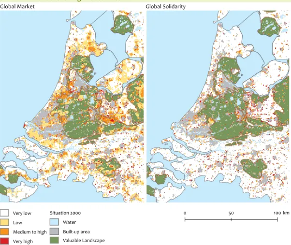
the imagination and broaden the view on the future. Impor-tant elements are: plausible unexpectedness and informa-tional vividness (Xiang and Clarke, 2003). An example of such a scenario-based simulation of land-use change is offered by (Borsboom-van Beurden et al., 2007; Borsboom-van Beurden et al., 2005). This analysis was performed to evaluate the possible impact on nature and landscape in scenarios on the future, as described in the first national sustainability outlook (MNP, 2004). The qualitative storylines of the original scenario framework were translated in spatially explicit assumptions, regarding the locational preferences and future demand of a large number of land-use types, by means of expert workshops and sector specific regional models. The results of the study were subsequently used to inform the National Parliament. The general public was also informed through, for example, publicity in the national media (Schreuder, 2005). This study pointed out that increased land use by housing, employment and leisure, will contribute to further urbanisation, especially in the centre of the Neth-erlands. This will result in deterioration of nature areas and valuable landscapes, depending upon the degree of govern-ment protection assumed in a scenario (Figure 1.2). Another recent application at the national level simulated future land-use patterns according to two trend-based scenarios and

subsequently optimised the projected spatial developments according to specific planning objectives to show possible alternative land-use configurations that may result from policy interventions (MNP, 2007).

The above mentioned applications have in common that they follow a what-if approach; they indicate what may happen if certain conditions occur. This implies that the main task of the applied land-use model is not so much to create the most probable, future land-use pattern, but rather to produce out-comes that match the envisioned future conditions.

Report layout

1.2

The present report is organised as follows. The following section will further introduce the Land Use Scanner. Here, the model basics and its two available allocation algorithms are briefly discussed, and previous calibration efforts are mentioned. Section 3 proceeds to present the methodology applied in this report. The Sections 4 and 5 then describe the actual calibration and validation of the Land Use Scanner. The final section lists the plans for further research.

Land use simulated according to the A1 (left) and B1 (right) scenarios: the intensity of the red colour indicates a possible increase in urban pressure, the green areas inside the grey contours signify valuable landscapes (Borsboom-van Beurden et al., 2005).

Figure 1.2 Simulated land use following two scenarios

Very low Low Medium to high Very high Situation 2000 Water Built-up area Valuable Landscape Global Market 0 50 100km Global Solidarity

(14)

(15)

Land Use Scanner 15

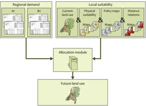
The Land Use Scanner is a GIS-based model that produces simulations of future land use, based on the integration of sector-specific inputs from dedicated models. The model is based on demand-supply interaction for land, with sectors competing for allocation within suitability and policy con-straints. It uses a comparatively static approach that simu-lates a future state, in a limited number of time steps. Recent applications simulate land-use patterns in three subsequent time steps (MNP, 2007), whereas initial applications used only one or two. Unlike many other land-use models, the objective of the Land Use Scanner is not to forecast the dimension of land-use change, but rather to integrate and allocate future land-use demand from different sector-specific models or experts. This is depicted in Figure 2.1, presenting the basic structure of the Land Use Scanner.

External regional projections of land-use change, which are usually referred to as demands or claims, are used as input for the model. These are land-use type specific and can be derived from, for example, sector-specific models of special-ised institutes. The predicted land-use changes are considered

as an additional demand for the different land-use types, compared with the present area in use, for each land-use type. The total of the additional demand and the present area for each type of land use is allocated to individual grid-cells, based on the suitability of the cell. This definition of local suit-ability may incorporate a large number of spatial data sets, referring to the following aspects that are discussed below: current land use, physical properties, operative policies and market forces, generally expressed in distances related to nearby land uses.

Current land use offers the starting point in the simulation of future land use. Therefore, it is an important ingredient in the specification of both the regional demand and the local suitability. Current land-use patterns are, however, not necessarily preserved in model simulations. This offers the advantage of having a large degree of freedom in generating future simulations, according to scenario specifications, but calls for attention when current land-use patterns are likely to be preserved.

Land Use Scanner

2

Basic layout of the Land Use Scanner.

Figure 2.1 Land Use Scanner

Regional demand

Allocation module

Future land use

Local suitability

Current land use

&

Physical

suitability Policy maps Distancerelations

A1 B2 Maps 1 2 N Maps 1 2 N Maps 11 2 N

(16)

The physical properties of the land (e.g. soil type and ground-water level) are especially important for the suitability specification of agricultural land-use types as they directly influence possible yields. They are generally considered to be less important to urban purposes, as the Netherlands have a long tradition of manipulating their natural conditions. However, operative policies help steer Dutch land-use develop-ments in many ways, and are important components in the definition of suitability. The national nature development zones and the municipal urbanisation plans are examples of spatial policies that stimulate the allocation of certain types of land use. Restrictions are offered by various zoning laws related to, for example, water management and the preserva-tion of landscape values.

The market forces that steer residential and commercial devel-opment, for instance, are generally expressed in distance relations. Especially the proximity to railway stations, highway exits and airports, are considered important factors that reflect the locational preferences of the actors, which are active in urban development. Other factors that reflect such preferences are, for example, the number of urban facilities or the attractiveness of the surrounding landscape. The selection of the appropriate factors for each of these components and their relative weighing, are crucial steps in the definition of the suitability maps and largely determine the simulation outcomes. The relative weights of the factors, which describe the market forces and operative policies, are normally assigned in such a way that they reflect the scenario storylines. Obviously, these scenario-related suitability defini-tions cannot be validated, as they essentially reflect the imagi-nation of the modeller. Instead, the current calibration effort is mainly aimed at assessing the performance of the available allocation algorithms. An additional objective, however, is to help pinpoint the most important location factors in the suitability map definition. Furthermore, the relative weighing of the suitability values of the different land-use types will be evaluated, as a recurring issue in their definition is how to scale the values of, for instance, residential land use in rela-tion to agriculture.

The following sections describe the two allocation algorithms in more detail. The last section briefly discusses previous cali-bration attempts for the Land Use Scanner and summarises several studies which have tried to quantify the importance of various location factors for past land-use changes.

Continuous model

2.1

The original, continuous model employs a logit-type approach, derived from discrete choice theory. Nobel prize winner McFadden has made important contributions to this approach of modelling choices between mutually exclusive alternatives (McFadden, 1978). In this theory, the probability that an individual selects a certain alternative is dependent on the utility of that specific alternative, in relation to the total utility of all alternatives. This probability is, given its defini-tion, expressed as a value between 0 and 1, but it will never

reach these extremes. When translated into land use, this approach explains the probability of a certain type of land use at a certain location, based on the utility of that location for that specific type of use, in relation to the total utility of all possible uses. The utility of a location can be interpreted as its suitability for a certain use. This suitability is a combination of positive and negative factors that approximate benefits and costs. The higher the utility (suitability) for a land-use type, the higher the probability that the cell will be used for that type. Suitability is assessed by potential users and can also be interpreted as a bid price. After all, the user deriving the highest benefit from a location will offer the highest price. Furthermore, the model is constrained by two conditions, namely, the overall demand for each type of land use, and the amount of land which is available. By imposing these conditions, a doubly constrained logit model is established, in which the expected amount of land in cell c that will be used for land-use type j is essentially formulated as:

(1)

in which:

Mcj is the amount of land in cell c expected to be used for

land-use type j;

aj is the demand balancing factor (condition 1) that ensures

that the total amount of allocated land for land-use type j equals the sector-specific claim;

bc is the supply balancing factor (condition 2) that makes

sure the total amount of allocated land in cell c does not exceed the amount of land that is available for that particular cell;

Scj is the suitability of cell c for land-use type j, based on its

physical properties, operative policies and neighbourhood relations. The importance of the suitability value can be set by adjusting a scaling parameter.

The appropriate aj values that meet the demand of all

land-use types, are found in an iterative process, as is also discussed by (Dekkers and Koomen, 2007). This iterative approach, in fact, simulates a bidding process between competing land users (or, more precisely, land-use classes). Each use will try to get its total demand satisfied, but may be outbid by another category that derives higher benefits from the land. Thus, it can be said that the model, in a simplified way, mimics the land market. The government policies that strongly limit the free functioning of the Dutch land market, can be included in this process in the suitability map defini-tion by means of taxes and subsidies. In fact, the simuladefini-tion process produces a kind of shadow price for land within the cells. This is discussed in more detail elsewhere (Koomen and Buurman, 2002).

In reality, the allocation process is more complex than sug-gested in the described basic formulation. The most impor-tant extensions are briefly discussed below:

The location of a selected number of land-use types –

(infrastructure, water, exterior) is fixed in the model

cj

(17)

Land Use Scanner 17

and anticipated developments (e.g. the construction of a new railroad) are supplied exogenously to the simulations;

The land-use claims are specified per region and this –

regional division may differ per land-use type, thus creat-ing a complex set of demand constraints;

Minimum and maximum claims are introduced to make –

sure that the model has a feasible solution. For land-use types with a minimum claim it is possible to allocate more land. With a maximum claim it is possible to allo-cate less land. The latter type of claim is essential when the total of all land-use claims exceeds the available amount of land;

To reflect the fact that urban land users, in general, will –

outbid other users at locations that are equally well suited for either type of land use, a monetary scaling of the suitability maps has recently been introduced (Borsboom-van Beurden et al., 2005; Groen et al., 2004). In this approach, the maximum suitability value per land-use type is related to a realistic land price, ranging from, for example, 2.5 €/m2 _{for nature areas to 35 €/m}2 _for

resi-dential areas. The merits of this approach are currently under study by others (Dekkers, 2005).

A more extensive mathematical description of the model and its extensions is provided in a previous paper (Hilferink and Rietveld, 1999).

The continuous model directly translates the probability that a cell will be used for a certain land-use type on a certain amount of land. Thus, a probability of 0.9, in the case of a 100-metre grid, will result in 0.9 ha. This straightforward approach is easy to implement and interpret, but has the disadvantage of potentially providing very small surface areas for many different land-use types in a cell. This will occur, especially, when the suitability maps have little spatial differentiation. A possible solution for this issue is the inclusion of a thresh-old value in the translation of probabilities in surface areas. Allocation can then be limited to those land-use types that, for example, have a probability of 0.2 or higher. The inclu-sion of such a threshold value calls for an adjustment of the allocation algorithm, to make sure that all land-use claims are met. This is feasible, nevertheless, and has been applied in the Natuurplangenerator (Eupen and Nieuwenhuizen, 2002), which — in many ways — is similar to the Land Use Scanner. The experience with this minimal probability teaches that insignificant quantities of land use will be set to zero and, if this threshold value is raised, the model will have difficulty finding an optimum. This is caused by the possibility that all probabilities are below the threshold value. Because of these disadvantages it is not recommended to raise the threshold value.

For visualisation purposes the simulation outcomes are normally aggregated and simplified in such a way, that each cell portrays the single dominant category from a number of major categories. This simplification has, however, substantial influence on the apparent results and may lead to a serious over-representation of some categories and an under-repre-sentation of others. To prevent the above mentioned issues related to the translation and visualisation of the probability

related outcomes, an allocation algorithm was introduced that deals with homogenous cells, as is discussed below.

Discrete model

2.2

The discrete allocation model allocates equal units of land (cells) to those land-use types that have the highest suitabil-ity, taking into account the regional land-use demand. This discrete allocation problem is solved through a form of linear programming. The solution of which is considered optimal when the sum of all suitability values corresponding to the allocated land use is maximal.

This allocation is subject to the following constraints: the amount of land allocated to a cell cannot be –

negative;

in total only 1 hectare can be allocated to a cell; –

the total amount of land allocated to a specific land-use –

type in a region should be between the minimum and maximum claim for that region.

Mathematically, we can formulate the allocation problem as:

(2)

subject to:

for each c and j; for each c;

for each j and r for which claims are specified;

in which:

Xcjis the amount of land allocated to cell c to be used for

land-use type j;

Scj is the suitability of cell c for land-use type j;

Ljr is the minimum claim for land-use type j in region r; and

Hjris the maximum claim for land-use type j in region r.

The regions for which the claims are specified may partially overlap, but for each land-use type j, a grid cell c can only be related to one pair of minimum and maximum claims. Since all of these constraints relate Xcj to one minimum claim, one maximum claim (which cannot both be binding) and one grid cell with a capacity of 1 hectare, it follows that if all minimum and maximum claims are integers and feasible solutions exist, the set of optimal solutions is not empty and cornered by basic solutions in which each Xcj is either 0 or 1 hectare. The problem at hand is comparable to the well-known Hitchcock transportation problem that is common in transport−cost minimisation and, more specifically, the semi-assignment problem (Schrijver, 2003; Volgenant, 1996). The

max_X

S

_cj

X

_cj cj

∑

Xcj≥0 Xcj j

∑

=1 Ljr≤ Xcj c

∑

≤H_jr

(18)

objective here is to find the optimal distribution, in terms of minimised distribution costs of units of different homogenous goods, from a set of origins to a set of destinations under the constraints of a limited supply of goods, a fixed demand, and fixed transportation costs per unit for each origin−destination pair. The semi-assignment problem has the additional charac-teristic that all origin capacities are integer and the demand of each destination is one unit. Both are special cases of linear programming problems. The discrete allocation algorithm has two additional characteristics, which are not incorporated in the classical semi-assignment problem formulation: (1) we can specify several, (partially) overlapping regions for the claims (although the regions of claims for the same land-use type must be disjoint); and (2) it is possible to apply distinct minimum and maximum claims.

Our problem, with its very large number of variables, calls for a specific, efficient algorithm. To improve the efficiency, we apply a scaling procedure and also use a threshold value. Scaling means that we use growing samples of cells in an iterative optimisation process that has proven to be fast (Tokuyama and Nakano, 1995). For each sample an optimi-sation is performed. After each optimioptimi-sation, the sample is enlarged and the shadow prices in the optimisation process are updated in such way that the (downscaled) regional con-straints remain respected. To limit the number of alternatives under consideration we use a threshold value: only allocation choices that are potentially optimal are placed in the priority queues for each competing claim. An important advantage of the applied algorithm is that we are able to find an exact solution using a desktop PC (Pentium IV-2.8 GHz, 1 GB internal memory), within several minutes, provided that feasible solu-tions exist and all suitability maps have been prepared in an initial model run. Running the model for the first time takes just over an hour, as all base data layers have to be con-structed. These data sets are then stored in the application files (in a temporary folder) to speed up further calculations. The constraints that are applied in the new discrete allocation model are equal to the demand and supply balancing factors applied in the original, continuous version of the model. In fact, all the extensions to the original model related to the fixed location of certain land-use types, the use of regional claims, the incorporation of minimum/maximum claims and the monetary scaling of the suitability maps, also apply to the discrete model. Similar to the original model, the applied opti-misation algorithm aims to find shadow prices for the regional demand constraints that increase or decrease the suitability values, such that the allocation based on the adjusted suit-ability values corresponds to the regional claims. The main difference of the discrete model is that each cell only has one land-use type allocated, meaning that for each land-use type the share of occupation is zero or one. However, from a theoretical perspective the models are equivalent when the scaling parameter that defines the importance of the suit-ability values would become infinitely large. In the latter case, the continuous model would also strictly follow the suitability definition in the allocation and produce homogenous cells. This procedure, however, is theoretical and cannot be applied in the calculations due to computational limitations.

Previous calibration efforts

2.3

Many different model components of the original, continu-ous land-use model, have received ample research attention over the past 10 years. Initial calibration efforts focused on the appropriate number of iterations and estimation of the β-parameter (Hilferink and Rietveld, 1999). Subsequent efforts analysed the development of the shadow prices and concluded that the model neatly converged to equilibrium prices, when the minimum and maximum claims were used in such a way that a feasible solution existed (Ransijn et al., 2001).

A first attempt to calibrate the suitability maps for individual land-use types, was done for single and multi-family dwellings (Rietveld and Wagtendonk, 2004; Wagtendonk and Rietveld, 2000). The main factors influencing the location of new residential areas were analysed, in the period from 1980 to 1995, by means of binomial logistic regression. They claim the most significant variables to be: ‘the proximity of a location to existing residential areas; location in new towns, receiving government support; the accessibility of workplaces; distance to railway stations; and, to a lesser extent, the accessibility of nature, surface water, and recreational areas’. These findings have been applied in a simulation of new residential develop-ment in the 1995 to 2020 period (Schotten et al., 2001b). A further attempt at calibrating the suitability maps in the Land Use Scanner, was focussed on commercial land use (Wagtendonk and Schotten, 2000). The analysis of the loca-tion factors, which contributed to the growth of commercial areas (trade, industry and services) in the 1981 to 1993 period, proved the importance of whether a location was situated in the city centre or at the outskirts, and also quantified the impact of the distance to railway stations and highway exits. These results were used in Land Use Scanner simulations of commercial land use in 1993, and were visually compared to the actual commercial land use in that year. This comparison proved the potential of this approach, but also indicated two important drawbacks: (1) regional differences in suitability for specific land uses could not directly be accounted for and (2) historic concentrations, pre-dating the 1981 to 1993 develop-ment, were not explained very well, with this approach. These issues are solved in subsequent Land Use Scanner simulations through the inclusion of regionally defined land-use claims, which take into account the differences in commercial devel-opment per region, and the explicit inclusion of current land use in the description of suitability.

The wealth of general research dedicated to the location factors that influence land-use development, also provides valuable information for the calibration of the Land Use Scanner. Especially relevant in the Dutch context, is the work of (Verburg et al., 2004) where binomial logistic regression was applied to assess ‘the probability of land-use change at a certain location, relative to all other options’. This approach was selected instead of multinomial logistic regression, to be able to use different explanatory factors for the different types of land-use change. The analysis made use of a 500-metre grid, which described a single, dominant land use per cell. This aggregation was based on the majority rule, but a

(19)

Land Use Scanner 19

correction was applied to ensure that the total area for each land use corresponded to the underlying higher resolution base maps. The analysis explained the observed 1989 land use, from a series of location characteristics that were con-sidered relevant for the historic development of the Dutch landscape. These characteristics consisted of the biogeophysi-cal conditions (soil type and altitude), the distance to open water (coast and main rivers) and the distance to historic town centres. This set of explanatory variables worked well to explain the location of agriculture and nature. Urban develop-ment could not be easily explained, possibly indicating the importance of non-spatial self-organising processes, and the difficulty to represent the temporal dynamics of land-use change in a static analysis. The latter part of the analysis, therefore, focused on the major short-term land-use changes observed in the 1989 to 1996 period, being the development of new residential, industrial/commercial and recreation areas. These changes were no longer related to biophysical properties, but rather to spatial policies, accessibility and neighbourhood interactions. The most important location factors, which were distinguished in the study of Verburg and others, are normally also included in the suitability maps of the Land Use Scanner.

A major disadvantage of the studies described above, is that they tend to focus on the probability of occurrence of single land-use types. None of the studies examine this probability in relation to the probability of occurrence of the other land-use types, as is the topic of the present study.

An initial integrated validation of the Land Use Scanner was performed as part of an extensive comparison of several contemporary land-use change models (Pontius Jr. et al., 2008). The validation followed a straightforward, quantita-tive approach, in which a map with observed land use of the initial year is compared to maps with observed and predicted land use of a subsequent year. This set of maps allows for the comparison between actual change and predicted change and, furthermore, assesses the performance of the model in relation to a null model of persistence. The latter indi-cates whether the model performs better than a no-change approach. These comparisons are performed at multiple resolutions, to analyse whether the observed inaccuracy can be attributed to relatively small locational errors. For the Land Use Scanner this analysis was performed on an adjusted scenario-based simulation of the year 2000, based on 1996 maps, without a preceding calibration effort. The amount of land-use change per land-use type (claims) was derived from a 1981 to 1996 trend analysis. First and foremost, the exercise showed the strong impact of the reformatting of the original, heterogeneous output maps, to the homogenous, maps of dominant land-use needed for the validation. The inaccuracy introduced by the reformatting turned out to be larger than the actual change in the short observation period. Other issues that hamper this validation, are the inconsistencies in the base maps of observed land use, obscuring the actual land-use changes. The reformatting issue does not apply to the present validation analysis, because a different method is presented for comparing the simulation results of the continuous model (see the discussion on map comparison in Section 3). The issue is absent in the presented analysis of the

discrete model, because discrete maps of both current and simulated land use are being used. In the actual land-use simu-lations, however, a similar issue may occur when the discrete simulation starts from a base map that uses a heterogeneous, continuous description of land use per cell. Therefore, we recommend that upcoming simulations start from a data set which uses a discrete specification of current land use.

(20)

(21)

Methodology 21

To assess the potential of the new fine resolution in produc-ing sensible land-use patterns and to compare the perform-ance of the two available algorithms, a two-step approach is used that first calibrates the model and then validates the simulation results for a subsequent time step, for which a reference data set with observed land use is available. This strict distinction between the calibration and validation phase means that only information available at the initial calibra-tion time step is used to tune the model. This is advocated in literature (Pontius Jr. et al., 2004) and means that we are able to properly assess the predictive power of the model. In the calibration step the model’s suitability maps are tuned, based on a statistical analysis of the observed land-use patterns of 1993. The obtained relations are then used to simulate land use in 2000. A pixel-by-pixel comparison between the simu-lated and the observed land use of 1993 and 2000, reveals the performance of the model. This section describes the most important elements in the applied methodology: the incorpo-rated land-use data sets, the statistical regression analysis and the applied map comparison methods.

The analysis is performed on the two available 100-metre models. This choice is motivated by our special interest in assessing the potential of the new fine resolution, and comparing the performance of the two available allocation algorithms. For computational reasons we use a simplified model configuration that simulates five major types of land use and uses only one time step in the simulation process. For the calibration and validation we use the exact amounts of land per type for 1993 and 2000, respectively. The analysis, thus, focuses solely on the simulated land-use patterns and not on the amount of land-use change. This distinction is common in map comparison research (e.g. Pontius Jr., 2000) and, in our case, means that we only assess the functioning of the allocation algorithms and the impact of the suitability defi-nitions and not of the procedures that are normally used for obtaining future land-use demand. As the latter information is normally derived from external sources, we do not consider this a major drawback in the scope of the current calibration and validation analysis (for additional validation aspects, see Chapter 6).

Land-use data

3.1

Starting point in this calibration effort is the 1993 land use, based on the spatial land-use data set of the Central Bureau

for Statistics (CBS, 1997). This data set, with 34 classes, has been reclassified in nine major types of land use: agriculture, nature, commercial areas, residential areas, recreation, infrastructure, other, water, exterior. The first five land-use types are simulated by the model. The remaining land-use types have a pre-defined location, which is not influenced by model-simulation. This limited set of land-use types has several advantages; it provides a clear insight in the alloca-tion process, it is relevant in policy evaluaalloca-tion studies, and it allows the use of a standard package for subsequent statisti-cal analyses.

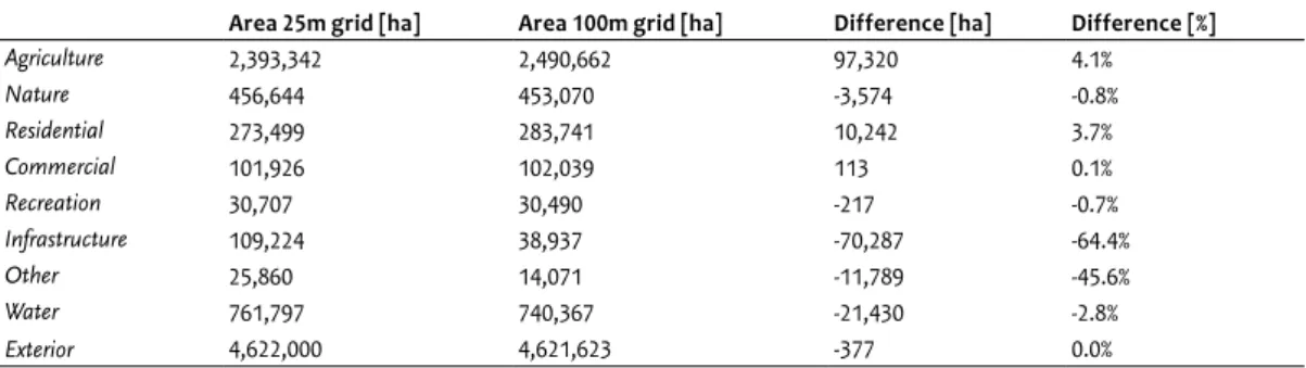
To apply the original 25-metre grid land-use data set in the Land Use Scanner that uses a 100-metre resolution, the data were also aggregated to this coarser resolution by using the majority rule. This aggregation leads to an over repre-sentation of the land-use types that structurally claim most (agricultural and residential land), but not all of the constitut-ing grid cells. Under-representation of certain land-use types occurs when these, in general cover only a small part of the aggregated cells. Table 3.1 shows that especially the impact of under-representation is considerable for infrastructure and the remaining land-use type ‘other’. This does not pose a major problem to our simulations as the location of these land-use types are supplied exogenously to the model. The aggregation impact for the land-use types that are actually simulated in the model is considered to be of minor impor-tance as their total area in the 100-metre grid does not differ more than 4% from the original 25-metre grid.

A major disadvantage of the available land-use data sets is that they are not methodologically consistent through time. A number of unlikely conversions become apparent, when a pixel-by-pixel transition matrix is created. Table 2 sum-marises the results of this analysis. The conversion of about 13,000 ha of residential areas and 10,000 ha of infrastructure into agriculture, for example, is highly unlikely in the Nether-lands, which are characterised by a continuously increasing degree of urbanisation. These conversions are related to changes in the data collection and classification methods (CBS, 1997; CBS, 2002; Raziei and Evers, 2001). Through the changed methodology, unpaved and partially paved roads, the shoulders of paved roads and railroads, for example, have been reclassified according to the surrounding land uses (mainly agriculture and nature). The observed conversion of residential land into agricultural land mainly refers to sparsely built-up areas, in elongated rural villages and other hamlets

(22)

that are considered not to be fully built-up anymore, in the new classification method.

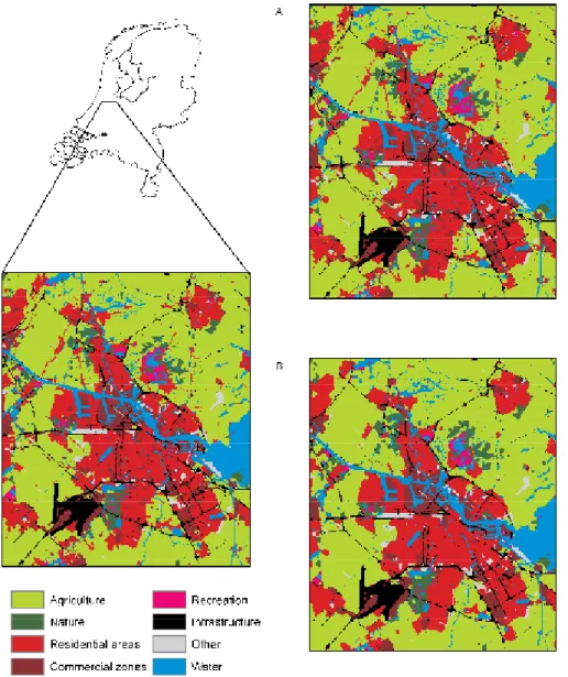
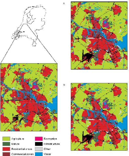
In fact, many of the changes in Table 3.2 have to be viewed with caution. This is especially true for the loss of infrastruc-ture, as was discussed above, the loss of water and the local increase in agricultural areas. Discarding the changes in the exterior that were partly introduced in the subsequent data treatment process, these suspicious changes apply to over 60,000 hectares. This is equivalent to almost 36% of all observed changes other than those in the exterior. Not all of these observed changes are necessarily erroneous, but many of them are likely to be related to phenomena, such as: changes in the classification methodology; changes in the per-ception of the data collector (for example, when agricultural areas also have natural or recreational values), differences in the water levels at the time of observation (that may account for local gain or loss of water filled areas) or locational mis-matches between the different data sets (that may suggest wandering land-use objects). It is evident, that such methodo-logical inconsistencies strongly hamper the analysis of actual changes. The inconsistencies also present a major difficulty in assessing the performance of a land-use simulation, as it is dif-ficult to distinguish between actual and apparent changes. Figure 3.1 shows the land-use data sets and their major differ-ences, for an area around Amsterdam. The difference map presents the two most common conversions: the conversion of agricultural land into residential areas and into nature. It is clear that most transitions occur in large, contiguous areas, which are normally adjacent to existing residential or natural areas. A comparison of the land use in 1993 and 2000 also

indicates where infrastructure has disappeared, since 1993. This is mainly the case for secondary roads, which are repre-sented as smaller areas leading to an increase in the adja-cent, agricultural land use in 2000. The large infrastructural complex (Schiphol airport) is also represented by a smaller area in 2000, again leading to an increase in agriculture. These unwanted conversions are corrected, by excluding the 1993 infrastructural locations from the calibration and validation. In fact, all locations with an exogenous land-use type, in either 1993 or 2000, are excluded in the subsequent calibration and validation exercises.

Regression analysis

3.2

Different sets of statistical relations that describe the land-use configuration in 1993 are established by using multinomial logistic regression (MNL) analysis. This method of regression is useful in situations where categories in a dependent vari-able, based on values of a set of independent variables, have to be predicted. The method is similar to binomial logistic regression, but the dependent variable is not restricted to two categories. The main advantage of MNL regression is the possibility of estimating the relative probabilities for each category in the dependent variable, with a set of inter-related logistic equations. This is an advantage compared to the alternative approach of using a set of separate binomial logistic regressions that would not estimate these probabili-ties relative to each other. The dependent variable has to be categorical and, in this case, it relates to the five types of land use that are used in the simulation. Agriculture is used as a reference category in the analysis, meaning that all probabili-Total area covered by main land-use types in 1993 for the 25-metre base grid and the aggregated 100-metre grid

Area 25m grid [ha] Area 100m grid [ha] Difference [ha] Difference [%]

Agriculture 2,393,342 2,490,662 97,320 4.1% Nature 456,644 453,070 -3,574 -0.8% Residential 273,499 283,741 10,242 3.7% Commercial 101,926 102,039 113 0.1% Recreation 30,707 30,490 -217 -0.7% Infrastructure 109,224 38,937 -70,287 -64.4% Other 25,860 14,071 -11,789 -45.6% Water 761,797 740,367 -21,430 -2.8% Exterior 4,622,000 4,621,623 -377 0.0% Table 3.1

Matrix of transitions in observed dominant land use at a 100-metre resolution

1993

2000 Agriculture Nature Residential Commercial Recreation Infra. Other Water Exterior Total 2000

Agriculture 2425550 7751 12968 2759 976 10232 2344 2223 132 2464935 Nature 23606 435958 2441 2599 3212 2524 778 1543 38 472699 Residential 24597 3660 258971 12221 835 2667 6320 725 8 310004 Commercial 6003 879 6768 76782 164 1127 244 444 5 92416 Recreation 2112 1094 448 488 23503 167 96 282 4 28194 Infra. 2952 719 864 1064 82 21475 251 239 0 27646 Other 2108 294 336 2495 49 205 3726 274 3 9490 Water 3638 2700 918 3628 1668 538 311 734629 291027 1039057 Exterior 96 15 27 3 1 2 1 8 4330406 4330559 Total 1993 2490662 453070 283741 102039 30490 38937 14071 740367 4621623 8775000

Note: the figures denote hectares, the retention frequencies are shaded grey.

(23)

Methodology 23

ties are estimated relative to this category. The independent variables in the analysis can be factors or co-variants and, in our case, relate to the surrounding land use, the proximity of infrastructure and specific policy maps.

Applied to the statistical analysis of land-use patterns, the selected approach explains the probability of a certain type of land use at a certain location, based on the utility of that loca-tion for that specific type of use, in relaloca-tion to the total utility of all possible uses. The utility of a location can be interpreted as its suitability for a certain use, and is described with several geographical data sets, which represent location factors. This can be formulated as follows:

cj

P

=

e

β ∗Xcj

e

β ∗Xck

k

∑

(3)

Where:

Pcj is the probability for cell c being used for land-use type j;

e is the basis for the natural logarithm;

ß is a vector of estimation parameters for all variables x; Xcj is a set of location factors (explanatory variables) for cell c

for land-use type j; and

Xck is a set of location factors for cell c for all (k) land-use

types.

This logit specification is identical to the original, continu-ous allocation model and, thus, allows for a straightforward inclusion of the estimated coefficients in the suitability maps of the Land Use Scanner. The suitability value of the reference category is 0 in all locations, but since the other suitabilities are estimated relative to this value, it is still possible to also

Comparison of the observed 1993 and 2000 land use.

Figure 3.1

(24)

simulate agricultural land use with the model. In fact, using another reference category would yield different coefficients but produce an identical land-use map after simulation.

Selection of independent variables 3.2.1

Most of the selected independent variables in the multinomial logistic regression analysis are related to the surrounding land-use types, as these are known to greatly influence land use at a certain location (Verburg et al., 2004). A total of 27 variables were initially distinguished to describe the land use in three sets of rings surrounding any given cell. These rings contain the 8 immediately neighbouring cells (ring 1), the following 40 cells (rings 2-3), and the subsequent 312 cells (rings 4-9), see Figure 3.2. For each of these three sets of rings, the total number of cells that belong to each of the nine distinguished land-use types is expressed as an integer value, ranging from 0 to 8. For ring 1 this integer corresponds exactly with the observed number of cells; for the combina-tion of rings 2 and 3, this integer is the rounded value of the total number of cells dived by 5 and 39, respectively. This so-called autologistic specification estimates the probability that a certain land use occurs, as a function of the total number of cells that belong to each of the nine distinguished land-use types. Implementation of the suitability values that are, thus, derived causes the model to perform in a neighbourhood-oriented manner that is similar to classical Cellular Automata. In addition to the above autologistic specification, a number of location characteristics were also added. These extra inde-pendent variables relate to two types of driving forces that are considered important in land-use development: accessibil-ity (distance to stations and presence of railways and main roads) and spatial policies (related to nature development and nature preservation policies). Table 3.3 presents a short overview of the additional variables. The impact of other spatial variables related to the presence of, for example, underground infrastructure, power lines, soil subsidence, motorway exits, airport noise contours and the borders of the Green Heart (the central open space surrounded by the rim of major Dutch cities known as the Randstad), was tested in initial model specifications, but did not yield statistically sig-nificant results. Inclusion of a more extensive set of variables is, however, considered for future research.

3.2.2 Estimation results

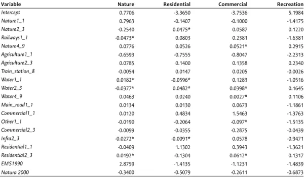
The statistical analysis was performed with the standard soft-ware package SPSS (version 13) using 19 different explanatory variables, 14 of which describe the presence of a land-use type in one of the three sets of rings surrounding the cell. The remaining five variables refer to accessibility and spatial

poli-cies. The coefficients resulting from the regression analysis are presented in Table 3.4. The statistical model performs quite well, explaining about 90% of the variance (pseudo R2

Nagelkerke of 0.90).

The suitability of a cell for a certain land-use type, in most cases, is positively correlated with the occurrence of the same land-use type in its immediate surroundings. The suitability for nature, for example, increases with 0.77 for every nature cell in the first ring (denoted in the table with Nature1_1). A nega-tive correlation is observed for the probability of nature, with the presence of residential land in the first ring. The opposite is true for the relation with the land use in the second and third ring. Here, identical land uses seem to repel rather than attract each other. The probability of residential land, for example, decreases slightly with the presence of residences in ring 2 and 3, yet it increases a little with the presence of agricultural land use. These unexpected relations may be interpreted as small corrections for the strong correlation with these land-use types in ring 1. The estimate for recrea-tion differs considerably from the other types of land use, in the sense that neighbouring recreational land use did not produce a significant result. This may be caused by the limited number of recreation observations and by the fact that recreation occurs in smaller spatial clusters. Please note that 11 of the total of 27 possible variables, related to neighbouring land-use types, are not included in the presented regression results, as they did not produce statistically significant results. The suitability values of the reference category (agriculture) were set to zero.

Map Comparison

3.3

To compare the maps of the different model runs, simple cell-to-cell comparisons of simulated and observed land use are used, in either 1993 (calibration) or 2000 (validation). These comparisons are made for all simulated land-use types sepa-rately, to individually assess their performance. An overall degree of correspondence for the whole simulation has not been calculated, as this would be largely equal to the value of the prevailing land-use type (agriculture). The selected, straightforward comparison approach is easy to comprehend and very informative. Other, more complex comparison methods that deliver, for example, (Fuzzy)Kappa statistics or log-likelihood values (De Pinto and Nelson, 2006; Hagen, 2003; Munroe and Muller, 2007; Pontius Jr. et al., 2004; Visser and De Nijs, 2006), are more difficult to interpret and, therefore, have not been applied. Application of a comparison method that looks beyond single cells and includes corre-Overview of the non-neighbourhood related independent variables in the Multinomial regression

Independent variable Explanation

Railways1_1 Buffer of 100 metres around the railways (derived from the

origi-nal land-use file from Statistics Netherlands, CBS, 1997)

Train_station_8 distance to nearest train station indicated as an index

val-ue between 1 and 8 (derived from: AVV, 1994)

Main_road1_1 Buffer of 100 metres around main roads (derived from the

origi-nal land-use file from the Statistics Netherlands, CBS, 1997)

EMS1990 Ecological Main Structure, Designated areas for nature areas of high quality (RIVM et al., 1997)

Natura 2000 European network of protected nature areas (IKC-Natuurbeheer, 1993)

(25)

Methodology 25

spondence in neighbouring cells (such as the FuzzyKappa sta-tistic) is likely to produce better results. We do not consider this appropriate in our case, however, as we explicitly include

reference to the current state of the neighbouring cells in the suitability map definition. Calculating a degree of cor-respondence that would incorporate this information would,

The three sets of rings (1, 2-3 and 4-9) surrounding the central observation point, which are used as explanatory variables in the multinomial logistic regression.

Figure 3.2

Surrounding land use as explanatory variables

Estimated coefficients of the Multinomial logit model

Variable Nature Residential Commercial Recreation

Intercept 0.7706 -3.3650 -3.7536 5.1984 Nature1_1 0.7963 -0.1407 -0.1000 -1.4175 Nature2_3 -0.2540 0.0475* 0.0587 0.1220 Railways1_1 -0.0473* 0.0803 0.2381 -1.6381 Nature4_9 0.0776 0.0526 0.0521* 0.2915 Agriculture1_1 -0.6593 -0.7555 -0.8047 -2.2313 Agriculture2_3 0.0785 0.1400 0.1358 0.2340 Train_station_8 -0.0054 0.0147 0.0205 -0.0026 Water1_1 0.0182* -0.0596* 0.1283 -1.0516 Water2_3 -0.0377* 0.0482* 0.0398* 0.1645 Water4_9 0.0463 0.0240 0.0027* 0.1106 Main_road1_1 0.0134 0.0130 0.0673 -1.1861 Commercial1_1 0.0120 0.4834 1.5463 -1.3763 Other1_1 -0.0190 -0.2064 -0.097* -1.5135 Commercial2_3 -0.0099 -0.0355 -0.2875 -0.0439 Infra2_3 -0.0272* -0.0091* 0.0578 -0.9471 Residential1_1 -0.0409 1.1302 0.3943 -1.3621 Residential2_3 0.0192* -0.1304 0.0612* 0.1317 EMS1990 2.8759 -1.4135 -1.1231 -1.4839 Natura 2000 -0.3400 -0.5079 -0.2611 -0.6873

Note: all variables are significant at the 0.05 level unless indicated with an asterisk.

(26)

thus, artificially increase the observed match and, moreover, obscure the exact performance of the model.

For the discrete model that contains homogenous cells the share of simulated cells that corresponds to the observed land use is calculated per land-use type. While interpreting these values, it is important to note that the observed land use is not necessarily true or correct, as was discussed previ-ously in Section 3.1 For the continuous model, two methods were used to compare the maps. One is identical to the method used to compare the discrete maps, and compares the dominant land use of the result map with the original map of dominant land-use. The other method is slightly more complex and compares the ratios of simulated and observed land use per cell as follows:

j

C

= cj

M

−

O

_cj 2 c

∑

cj

O

c

∑

(4) where:

Cjis the degree of correspondence for land-use type j;

Mcj is the simulated amount of land in cell c for land-use type j;

Ocj is the observed amount of land in cell c for land-use type j.

In this case, observed land use is also described as a fraction, based on an aggregation of the 16 original grid cells from the 25-metre grid base map that comprise the 100-metre grids. Subsequently, all these differences are added up and this total allocation difference is used to calculate the share of correspondence as part of the total allocated area. Because the exact (observed) quantities of land use have been used in the calibration and validation, the surplus of allocated land in one cell corresponds with a deficit in other cells. This implies, of course, that the total of all differences equals zero and, therefore, the absolute values of these differences are to be summed. As a result, single allocation differences are considered twice and, therefore, we divide the total of the observed errors by two. The resulting share of correspond-ence equals 100% when the amount of allocated land is equal to the observed amount in every cell. Conversely, the share equals zero when none of the allocated amount of land is present in the corresponding cells with observed land use. If we would have considered all allocation differences here without dividing them by two, the share of correspondence could theoretically range from 100% to -100%. The applied com-parison method has the additional advantage of producing a degree of correspondence that is fairly comparable to the one calculated for the discrete model. In fact, the method would produce identical results when the continuous model would only simulate fractions of 0% or 100% per cell.

The so-called exogenous land-use types whose locations are fixed by the model (water, infrastructure and exterior) are not included in the calibration and validation of the model. The main reason for this is that calibrating these land-use types is futile as the model does not attempt to simulate

their dynamics. Including these land-use types would, in fact, provide an overly positive impression of the performance of the model, as these types of land use are extremely static and cover 62% of the total model area; simulating no change for these categories, thus, guarantees a strong degree of correspondence between simulated and observed land use. For the present calibration and validation exercise this means that only cells which are completely filled with endogenous land use in 1993, as well as in 2000, have been compared. This has the additional advantage of discarding many of the grid cells where a change in classification methodology suggests changes in observed land use that did not actually occur. This refers, in particular, to those locations that were classified as infrastructure in 1993 and as something else in 2000, as was discussed in Section 3.1 The rare occasions were exogenous land has indeed changed (e.g. infrastructural developments or water reclamation) are, thus, excluded from the analysis. However, in actual model applications, such changes are supplied exogenously to the simulation following existing plans. This, generally, relates to infrastructure development schemes that are typically planned many years before their actual realisation. Therefore, these are relatively easy to incor-porate in simulations of future land use.