A simulation study on the effectiveness of investing effort in corrective actions to improve the project outcome

(1)

A SIMULATION STUDY ON THE

EFFECTIVENESS

OF

INVESTING

EFFORT IN CORRECTIVE ACTIONS

TO

IMPROVE

THE

PROJECT

OUTCOME

Word count: <12.516>

Jan Bonte

01503231

Milan Crombez

01413443

Promotor: Prof. Dr. Mario Vanhoucke

Under the supervision of: Dr. Annelies Martens

Master’s Dissertation submitted to obtain the degree of:

Master in Business Engineering: Operations Management

(2)

I

PERMISSION

We declare that the content of this Master’s Dissertation may be consulted and/or reproduced, provided that the source is referenced.

Jan Bonte, Milan Crombez,

Signature Signature

(3)

II

Foreword

Although we are not professional athletes, we can draw some similarities. Every athlete is inspired by someone or something when starting his career. To conclude our education as Business Engineers in Operations Management, we chose to implement concepts that were central throughout the years. Professor Dr. Vanhoucke introduced us and our fellow students to the key concepts of project management. Intrigued by his enthusiasm and the beauty of project management, we have chosen a research project in this domain. One of the most important lessons we have learned from his course is: “Even when you schedule your project very carefully, things can or will go wrong”. As practical minded persons, we therefore wanted to do research about implementing corrective actions.

Preparation and especially trial and error dominated our last year as students. Health issues in both individual and familiar context did complicate our process. Combining research for a master dissertation with projects in other courses created a challenge. Our motivation, common sense and realism ensured that we handled this process in such way, that we never lost the courage to keep up the good work.

We did imagine spending late evenings at the faculty, scheduling more meetings than time allows us, drinking coffee in order to stay focused and testing the limits of data storage in excel files. This image drastically changed during the last semester. The Belgian government installed at the 13th of March social distancing measures, due to the rise of the Coronavirus, causing serious illness. The board of the University of Ghent reacted on this by closing its facilities for educational purposes, and thus the reality was anything but our imagination. Except for the coffee…

The faculty transformed in our homes. Our desk was our office. The computer devices were more important than they had ever been. But adjusting to a new situation involves some implications that negatively affect the productivity. The meetings on campus were replaced by online video calls and although the advanced informatics allows us to use cameras and to share screens, making it almost a meeting in person, sharing datafiles was much more difficult due to the large amount of data a simulation generates.

Every athlete needs an entourage. First of all, we want to thank our promotor Professor Dr. Vanhoucke for this topic and providing us with the required facilities. Next, Dr. Annelies Martens, our guide throughout this challenge, who provided feedback when we could not see the wood for the trees. Next to her, but not less emphasized, we want to thank our parents and siblings. Not only for the support during the last months, but for the opportunity they gave us to explore and to broaden our knowledge at the University of Ghent. At last, we would like to thank our friends and family. They supported us with advice and feedback.

(4)

III

List of abbreviations

AC Actual Cost

BAC Budget At Completion

BBP Buffered Planned Progress

CI Criticality Index

CMT Central Limit Theory

CPI Cost Performance Indicator

CPM Critical Path Method

CRI Cruciality Index

CV Cost Variance

ES Earned Schedule

E𝐒𝐑 Required

Earned Schedule

EV Earned Value

EVM Earned Value Management

OR-AS Operation Research & Scheduling (research group of Ghent University)

PERT Program Evaluation and Review Technique

PMBOK Project Management Book of Knowledge

PMI Project Management Institute

PV Planned Value

RBCI Relative Buffer Consumption Index

RBMA Relative Buffer Management Approach

RCPS Resource-Constrained Project Scheduling

RSEM Root Squared Error Method

SI Significance Index

SP Serial or Parallel (indicator)

SPC Statistical Process Control

SPI Schedule Performance Indicator

SRA Schedule Risk Analysis

(7)

VI

List of figures

Figure 1: SP indicator ... 3

Figure 2: EVM-metrics ... 6

Figure 3: Required earned schedule (adjusted from Martens, 2017)... 9

Figure 4: Scenarios review periods ... 18

Figure 5.a: Delay reduction by number of crash units (Arbitirary buffer) ... 24

Figure 5.b: Number of projects late (buffer 10%) ... 24

Figure 5.c: Number of projects late (buffer 20%) ... 24

Figure 6.a: Delay reduction by number of crash units (RSEM buffer) ... 26

Figure 6.b: Number of projects late (RSEM buffer) ... 26

Figure 7.a: Delay reduction by timing review periods (Buffer 10%) ... 26

Figure 7.b: Number of projects late (Buffer 10%) ... 26

Figure 7.c: Number of projects crashed (Buffer 10%) ... 26

Figure 8.a: Delay reduction by timing review periods (Buffer 20%) ... 26

Figure 8.c: Number of projects crashed (Buffer 20%) ... 26

Figure 9.a: Delay reduction by timing review periods (RSEM buffer) ... 27

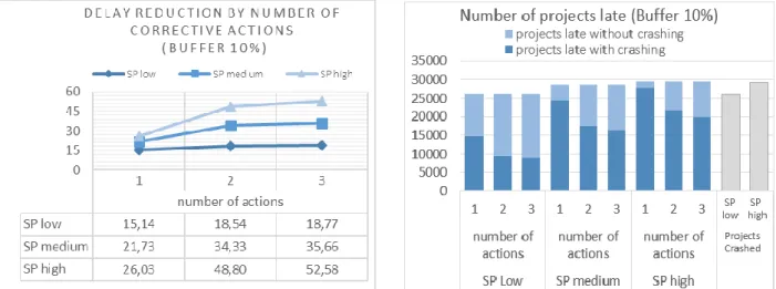
Figure 10.a: Delay reduction by number of corrective actions (Buffer 10%) ... 27

Figure 11.a: Delay reduction by number of corrective actions (Buffer 20%) ... 26

Figure 12.a: Delay reduction by number of corrective actions (RSEM buffer) ... 27

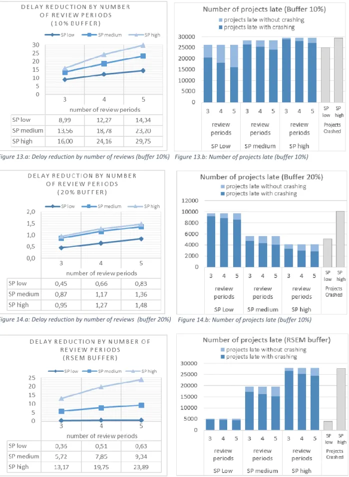
Figure 13.a: Delay reduction by number of review periods (Buffer 10%) ... 30

Figure 14.a: Delay reduction by number of review periods (Buffer 20%) ... 30

Figure 15.a: Delay reduction by number of review periods (RSEM buffer) ... 30

Figure 16.a: Delay reduction by number of actions, late (Buffer 10%) ... 32

Figure 17.a: Delay reduction by number of actions, late (Buffer 20%) ... 32

Figure 18.a: Delay reduction by number of actions, late (RSEM buffer) ... 32

(8)

VII

Figure 19.a: Delay reduction by spreading actions (Buffer 10%, reviews evenly timed) ... 34

Figure 19.b: Delay reduction by spreading actions (Buffer 10%, reviews timed late) ... 34

Figure 19.c: Number of projects late (Buffer 10%)... 34

Figure 20.a: Delay reduction by spreading actions (Buffer 20%, reviews evenly timed) ... 35

Figure 20.b: Delay reduction by spreading actions (Buffer 20%, reviews timed late) ... 35

Figure 20.c: Number of projects late (Buffer 20%)... 35

Figure 21.a: Delay reduction by spreading actions (RSEM buffer, reviews evenly timed) ... 36

Figure 21.b: Delay reduction by spreading actions (RSEM buffer, reviews timed late) ... 36

Figure 21.c: Number of projects late (RSEM buffer) ... 36

Figure 22.a: Delay reduction by crashing percentage (Buffer 10%) ... 38

Figure 23.a: Delay reduction by crashing percentage (Buffer 20%) ... 38

Figure 24.a: Delay reduction by crashing percentage (RSEM buffer) ... 38

(9)

VIII

List of tables

Table 1: Design factors ... 19

Table 2: Efficiency measure (impact number of crash units) ... 23

Table 3: Efficiency measure (impact number of crash units) ... 25

Table 4: Efficiency measure (impact number of corrective actions) ... 29

Table 5: Efficiency measure (impact number of review periods) .. Fout! Bladwijzer niet gedefinieerd. Table 6: Efficiency measure (impact number of actions per period) ... 33

Table 7: Efficiency measure (interaction timing review periods and number of actions) ... 34 Table 8: Efficiency measure (impact crash percentages) ... Fout! Bladwijzer niet gedefinieerd.

(10)

1

Introduction

Many academic researches tackled varying issues in the project management domain. Starting by how to determine the critical path, which buffers to add in order to make the project robust, etc. Project managers come up with a schedule with a planned cost and a planned duration. However, even if estimates are very accurate, things go wrong.

This master dissertation will provide the reader with the answer to the question: what is the impact of

investing effort in activity crashing. We will elaborate this process step by step in this dissertation.

First, we give an overview of the literature that is already published concerning the relevant topics about this research question. The reader will be informed about the different steps of project management, the used techniques for the baseline scheduling, the purpose of Schedule Risk Analysis (SRA) and the different components of project control. Secondly, the research methodology is explained in detail. For predetermined cases, different elements that define crashing effort are tested upon their impact on the project outcome. A simulation study is performed making use of the LUA programming language and the simulation program P2Engine, which is project management and control tool developed by the Operations Research and Scheduling research group of Ghent University. We will pause the projects at predetermined review moments to evaluate its progress and intervene if necessary. These simulations are followed by a statistical analysis is performed for the data generated by the simulation program. In the last section, the results provided by the analysis will be used to answer our research question. In every part, the topics, variables and methods most relevant for our simulation study are explained in detail. In case the reader wishes further information about these concepts, we do advise to take a look at the corresponding references.

(11)

2

Chapter 1: Literature overview

This research topic is situated in the domain of dynamic scheduling. Previous research about this concept was introduced by Uyttewaal (2005) and further explored by Vanhoucke (2012). Three topics are closely linked to this domain: baseline scheduling, schedule risk analysis and project control. The research question about corrective actions is part of the last concept: project control. However, the corrective actions are only necessary when we first perform a control procedure that sets goals which can be achieved using corrective actions. We will evaluate the project at predetermined moments to analyse its performance. Given that project scheduling already incorporates a certain amount of risk, intervention during the simulation is only needed when the goals do not seem to be accomplished.

1.1 Baseline scheduling

1.1.1 Project network

Many research groups came up with various methods to construct the project schedule. The key concepts are elaborated in the Project Management Body of knowledge, PMBOK (2004). Herroelen & Leus (2001) and Herroelen & Demeulemeester (2002) investigated exact solution procedures, Vanhoucke (2012) provides a clear overview of the different techniques to schedule activities. We distinguish the critical path method (CPM), the program evaluation and research technique (PERT) and the resource-constrained project scheduling (RCPS). The PERT/CPM searches the bottlenecks in the network in terms of activity durations and comes up with the longest path running through the network and thus estimate the project duration and cost, i.e. this technique determines the minimal duration to realise the project (the RCPS technique takes into account the resource-constraints related to the different activities). PERT is characterised by the probability it assigns to the project and activity durations. Three different estimated activity durations (optimistic, realistic and pessimistic) that occur following a triangular distribution are used as input. The corresponding activity duration t and standard duration σ can then be calculated with the following formula:

𝑡 = 𝑎+4𝑚+𝑏

6 (1.1)

σ = 𝑏−𝑎

6 (1.2)

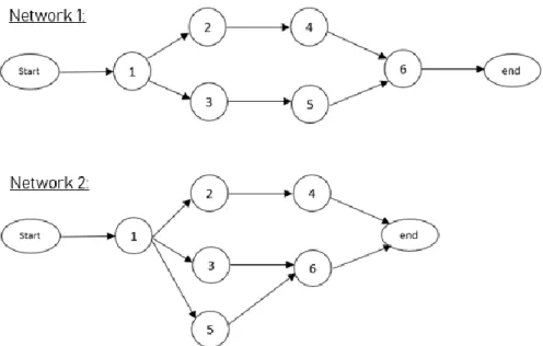
The variable “serial or parallel” (SP) indicates how the project network path is structured. This indicator takes a value closer to 1 when the network path takes a more serial or linear path, and a value closer to 0 when the network path knows a more parallel shape. In Figure 1, the first network will have smaller SP-coefficient than the indicator of the second network, i.e. the first network has a less parallel progress compared to the second network.

(12)

3

1.1.2 Project buffers

One of the most important objectives for the project manager and his team is to complete the project in time. This is highlighted by sometimes extremely high penalty costs. This implies that every project manager needs to consider both external and internal events that can influence its duration. Internal and external events may result in a longer duration than planned. External events represent for example delays in the supply of materials or unfavourable weather conditions. Internal events are for instance employee absenteeism or human errors. Buffer management focuses on how to take into account this uncertainty about future events. It helps the project manager to make the project more robust by adding buffers in the project schedule. The buffers are only consumed when events or factors affect the project schedule, other than the events or factors that could be foreseen or estimated during the planning phase. The impact and possible outcomes of buffer management is elaborated by Hu et al. (2015) and Hu et al. (2016), Vanhoucke (2012), and Martens (2018). When focussing on the time-aspect of our project, project buffers and feeding buffers can be added to increase the ability of the project to cope with unforeseen events. For an in-depth analysis of project buffer management, we encourage the reader to consult Buffer management methods for project control (Martens, 2018). For more information about how to determine the buffer size, we refer to Vanhoucke (2016) and section

2.3.1.

Network 1:

(13)

4

1.2 Scheduling Risk Analysis (SRA)

Due to risk and uncertainty, the actual duration of activities and thus the project completion will differentiate from this baseline scheduling. SRA analyses the sensitivity of the project activities and the project in general in terms of duration, due to uncertainty.

The analysis consists of four steps. First, the baseline scheduling needs to be constructed in order to serve as a reference value. In this step, a certain level of uncertainty is already covered by the PERT method, quantified in the different activity duration estimates. Second, statistical knowledge is required to understand the implications of risk and uncertainty, in order to take it into account when making conclusions. Third, Monte Carlo simulations generate durations for each activity that can be used to deviate from the original baseline scheduling with more empirically proved activity durations. This results in the fourth and last step, in which different sensitivity measures are analysed. The criticality index (CI) indicates the probability that the corresponding activity is situated on the critical path. Critical or not, different activities have an underlying relative importance, which is represented in the significance index (SI). The correlation of each activity’s duration on the project duration is captured in the cruciality index (CRI). Ballesteros-Pérez, Vanhoucke et al. (2019) made a performance comparison of these metrics. Although these indicators are very useful to understand the project one is dealing with, they are less important for this research topic. However, they can serve the project manager in two ways: they can indicate which activity is the most important when corrective actions need to be taken and they can be used to follow up the importance of activities when changes are made to the schedule during the project.

1.3 Project control

“Project control is the data gathering, management and analytical processes used to predict,

understand and constructively influence the time and cost outcomes of a project or program through the communication of information in formats that assist effective management and decision making”,

(PMI definition, Al Raee (2018)).

In other words, by applying project control, deviations of the planned schedule can be noticed during the project. These deviations occur in terms of budget performance and scheduling performance. The focus in this research is on the latter. We will introduce some tracking variables that allow the project manager to follow up his project. These variables are updated every time period, representing the current status of the project. The tracking variables need some tolerance limits, indicating what values are accessible in order to speak of a project in control. We will discuss this further in section 1.3.1.2.

(14)

5

1.3.1 EVM

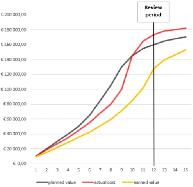
Earned value management (EVM) is the technique to monitor and evaluate the project progress at a higher level than individual activities. An overview of EVM-principles is given in Anbari (2003) and Fleming & Koppelman (2003) and Vanhoucke (2012). Its most important metrics are planned value, actual cost and earned value. These measures give us an indication of the (actual) performance of the project, which lead to the incentives for corrective actions. Because we compare time variables and costs variables, we want to obtain monetary values for all the measurements in order to compare these variables. Therefore, we need the budget-at-completion (BAC) which enables us to convert the time variables into monetary variables.

1.3.1.1 Key metrics

The planned value ratio (PV) is the forecasted cost for a certain time period t during the length of the project. The earned value (EV) can be compared to the planned value in order to determine if the project is still on track.

PV = Planned Percentage Of Completion ∗ BAC (1.3)

The actual cost measurement (AC) is very straight forward and means the cost that is already booked. This stands apart of any forecast. Tracking the actual expenses will enable us to compare the performance to the forecast, to determine if the project is on track.

Because AC only includes the costs made at a point in time, we need a ratio that deals with both money and completion. Because we are comparing financial numbers, we need a monetary value for this completion. This value is represented by the earned value (EV). This means that the EV at a certain time 𝑡 gives you the actual completion of the project (this completion-ratio is smaller than or equal to one) times the budget at completion.

(15)

6 In order to make a positive evaluation of the project at a certain time period t, the following constraints need to be respected:

AC ≤ EV (1.5)

PV ≤ EV (1.6)

In case of Figure 2, this means that both constraints are violated for 𝑡 =12, which means the project does not evolve as foreseen. Even the actual costs do exceed the planned costs.

Performance is measured and shown by variances. Two types of variances do occur: scheduling variance (SV) and cost variance (CV). Given that:

SV = EV – PV (1.7)

the scheduling variance is an indicator of delay in the project. If at a certain point in time PV > EV, which indicates that according to the schedule a larger amount of money was supposed to be spend, the positive value for SV points in the direction of a delay in the project. Vice versa, if SV equals a negative value, it means that the progression made so far is better than expected and that the project is ahead of schedule.

However, it might be that the analyst or project manager wants an answer to the question: “Does the project respect the given budget?”. Given that:

CV = EV – AC , (1.8)

the cost variance is an indicator of over- or underestimates of the costs of the different activities.

(16)

7 If AC > EV at a certain point in time, which indicates that the actual costs made until this moment are bigger than expected, it points in the direction of an underestimation of the costs of certain activities, and thus, the whole project.

Both SV and CV are important ratios, because they indicate the necessity of intervention. If so, corrective actions need to be taken to deal with delays or wrong estimates.

It is important to mention that the SV at the end of the project always equals 0. The planned percentage of completion and the real percentage of completion are supposed to be equal at the end of the project, which means SV equals 0, given equations 1.1, 1.2 and 1.5.

In this research topic, the emphasis lays on completion time. The earned schedule (ES) allows us to transform the monetary values such as PV, AC and EV into a time-based variable. In other words, ES tells you how the project is performing in terms of completion.

Each review period, the project is evaluated in terms of schedule performance. Answering the question “Is the project on track?”, various tracking variables can be used to test the null hypothesis. We refer to Martens (2018) for further analysis in depth. First, we need to analyse the difference between the actual progress and the planned progress. Therefore, we calculate the earned schedule (ES).

𝐸𝑆𝑡 = 𝑡 +

𝐸𝑉_𝑡 − 𝑃𝑉_𝑡

𝑃𝑉_𝑡+1− 𝑃𝑉_𝑡 (1.9)

Second, another tracking variable closely related to this ES, is the scheduling performance indicator:

𝑆𝑃𝐼 =𝐸𝑉 𝑃𝑉 (1.10) More specifically, 𝑆𝑃𝐼𝑡= 𝐸𝑆 𝐴𝑐𝑡𝑢𝑎𝑙 𝑡𝑖𝑚𝑒 (1.11)

will show at any time 𝑡 how close the project is to being completed compared to the planned schedule. Analog to the 𝑆𝑃𝐼, the cost performance indicator

𝐶𝑃𝐼 =𝐸𝑉

𝐴𝐶 (1.12)

indicates if the planned budget consumption is in line with the actual costs. For the latter formulas, a ratio that equals one indicates that respectively no delays(𝑆𝑃𝐼𝑡) or budget overruns are observed. Ratio’s smaller than one indicate that the project is behind schedule compared to what the project manager planned on beforehand. Ratios larger than one, however, indicate that the project is ahead on its planned progress. Both 𝑆𝑃𝐼𝑡 and 𝐶𝑃𝐼 can generate warning signals to indicate the project is out of control. However, in this research we do measure the impact of crashing on the completion time, and so there is less emphasis on the 𝐶𝑃𝐼. Although this measure is a very accurate performance

(17)

8 indicator, in order to determine if a project is on track, 𝑆𝑃𝐼𝑡 is meaningless when no boundary is set on its values. In other words, we need tolerance limits that indicate what range of values for the indicator result in accepting the null hypothesis.

1.3.1.2 Tolerance limits

Vanhoucke (2019) summarizes the types of tolerance limits. Martens & Vanhoucke (2017) and Colin & Vanhoucke (2014), next to giving an overview of the existing limits, came up with alternative approaches to construct tolerance limits, which set thresholds for different project tracking variables. Control charts are frequently used to show these tolerance limits graphically, at which critical points can be indicated. These approaches can be subcategorized into three main groups.

Static tolerance limits

The static control limits imply intuition. They are predetermined decision-making criteria, i.e. rules of thumb and they do not change over time. Goldratt (1997) suggested in his book ‘Theory of constraints’ the green-yellow-red system, a system where the consumption of the buffer in relation to the project completion is represented graphically. Three zones (yellow, green and red) are added to the graph to indicate the implications of the consumption for a certain observation. Predetermined conditions are applied to indicate if the corresponding buffer consumption is justified, depending on which zone the observation is plotted in. Leach (2005) suggests preparing corrective actions when the buffer exceeds the first third and to implement the actions when the buffer exceeds the second third.

Analytical tolerance limits

Analytical control limits are based on the different EVM metrics. Martens & Vanhoucke (2018) distinguish and evaluate four types of basic analytical limits: linear limits, cost limits, resource limits and risk limits. The most important differences compared to static control limits are that the control limits set thresholds and do change over time during different phases of the project, i.e. the control limit is adjusted to the actual status of the project. Next to these limits, the Relative buffer management approach (RBMA), introduced by Leach (2005), provides thresholds for the buffer consumption. It provides two tolerance limits. First, a limit that indicates if the buffer is able to support the entire project, the Relative Buffer Consumption Index (RBCI), defined by following formula:

𝑅𝐵𝐶𝐼 = 𝑃𝑟𝑜𝑝𝑜𝑟𝑡𝑖𝑜𝑛 𝑏𝑢𝑓𝑓𝑒𝑟 𝑐𝑜𝑛𝑠𝑢𝑚𝑒𝑑

𝑃𝑟𝑜𝑝𝑜𝑟𝑡𝑖𝑜𝑛 𝑜𝑓 𝑐𝑟𝑖𝑡𝑖𝑐𝑎𝑙 𝑐ℎ𝑎𝑖𝑛 𝑐𝑜𝑚𝑝𝑙𝑒𝑡𝑒𝑑 , (1.13)

which indicates if the buffer consumption at a certain moment in time is in proportion to the progress of the project at that time.

(18)

9 Second, a tolerance limit for the SPI and SV of a certain moment in time (t). These are control limits that are compared to the actual values of SPI and SV at that moment, and for which the actual values may not exceed these limits.

𝑆𝑃𝐼𝑡 = 100 100 + %𝑝𝑏 (1.14) 𝑆𝑉𝑡 = − %𝑝𝑏 100 + %𝑝𝑏∗ 𝑡 (1.15)

Martens & Vanhoucke (2017) proposes a new approach to determine the allowable buffer consumption at time 𝑡. This allowable consumption and the corresponding buffered planned progress (BPP), i.e. the planned value for the baseline schedule including a project buffer, are calculated as follows:

𝑎𝑏𝑡 = 𝑝𝑏 ∗ %𝑃𝑉𝑡 (1.16)

𝑤𝑖𝑡ℎ %𝑃𝑉𝑡=_𝐵𝐴𝐶𝑃𝑉𝑡

𝐵𝐵𝑃 = 𝑡 + 𝑎𝑏𝑡 (1.17)

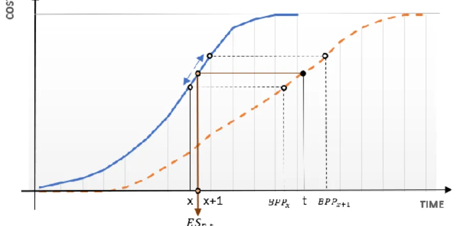
where 𝑎 is the allowable proportion of the buffer that may be consumed (i.e. proportional to the project completion) and where 𝑏𝑡 is the total available buffer. The corresponding tolerance limit for 𝑆𝑃𝐼𝑡does generate warning signals when the project seems to exceed its BPP and is constructed using the 𝐸𝑆𝑅,𝑡. In case the project manager inserted a buffer, the ES is adjusted in the following way:

𝐸𝑆𝑅,𝑡= 𝑥 +

𝑡 − 𝐵𝑃𝑃𝑥 𝐵𝑃𝑃𝑥+1 − 𝐵𝑃𝑃𝑥

(1.18)

where x corresponds to a time variable (situated on the PV-curve) that takes a value for which the condition 𝐵𝑃𝑃𝑥 ≤ 𝑡 and 𝐵𝑃𝑃𝑥+1 ≥ 𝑡 holds and 𝑡 corresponds to a time variable situated on BPP-curve.

Figure 3 provides a graphical representation of this equation. We do see that for a certain time 𝑡, we

can determine during which time interval [𝑥 ; 𝑥+ 1] the PV equals the BPP at time 𝑡.

(19)

10 The actual SPI(t) value will be compared to the required earned schedule (taking into account the project buffer), as discussed in section 1.4. No warning signal is sent when the following constraint holds: 𝑆𝑃𝐼𝑡 ≥ 𝐸𝑆𝑅,𝑡 𝑡 (1.19) 𝑤𝑖𝑡ℎ 𝐸𝑆𝑅,𝑡= 𝑥 + 𝑡 − 𝐵𝑃𝑃𝑥 𝐵𝑃𝑃𝑥+1 − 𝐵𝑃𝑃𝑥1 (1.20)

Statistical tolerance limits

Statistical process control (SPC) makes use of statistical principles to construct control limits and very often makes use of control charts. The main goal is to indicate if a process or project is in or out of control, by plotting observations of tracking variables and to subject them to control limits.

These limits can be based on either empirical (historical) data or on a desired state of progress. Both CPI and SPI are used to construct control charts with their corresponding control limits.

Colin and Vanhoucke (2014) give an overview of advanced statistical control limits that belong to the group making use of historical data. Control charts do represent the different outcomes of one variable during the project, subject to control limits which can be both static or dynamic, depending on the type of chart that is used. Lipke and Vaughn (2000) represent the tracked variable in an XmR-chart, in which the moving average is used to calculate the control limits to represent the random component of variation. As starting point to calculate these control limits, they make use of the CPI and SPI. With them, Bauch & Chung (2001), Leu & Lin (2008) and Aliverdi (2013) do make use of empirical data as input for their research. Colin and Vanhoucke do propose a new approach based on simulated data, that can be situated in the second group where the reference value for the observation is a desired state of progress. This approach provides (linear) tolerance limits that set thresholds for different EVM-metrics, i.e. allowable values in order to keep the process in control, which is fundamentally different from the control limits of SPC which indicate if a process is in control. Taking into account the status of the project and the desirable state of progress, the result are dynamic tolerance limits, that vary during the project.

(20)

11

1.4 Corrective actions

When warning signals do exceed their tolerance limits, or when external factors influence the product, the project manager may be urged to intervene to get the project back on track (if possible). Project Management Institute (PMI) defines corrective actions as follows: “any activity of action that is instituted, to bring the expected future performance of the project in line with the project management plan” (PMBOK, 2004). This definition emphasizes the intervening aspect of the corrective action and in that sense refers to altering specific tasks or series of tasks that are out of control, at different levels or in different domains. Kelly (2009) analysed triggers and possibilities to install corrective actions. Al Raee (2018) represents the implementation of corrective actions as an applied Deming wheel. Before the implemention and monitoring of the corrective action can take place, a root cause analysis identifies the appropriate actions with their advantages and disadvantages. Corrective actions can be reactive or proactive and are mostly approved by the management in the planning phase, however, they can be improvised at the moment itself. Proactive actions refer to actions that can avoid negative effects on activities, scheduled in the future when sensitivity metrics give warning signals. Reactive actions are actions that are triggered by performance indicator warning signals. On the project-level, a possible proactive corrective action is to negotiate the contract with the buying or selling institutions (for example extending the project deadline). On the activity-level we have many types of reactive corrective actions (Sharad, 1976). First, adjusting the network path by changing the sequence of performance of activities may have a positive impact on the project duration. This is referred to as fast tracking and implies to adjust the project network shape towards a more parallel shape. We refer to Vanhoucke & Debels (2008) for the in depth analysis. Meier et al. (2015) investigated how to implement activity crashing (see further on) and overlapping, Gerk & Qassim (2008) came up with a more complex algorithm for the crashing (see further on), substitution and overlapping of activities.

When it is not appropriate to alter the network shape, managers may control the baseline standard deviation, also referred as variability duration. Martens & Vanhoucke (2019) analysed its impact. Ensuring quality for example, foreseeing the appropriate equipment can positively impact the future scheduled activities to avoid negative effects, leading to increased activity durations and thus increased project durations.

In contrast to variability duration, the actual activity durations can be influenced. This last type of corrective actions is called activity crashing and implies reducing the activity duration. This reduction can be accomplished in many ways. Adjustments in the staffing can accelerate the project or keeping up the project with the original schedule, when it seems to deviate from this schedule. Next to this, providing more resources can be beneficial when needed in order to perform more activities at the

(21)

12 same time, or to accelerate one activity. Closely related to this, providing more money, i.e. enlarging the available budget, is mostly required to implement one of the previous actions. Every action comes with a cost, which implies that a certain budget can allow only a limited set of corrective actions, Martens & Vanhoucke (2019) call this the effort budget.

For of this research topic, the focus lies on activity crashing, i.e. the corrective actions result in the acceleration from certain activities and thus the project in general. Kelly (1961) and Fulkerson (1961) developed the period-by-period least marginal cost approach, where the algorithm tries to come up with the cheapest critical-path. Phillips & Dessouky (1977), Baker (1997), Jiang & Zhu (2010), Chen & Tsai (2011), etc. further elaborated this approach to improve the methodology. Johnson & Schou (1990), Bowman (2006) and Bregman(2009a) tried to adapt the decision-making of crashing for dynamic purposes. Analytically, the cost to crash time units is defined as follows:

𝑐𝑟𝑎𝑠ℎ 𝑐𝑜𝑠𝑡 𝑎𝑐𝑡𝑖𝑣𝑖𝑡𝑦𝑖 = (1.21)

𝑃 ∗ 𝑐𝑜𝑠𝑡 𝑝𝑒𝑟 𝑡𝑖𝑚𝑒 𝑢𝑛𝑖𝑡 ∗ (1 − 𝑐𝑟𝑎𝑠ℎ 𝑝𝑒𝑟𝑐𝑒𝑛𝑡𝑎𝑔𝑒) ∗ 𝑎𝑐𝑡𝑖𝑣𝑖𝑡𝑖𝑡𝑦 𝑑𝑢𝑟𝑎𝑡𝑖𝑜𝑛𝑖

Where P is the proportion of cost per time unit or in other words: the factor by which the standard cost per unit time is multiplied. In most cases, P will be equal or larger than one. The crash percentage equals the amount time units activityi that are crashed per corrective action.

Three methods are known to determine how to crash an activity. First, the brute force method: crashing the activity with the lowest activity cost, until the project is back on track or until a new critical path is found. Second, the linear programming method where the linear programming tool is able to come up with a solution where, including activity crashing, the completion time is minimised. Third, the traditional crashing method crashes the activity with the lowest crashing cost, situated on the critical path, until a stop criterion is fulfilled.

(22)

13

1.5 Monte Carlo simulation

In the past, several simulation models were developed to generate project outcomes, and to investigate the impact of crashing activities. Haga & Marold (2005) present a heuristic crashing algorithm using simulation, consisting of two steps. The first step is applying the PERT method to crash the project. In the second step, they test the impact of crashing the activities that can still be crashed. They focus on project control and suggest a method to determine at which moments the project should be evaluated in order to decide on crashing possibilities. Khul & Tolentino-Peña (2008) elaborates this further and comes up with a method to determine at which moments to crash and to do this in an optimal way, i.e. the optimal crashing strategy.

Van Slyke (1963) introduced Monte Carlo simulation principles to project management. Burt & Garman (1971) and Adlakha (1986) further elaborated this topic into a conditional Monte Carlo technique. The Monte Carlo simulation enables researchers to come up with a representative solution, by generating a wide range of possible outcomes. In essence, it means that a certain model is simulated an enormous number of times to fizzle out types of deviations. The necessary condition for this method is that the underlying distribution is known. As discussed in section 1.1, the activity durations follow a triangular distribution, characterised by the following probability density function:

The outcome when applying Monte Carlo simulations is based on the principle of Central Limit Theorem (CMT) (appendix A). For a sufficiently large sample size, the mean of all the samples will be close to or equal to the population mean. Next to that, the theorem states that when the sample size increases, every distribution of samples (in this case project outcomes) follows a normal distribution. This implies that in this case the simulation will result in an overall mean value with corresponding confidence interval for the completion time of the simulated project that can be used as input for the statistical analysis.

(23)

14

Chapter 2: Research methodology

2.1 Hypothesis testing

To quantify the research question in a statistical context and to be able to perform a statistical analysis using our results as input to come up with an answer, we define the null hypothesis (𝐻0) and the corresponding alternative hypothesis (𝐻1). These hypotheses reflect upon the delay that occurs without crashing and the delay when crashing is allowed.

𝐻0: The delay of projects without crashing does not significantly differ from

the delay of projects with crashing

𝐻1: The delay of projects without crashing does significantly differ from

the delay of projects with crashing

In order to measure the impact of activity crashing on the project outcome, the results of our simulation need to be tested towards a reference value. The reference value in this case is the project delay when the project is not altered during its execution. In other words, a comparison is set up between the project delay when the manager does not intervene the project, and the project delay when project interventions during review moments may appear. The delay is the positive difference between the actual project time and the project deadline (planned duration plus buffer) and equals zero if the project is on time. We cannot predict the exact value for the project completion and the corresponding project delay. However, we can estimate the range of values where the exact value can be situated, with (1-α)% certainty, where α is defined as the significance level, i.e. the probability that you will reject the null hypothesis although the null hypothesis is true (in statistical context, also referred to as Type I errors). Given that our completion time can be accelerated or can be delayed, the project outcome can be worsened or can be improved. This range of possible outcomes is represented in a two-sided confidence interval, in which the real delay may be situated, calculated according to the formula: 𝑐𝑜𝑛𝑓𝑖𝑑𝑒𝑛𝑐𝑒 𝑖𝑛𝑡𝑒𝑟𝑣𝑎𝑙 = [𝑋̅ − 𝑧𝛼 2 𝜎 √𝑛 ; 𝑋̅ + 𝑧𝛼₂ 𝜎 √𝑛] (2.1)

Where 𝑋̅ represents the mean delay (expressed in hours) in the sample after performing a Monte Carlo simulation.

𝑥 =

∑𝑛𝑖=1(𝑝𝑟𝑜𝑗𝑒𝑐𝑡 𝑑𝑒𝑙𝑎𝑦)𝑖

𝑛

(2.2)

𝑤ℎ𝑒𝑟𝑒 (𝑝𝑟𝑜𝑗𝑒𝑐𝑡 𝑑𝑒𝑙𝑎𝑦)𝑖> 0 𝑖𝑓 𝑝𝑟𝑜𝑗𝑒𝑐𝑡 𝑖𝑠 𝑙𝑎𝑡𝑒 = 0 𝑜𝑡ℎ𝑒𝑟𝑤𝑖𝑠𝑒

(24)

15 𝑛 = 𝑠𝑎𝑚𝑝𝑙𝑒 𝑠𝑖𝑧𝑒

𝜎 = 𝑠𝑡𝑎𝑛𝑑𝑎𝑟𝑑 𝑑𝑒𝑣𝑖𝑎𝑡𝑖𝑜𝑛 𝑜𝑓 𝑠𝑎𝑚𝑝𝑙𝑒

𝑧𝛼 = 𝑠𝑡𝑎𝑛𝑑𝑎𝑟𝑑 𝑑𝑒𝑣𝑖𝑎𝑡𝑖𝑜𝑛 𝑖𝑛 𝑛𝑜𝑟𝑚𝑎𝑙 𝑑𝑖𝑠𝑡𝑟𝑖𝑏𝑢𝑡𝑖𝑜𝑛 𝑔𝑖𝑣𝑒𝑛 𝑠𝑖𝑔𝑛𝑖𝑓𝑖𝑐𝑎𝑛𝑐𝑒 𝑙𝑒𝑣𝑒𝑙 𝛼 The significance level in our research is set on 0,05. Table A.1 in appendix A provides us with the corresponding value for the factor 𝑧𝛼/2, which equals 1,96 for the two-sided confidence interval. For further research about statistical hypothesis testing and how to use simulation in decision making processes we do refer to Gujarati & Porter (2009) and Law (2015).

2.2 Data set

The database for this project exists out of 900 projects provided by OR-AS. Each of these files contain 32 activities and four types of required resources. These resources do have a capacity of ten units. For each of the activity durations, predecessors and the number of required units of each resource are predetermined. This implies that also the network shape (SP) for each of these projects is known. To distinguish clearly whether we are dealing with a parallel or serial network shape, we distinguish three groups. The files for which the SP-indicator take a value lower than 0,3 define parallel networks. When the SP-indicator takes a value higher 0,7 we are dealing with serial networks. The networks of the files in between are considered as not significantly parallel or serial. This results in 300 projects per group. It is important to notice that in this simulation study, we do not take into account resource requirements, i.e. there are no resource constraints during the execution of projects. Activities can be executed from the moment that all of their predecessors are completed.

2.3 Design

Every project has its own characteristics. The possibilities are endless. However, we will limit our scope to only certain types of projects, by creating different cases using design factors. For each of these cases, the null hypothesis will be tested. We distinguish two types of design factors: static design factors which will determine what type of project is simulated (SP-value, budget, buffer size, lateness penalty cost) and dynamic factors that define the effort invested in corrective actions (number of review periods, number of corrective actions, crash costs). For these dynamic factors, different values are applied on the cases defined by the static factors to determine the impact of each factor. The range of values we do consider as input values are summarized in Table A.2 in appendix A. In the following sections, we will explain some of the assigned values.

2.3.1 Static design factors

With static design factors, each project is assigned its specific characteristics. These characteristics are static, i.e. they will not change over time during the project.

(25)

16 The first static design factor concerns the network shape (SP-value), explained in section 1.1. These networks are predetermined for our simulation study. The Critical Path Method determines the network path. Given these network shapes, the next design factor makes a distinction by assigning the available budget to each project. The project needs not only relevant, but also realistic input factors if we want to obtain research results which are meaningful for project management. In order to do so, we use earlier research to get realistic values for our input factors. Batselier and Vanhoucke (2015) have constructed a database that contains projects, applicable in project management studies. They created a database where the completion cost for most of the elements ranged between €100.000 and €5.000.000, for which the critical chain contained 85 activities on average. Given that our network paths only contain 32 nodes in total, we take €150.000 as reference value for the project budget. These budgets are used to determine activity costs. By dividing the budget by the sum of individual activity distributions, we get a cost per unit of time. In order to get the activity cost we multiply the cost per unit of time by the amount of time units the corresponding activity consumes.

𝑐𝑜𝑠𝑡 𝑝𝑒𝑟 𝑡𝑖𝑚𝑒 𝑢𝑛𝑖𝑡 = 𝑏𝑢𝑑𝑔𝑒𝑡

∑(𝑎𝑐𝑡𝑖𝑣𝑖𝑡𝑦 𝑑𝑢𝑟𝑎𝑡𝑖𝑜𝑛)𝑖 (2.3) 𝑎𝑐𝑡𝑖𝑣𝑖𝑡𝑦 𝑐𝑜𝑠𝑡𝑖=

𝑐𝑜𝑠𝑡

𝑢𝑛𝑖𝑡 𝑡𝑖𝑚𝑒∗ 𝑡𝑖𝑚𝑒 𝑢𝑛𝑖𝑡𝑠 𝑎𝑐𝑖𝑡𝑣𝑖𝑡𝑦𝑖 (2.4)

This design factor, however, will be less prominent as design factor in this research topic, because its impact will rather be small. Next to the planned budget, penalty costs for exceeding the deadline can be taken into account. This penalty can be fixed or can be variable. Fixed penalty costs are lump sums, activated whenever the project is late, where variable penalty costs implies an increasing cost per day the project is late. According to Hickson (2015) the penalty cost per time unit equals on average 2% of the total estimated project cost. The lateness penalty may be a decision-making factor for corrective actions, given that it reflects being one time-unit late. But because the focus in this research lies on time reduction by increasing crashing effort, lateness penalties are only referred to as an additional cost upon planned budget. From an economical point of view, when there are indications that a project is late, i.e. the planned duration at time t≠0 exceeds the planned duration estimated at an earlier time period, corrective actions will be taken if and only if the lateness penalty exceeds the increase in corresponding activity costs for this corrective actions. The increase in activity costs due to reduce activity durations equals the activity crashing cost. We recall formula 1.21 for the activity crashing cost in section 1.4:

𝑐𝑟𝑎𝑠ℎ 𝑐𝑜𝑠𝑡 𝑎𝑐𝑡𝑖𝑣𝑖𝑡𝑦𝑖= 𝑃 ∗ 𝑐𝑜𝑠𝑡 𝑝𝑒𝑟 𝑡𝑖𝑚𝑒 𝑢𝑛𝑖𝑡 ∗ 𝑎𝑐𝑡𝑖𝑣𝑖𝑡𝑖𝑡𝑦 𝑑𝑢𝑟𝑎𝑡𝑖𝑜𝑛𝑖∗ (1 − 𝑐𝑟𝑎𝑠ℎ 𝑝𝑒𝑟𝑐𝑒𝑛𝑡𝑎𝑔𝑒) This crash cost is normally compared to the penalty cost in order to decide if reducing the activity durations is reasonable from an economical point of view. However, because we want to measure the impact of activity crashing, we will crash either way whenever the 𝑆𝑃𝐼𝑡 generates warning signals,

(26)

17 even when the penalty cost advises otherwise. Depending on the value of the crashing percentage, we are able to construct different scenarios. These demonstrate the impact of the crash cost, which will form a restriction together with the budget on how much corrective actions can be taken. In this research, the crash percentage is arbitrarily set on crashing 30% of the remaining activity duration. The corresponding increase of cost per time unit (𝑃) is arbitrarily set on 200%.

The last static design factor is the size of the buffer. Although different types of buffers are explored in literature, we opt to insert an aggregated buffer at the end of the project. This will be consumed when activities of the critical path are having a delay. Three main approaches are considered to determine the size of the buffer. First, the rule-of-thumb 50% buffer, introduced by E. Goldratt, where the allowable project duration equals 150% of the planned project duration. More general and second, an arbitrary buffer may be inserted, where the allowable project duration is a multiplication of the planned project duration where the multiplying factor in our case varies between 0 and 0,5. Thirdly, a more analytical buffer can be inserted, based on triangular distributed activity durations. Vanhoucke (2016) provides more details about the so-called Root Squared Error Method (RSEM). The buffer is determined by the squared root of the sum of the quadratic deviations of the activity durations from the activities that are situated on the critical path.

𝑏𝑢𝑓𝑓𝑒𝑟 𝑠𝑖𝑧𝑒 = √∑(𝑝𝑒𝑠𝑠𝑖𝑚𝑖𝑠𝑡𝑖𝑐 𝑑𝑢𝑟𝑎𝑡𝑖𝑜𝑛 𝑎𝑐𝑡𝑖𝑣𝑖𝑡𝑦𝑖− 𝑜𝑝𝑡𝑖𝑚𝑖𝑠𝑡𝑖𝑐 𝑑𝑢𝑟𝑎𝑡𝑖𝑜𝑛 𝑎𝑐𝑡𝑖𝑣𝑖𝑡𝑦𝑖)2 (2.5)

2.3.2 Dynamic design factors

The first dynamic design factor is the number of review periods. A review period is a moment of evaluation during the project, where the project manager analyses and monitors the project progress and if necessary, adjusts the planned schedule. In this case, the project manager will determine if the project is in control by applying earned value management (section 1.3). When the metrics indicate a delay and thresholds generate warning signals, the project manager will consider corrective actions. This will possibly change the network path for a further iteration, which will be tested in a following review moment. The only question left is: how many times do you insert a review period? In order to evaluate the impact of different review patterns, we will cover four scenarios, shown in Figure 4. In the first scenario, review periods will occur at a constant interval. This means that at every interval 𝑡 (with 𝑡 >0), the progress will be evaluated. In the second scenario, the project manager wishes to follow up the project in its early stages, so the interval by which review periods occur, variates during the project. The interval is smaller in the early project stages and becomes larger towards the end of the project. In the third scenario in contrast, the project manager wants to follow up the project more towards the end than in the beginning. Here the interval will thus be larger in the early stages and

(27)

18 smaller towards the end. The last scenario is each time the default case, i.e. the case without review periods.

The second dynamic design factor is the number of corrective actions performed each review period. By performing more corrective actions, a different outcome in terms of project duration is possible. When a review period occurs, we will investigate the impact from performing one, two or three corrective actions. The last dynamic design factor is the activity crashing budget. We saw that a higher crashing cost influences the decision-making process of when to take corrective actions. By adjusting the crashing budget, we eliminate possible illimited crashing and thus an unrealistic crashing approach. However, the latter is used as default case, in other words a reference value to measure the impact of limiting the crash budget. We first limit the crash budget to an extra 5% of the planned budget. Next, we will decrease the crash budget even more to 2,5% of the planned budget. Given that the crash cost per time unit equals 200% of the activity cost without crashing and the budget equals €150.000, the crash percentages correspond with respectively 40- and 20- time units that can be crashed.

2.3.3 Review periods and corrective actions

In our design, the review periods will always take place. However, dependent on the tolerance limits, it might not be needed to intervene the project schedule. When the project arrives at a point in time where a review period is planned, the SPI(t) value will be compared to the required earned schedule (taking into account the project buffer), as discussed earlier in section 1.3.1.2.

We recall the tolerance limit (formulas 1.19 & 1.20). When the following constraint holds: 𝑆𝑃𝐼𝑡 ≥ 𝐸𝑆𝑅,𝑡 𝑡 𝑤𝑖𝑡ℎ 𝐸𝑆𝑅,𝑡 = 𝑥 + 𝑡 − 𝐵𝑃𝑃𝑥 𝐵𝑃𝑃𝑥+1 − 𝐵𝑃𝑃𝑥1

it is not necessary to intervene. However, if the 𝑆𝑃𝐼𝑡 value would result in a lower value, the project is off track and the predetermined number of corrective actions are taken, on the condition that the remaining budget allows the actions. We will apply the brute force crashing method discussed in

section 1.4 where we do crash the first activity we encounter on the critical path. However, we will not

(28)

19 always crash activities until the project is back on track. For each corrective action, we will reduce the activity duration of the first encountered critical activity by 30% of the remaining activity duration. When more than one corrective action is performed at one review period, one iteration consists of determining the critical path (which can change after crashing a certain activity) and performing the crashing of the duration.

The simulation framework distinguishes different types of projects at which the dynamic factors can be applied. The following five types of projects will be tested:

Type 1: Projects with more parallel networks (SP < 0.3) with an arbitrary buffer (10% or 20%) Type 2: Projects with more parallel networks (SP < 0.3) with an RSEM-based buffer

Type 3: Projects with nor parallel nor serial networks with an arbitrary buffer (10% or 20%) Type 4: Projects with nor parallel nor serial networks with an RSEM-based buffer

Type 5: Projects with more serial networks (SP > 0.7) with an arbitrary buffer (10% or 20%) Type 6: Projects with more serial networks (SP > 0.7) with an RSEM-based buffer

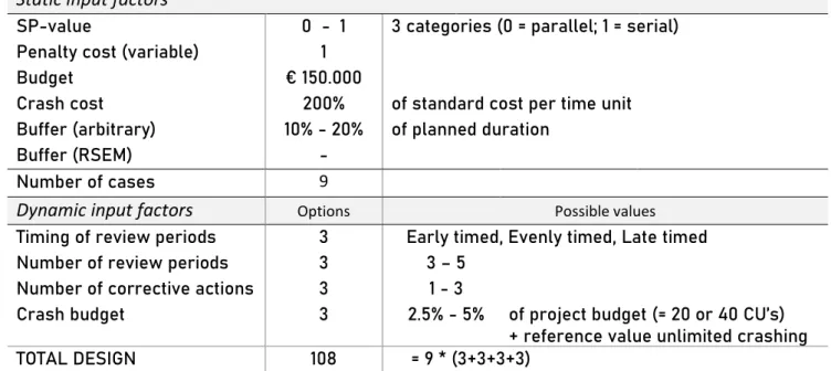
These types of projects result in 9 cases (three SP-categories in combination with three possible buffer sizes). Table 1 summarizes the dynamic factors that are applied to each of these cases, resulting in 108 cases of which the project outcome is simulated. In section 2.2, we assigned each SP-category 300 projects. Each case will be run 100 times, which results in 30.000 observations per case. This high amount of runs is necessary to obtain steady state values, i.e. values that are

representative for the corresponding project type. The activity duration distributions follow a triangular distribution (10,50,40) with 90% activity duration when the optimistic scenario holds and 140% activity duration in the pessimistic scenario.

Table 1: Design factors

Static input factors

SP-value 0 - 1 3 categories (0 = parallel; 1 = serial)

Penalty cost (variable) 1

Budget € 150.000

Crash cost 200% of standard cost per time unit

Buffer (arbitrary) 10% - 20% of planned duration

Buffer (RSEM) -

Number of cases 9

Dynamic input factors

Options Possible values

Timing of review periods 3 Early timed, Evenly timed, Late timed

Number of review periods 3 3 – 5

Number of corrective actions 3 1 - 3

Crash budget 3 2.5% - 5% of project budget (= 20 or 40 CU’s)

+ reference value unlimited crashing

(29)

20

2.4 Simulation

The data set (Patterson-files) provided by the Operations Research and Scheduling research group of Ghent University (OR-AS) serves via P2Engine input-functionalities as input for the simulation study, where a Monte Carlo simulation is performed in order to generate multiple outcomes for these given projects. These files are used to construct the baseline schedules and to monitor the project. P2Engine is a control tool developed by OR-AS, making use of the LUA scripting language. Vanhoucke (2014) gives an overview of its functionalities and opportunities, which are accessible via www.p2engine.com. The tool is able to construct the baseline schedule and tracking both risk analysis- and control or dynamic project metrics, by incorporating algorithms in ProTrack, the project management and software tool based on research by the OR-AS group. Because of its user-friendliness, it is frequently used in simulation studies. When constructing files using the LUA programming language, the programming terminal can call functionalities defined in the P2Engine tool and assign required input values to each variable. For every case that is investigated, the outcome of the corresponding projects is simulated 100 times. When input has been read, the simulation tool generates the project progress. Recall the probabilities {10, 50, 40} assigned to the triangular distribution, where the optimistic activity duration equals 90% of the standard duration and the pessimistic duration equals 140% of the standard duration. The project is evaluated and monitored at predetermined review periods, using the EVM-metrics. These review periods can be executed using the “callback”-function, provided by P2Engine, which is able to pause the simulation. The 𝑆𝑃𝐼𝑡-threshold (section 1.3.1.2) triggers corrective actions when exceeded. The crashing algorithm for one review period advances as follows:

a) Search for all activities that are busy or will start before the next review period b) Search for the activities that are situated on the current critical path

c) Crash the first encountered activity by X% of the remaining duration (in our case 30%)

d) If more than one corrective action may be taken, crash the next encountered activity until the allowed number of crashes per period is reached

Some restrictions need to be taken into account. Next to the predetermined crashing percentage, crashing is limited to the number of available crash units during that review period. For a given crash budget, the available crash units are equally spread amongst the review periods. If during one review period, the available crash units were not consumed, they are added to the available crash units in the next review period.

(30)

21

Chapter 3: Results and result analysis

In this chapter we try to provide the reader with insights when to invest effort in activity crashing. For different elements that determine the amount of crash effort, we investigate the impact on project outcomes. This chapter analyses the impact of investing effort in crashing time units in terms of delay reduction (expressed in hours) for projects that are late. We come up with rules of thumb for projects with different sizes of buffers and different network shapes, i.e. varying SP-categories, based on the activity distributions discussed in section 2.3. The results and simulation outcomes are either illustrated in this chapter by the use of graphs and tables, or in appendix B.

3.1 Hypothesis testing

The null hypothesis stated in the previous chapter is tested for each case. In appendix B.1 we provide the confidence intervals for both the delay of projects without crashing and the delay of projects when crashing is allowed if the threshold triggers corrective actions. Given the large amount of observations per simulation, these intervals are very accurate. This high accuracy results in the possibility to reject the null hypothesis each time, i.e. the confidence intervals per case do not overlap. Moreover, we may conclude that crashing activities significantly reduces the project delay. This allows us to look more in detail to its impact. The significance of crashing within each individual case allows us to compare the outcome of different settings in order to make proper conclusions. Because absolute deviations may result in biased conclusions during this comparison, we provide each time a performance measure that indicates the effectiveness of crashing by showing the ratio of delay reduction per crash unit.

3.2 Different buffer sizes

Each case is tested for three different buffer sizes (an arbitrary 10% buffer, an arbitrary 20% buffer and a buffer determined using the RSEM buffer) and three different SP-categories (see section 2.2). Before analysing the impact of each element individually, we may provide some general insights concerning arbitrary buffer sizes that hold for every element, when using the settings corresponding to the simulated projects. These insights can be verified for every element. First, when inserting an arbitrary buffer, we do see a clear difference in project outcome when inserting a buffer that increases the project deadline by 10% and when inserting a buffer that increases the project deadline by 20%. The predetermined activity distributions cause a certain delay in the project duration that can be carried by many projects with a 20% buffer. However, a 10% buffer in many cases is not enough to avoid exceeding the project deadline. This results for parallel projects (low SP-values) in three times more projects that are late when comparing 10% and 20% buffer for the same project. For higher SP-values, this difference can raise to even six times more projects late. Second, given the smaller delay for

(31)

22 projects with a 20% buffer, less delay needs to be eliminated by activity crashing. This results in less time units that are required to be crashed. In other words: investing more effort in crashing time units, i.e. increasing the number of crashed time units will be more effective to reduce the level of delays for projects with a 10% buffer compared to projects with a 20% buffer. This is why the performance measure results in systematically lower values for projects with the larger buffer. Third, next to the arbitrary buffer, we apply the same settings to projects which incorporate a buffer size based on the RSEM method. input. We notice that for higher SP-values five times more projects are late compared to projects with more parallel network shapes. When monitoring serial projects with the predetermined activity distributions, the RSEM method cannot foresee the project of a buffer that can absorb the delay.

3.3 Effort elements

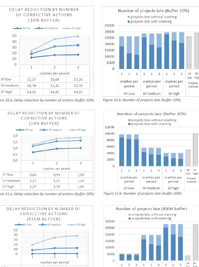
In the following sections, the reader is provided with graphical results for each effort-element. Three types of illustrations summarize the comparison between different settings per element. First, the level of delay reduction when crashing is shown on a graph. Next, the performance measure is summarized in a table. These two types add up to each other, as the performance measure does indicate if the extra effort really explains extra delay reduction. Lastly, the number of projects that are late with or without crashing are plotted in a bar chart and in addition, the number of projects that for which one or more corrective actions took place.

3.3.1 Impact of amount of crash budget

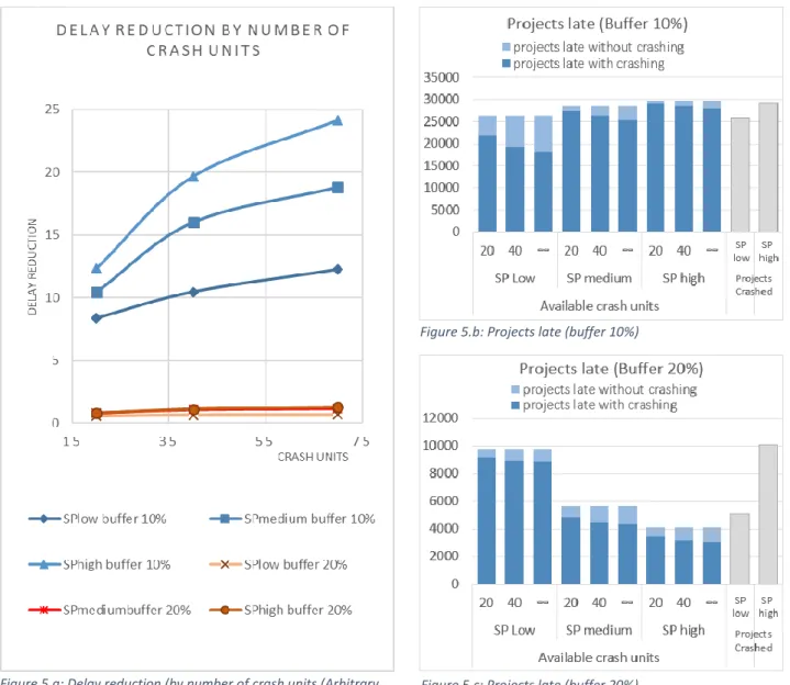
The bigger your crash budget, the more units of time that can be crashed, i.e. the bigger your effort is to get the project back on track. But this raises the question to which level crashing time units is effective. How big does your crash budget need to be? The goal of this section is to evaluate the impact of different sizes of the crash budget on project delay reduction. In section 2.3.2 is explained how the crash budget is converted into crash units (CU). The results of this section are summarized for 20 CU, 40 CU and a benchmark value where the total budget allows unlimited crashing.

First, we compare the outcomes for arbitrary buffers. In Figure 5.a, a higher crash effort results in higher delay reduction. However, the downward trend in the performance measure (Table 2) indicates that for these activity distributions less delay reduction per crash unit is obtained when foreseeing 40 CU’s compared to 20 CU’s. The declination is steeper for projects with lower SP-values. With a 10% buffer, the effectiveness ranges from 0.542 (for 20 CU) to 0.466 (for more CU’s). The decrease is less steep for projects with a 20% buffer: from 0.191 to 0.158 . Moreover, the performance measure

(32)

23 indicates that the level of effectiveness stabilizes when applying effort that equals 40 CU or more, given that the decline between 40 and unlimited CU’s is minimal. With a 10% buffer, the level of effectiveness for a certain level of crash budget is higher for increasing SP-values, while for projects with a 20% buffer the performance measure moves in opposite direction. The reason for this is twofold. First, when crashing time units in projects with parallel shapes, the critical path can change when other activities become critical when one of the original critical activities is crashed. For serial-shaped networks, crashing time units almost every time directly affects the original critical path and thus the project delay. Second, the predetermined activity distributions result with a 10% buffer in more delay that needs to be tackled for projects with higher SP-values and thus a bigger nominator in the ratio that provides the performance measure. The latter reason also explains why in Figure 5.b (when allowing crashing) a larger proportion of projects with a 10% buffer are finished on time for the lower SP-category compared to the higher SP-category. For projects with a 20% buffer the opposite is true (Figure 5.c).

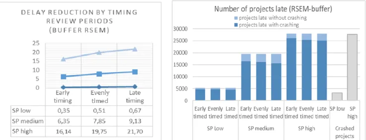
When the buffer size is determined using the RSEM buffer, we see a similar trend as with the arbitrary 10% buffer. The delay reduction increases when more effort is put in, but the effectiveness per crash unit decreases when investing more effort and stabilizes from 40 crash units on. As already mentioned in section 3.1, the level of effectiveness is higher when monitoring projects with more serial network shapes (i.e. higher SP-values). This higher level is explained by the delay that needs to be tackled. Recall that for serial projects with the predetermined activity distributions, the RSEM method cannot foresee the project of a buffer that can absorb the delay. The latter does also explain the clear difference in the number of projects that are crashed at one or more points in time between more serial (high SP) and more parallel (low SP) networks.

Buffer 10% Buffer 20% Buffer RSEM

20 CU 40 CU ∞ 20 CU 40 CU ∞ 20 CU 40 CU ∞

SP low 0,542 0,466 0,440 0,191 0,158 0,150 0,190 0,164 0,156

SP medium 0,631 0,603 0,597 0,159 0,141 0,134 0,428 0,400 0,392

SP high 0,701 0,685 0,692 0,148 0,135 0,130 0,635 0,615 0,617

(33)

24

Figure 5.a: Delay reduction (by number of crash units (Arbitrary buffer)

Figure 5.b: Projects late (buffer 10%)

Figure 5.c: Projects late (buffer 20%)

(34)

25

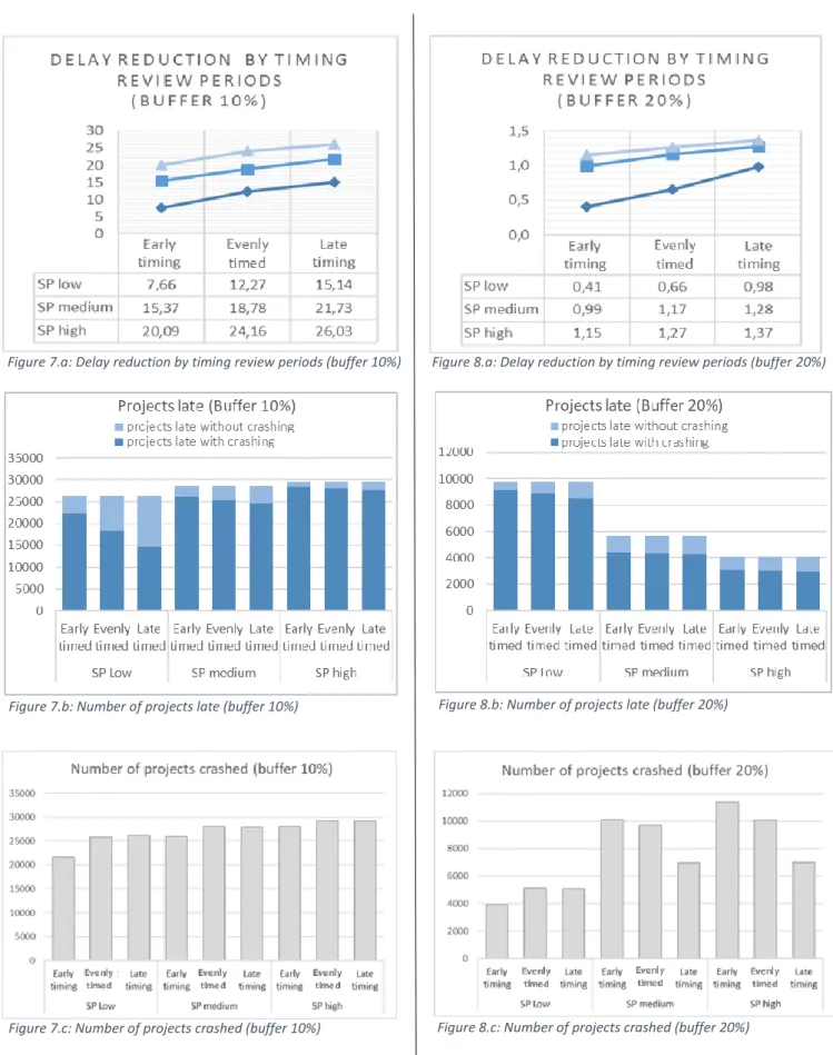
3.3.2 Impact of timing of review periods

In this section, we investigate if the timing of review periods may affect the effectiveness of crashing time units. When is it advised to evaluate the project and put effort in monitoring its progress? We will compare scheduling the review periods in the beginning, at the end or evenly spread during the project, as discussed in section 2.4, with one action per review period.

Both the arbitrary buffer sizes result in higher delay reduction when the review periods are placed towards the end of the project (Figures 7.a & 8.a). The performance measure in Table 3 adds to this.

Projects with a 10% buffer and serial network shapes result in performance values that range from 0.651 (when the project is monitored in the early stages), over 0.692 (when projects are monitored following a constant time interval) up to 0.720 (when the project is monitored towards the end). This analysis concludes that intervening the projects is most effective when it is reaching final stages. This is shown for projects with both arbitrary buffers and the buffer based on the RSEM method, in every SP-category. As shown in Figures 7.b, 8.b and 9.b, in one SP-category, more projects finish on time when projects are monitored more towards the end. When comparing one way of timing for different SP-categories, we see higher levels of effectiveness when crashing for increasing SP-values.

The number of projects where at least one activity is crashed one or more time units is shown in Figure

7.c. We see that with a 10% buffer for both serial and parallel networks rather the same number of

projects trigger activity crashing. However, when comparing the project completion times with and without crashing, a bigger proportion of extra projects finishes on time when dealing with lower SP-values compared to higher SP-SP-values. A whole other story holds when inserting a 20% buffer (Figure

8.c). The number of crashes performed in projects with lower SP-values is deviating from the other

categories and the proportion of extra projects that finish on time is bigger for projects with a more serial networks shape. The projects with a RSEM-based buffer are crashed more often if the project is more serial.

We may conclude that scheduling review periods more towards the end of the project increases the crash efficiency.

Buffer 10% Buffer 20% Buffer RSEM

Early timed Evenly timed Late timed Early timed Evenly timed Late timed Early timed Evenly timed Late timed SP low 0,340 0,440 0,459 0,119 0,150 0,206 0,127 0,156 0,197 SP medium 0,555 0,597 0,640 0,108 0,134 0,192 0,359 0,392 0,449 SP high 0,651 0,692 0,720 0,103 0,130 0,197 0,587 0,617 0,657

A simulation study on the effectiveness of investing effort in corrective actions to improve the project outcome