https://doi.org/10.5194/cp-14-1-2018
© Author(s) 2018. This work is distributed under the Creative Commons Attribution 4.0 License.
Signal detection in global mean temperatures after “Paris”:
an uncertainty and sensitivity analysis
Hans Visser1, Sönke Dangendorf2, Detlef P. van Vuuren1,3, Bram Bregman4, and Arthur C. Petersen5 1PBL Netherlands Environmental Assessment Agency, Bilthoven, the Netherlands
2Research Institute for Water and Environment, University Siegen, Siegen, Germany 3Faculty of Geosciences, University Utrecht, Utrecht, the Netherlands
4Institute for Science, Innovation and Society, Radboud University, Nijmegen, the Netherlands 5STEaPP, University College London, London, UK
Correspondence:Hans Visser (hans.visser@pbl.nl)
Received: 23 June 2017 – Discussion started: 6 July 2017
Revised: 5 December 2017 – Accepted: 8 December 2017 – Published:
Abstract.In December 2015, 195 countries agreed in Paris to “hold the increase in global mean surface temperature (GMST) well below 2.0◦C above pre-industrial levels and to pursue efforts to limit the temperature increase to 1.5◦C”. Since large financial flows will be needed to keep GMSTs be-low these targets, it is important to know how GMST has pro-gressed since pre-industrial times. However, the Paris Agree-ment is not conclusive as regards methods to calculate it. Should trend progression be deduced from GCM simulations or from instrumental records by (statistical) trend methods? Which simulations or GMST datasets should be chosen, and which trend models? What is “pre-industrial” and, finally, are the Paris targets formulated for total warming, originat-ing from both natural and anthropogenic forcoriginat-ing, or do they refer to anthropogenic warming only? To find answers to these questions we performed an uncertainty and sensitivity analysis where datasets and model choices have been var-ied. For all cases we evaluated trend progression along with uncertainty information. To do so, we analysed four trend ap-proaches and applied these to the five leading observational GMST products. We find GMST progression to be largely independent of various trend model approaches. However, GMST progression is significantly influenced by the choice of GMST datasets. Uncertainties due to natural variability are largest in size. As a parallel path, we calculated GMST progression from an ensemble of 42 GCM simulations. Mean progression derived from GCM-based GMSTs appears to lie in the range of trend–dataset combinations. A difference be-tween both approaches appears to be the width of uncertainty
bands: GCM simulations show a much wider spread. Finally, we discuss various choices for pre-industrial baselines and the role of warming definitions. Based on these findings we propose an estimate for signal progression in GMSTs since pre-industrial.
1 Introduction
Global mean surface temperature (GMST) is undoubtedly one of the key indicators of climate change. Tollefson (2015) denotes the GMST indicator as “the global thermostat”. Over the years many articles have been published in relation to GMST series and the patterns therein. These patterns com-bine an anthropogenic signal – induced by growing concen-tration of greenhouses and processes such as aerosol cool-ing – as well as natural variability. Natural variability can be regarded as a correlated noise process consisting of (i) in-ternal random unforced (chaotic) variability and (ii) exter-nal radiatively forced changes. Here, interexter-nal variability is steered by short-term processes such as weather in the high latitudes or El Niño and La Niña, as well as by decadal pro-cesses such as the Interdecadal Pacific Oscillation (e.g. Tren-berth, 2015; Fyfe et al., 2016; Xie, 2016; Meehl et al., 2016), and will result in correlated noise in GMSTs (Mudelsee, 2014; Roberts et al., 2015). Externally forced variability is mainly due to volcanic eruptions and variations in solar ir-radiance. It influences global temperatures on annual to cen-tennial scales (IPCC, 2013 – chap. 10; Forster et al., 2013;
2 H. Visser et al.: Signal detection in global mean temperatures after “Paris” Mann et al., 2016). A recent realization of internal
variabil-ity led to a fierce debate in the popular media: GMSTs were showing a claimed “slowdown”, “pause” or “hiatus” from the year 1998 onwards (e.g. Lewandowski et al., 2015; Hede-mann et al., 2017; Medhaug et al., 2017 – their Fig. 1).
GMST has been a crucial indicator in climate negotiations for a long time and it has even become more so at the fol-lowing 21st Conference of Parties (COP21) in Paris, De-cember 2015. The final accord, approved by 195 countries, agreed on GMST targets which aim to avoid increases of 1.5 and 2.0◦C compared to pre-industrial temperatures (UN, 2015). IPCC (2014) showed that meeting such GMST targets will require deep reductions of GHG emissions at the cost of high investments in mitigation measures worldwide. Given the fact that all goals are formulated on the basis of this sin-gle GMST indicator, the question arises: what is the current GMST level since pre-industrial?
So far, little attention has been paid to this topic. IPCC (2013), in its attempt to clarify the meaning of GMST measurements, applied linear trends to three differ-ent GMST datasets. They reported a trend progression 1µ of 0.85 [0.65, 1.06]◦C for the period 1880–2012. The uncer-tainty range stands for 90 % confidence limits, originating from differences in datasets, natural variability of the cli-mate system (forced and unforced). Hawkins et al. (2017) and Schurer et al. (2017) addressed the topic of trend pro-gression since pre-industrial and quantified the role of vari-ous choices for pre-industrial baselines.
Hawkins et al. found that the period 1720–1800 would be the most suitable in physical terms, despite incomplete information about radiative forcings and very few direct ob-servations during this time. Additionally, they concluded that the 1850–1900 period would be a reasonable surrogate for pre-industrial GMSTs, being only 0.05◦C warmer than the 1720–1800 period. Subsequently, Hawkins et al. analysed GMST progression since pre-industrial by calculating the GMST mean over the 20-year period 1986–2005 for various GMST products and other instrumental data (their Fig. 4). Trend progression itself was approximated in the study by multiple regression models with non-stationary explanatory variables such as historic GHG forcing curves or local tem-perature series (the Central England Temtem-perature series or the De Bilt series). Schurer et al. found that GHGs had a sig-nificant warming effect on global temperatures if the pe-riod 1401–1800 is compared to 1850–1900: from 0.02 to 0.20◦C (90 % confidence limits). If all forcings are combined (GHG, solar, volcanic), they found a similar warming effect of 0.09 [0.03–0.19]◦C.
In this article, we build on the work of Hawkins et al. but we do not base our GMST progression estimates on linear regression models with non-stationary regressors. The draw-back of this approach is simply the linearity assumed, while the climate system is (highly) non-linear with a number of feedback processes. The same holds for the approach pro-posed by Otto et al. (2015) and Haustein et al. (2017), who
apply temperature responses to (i) human-induced forcings and (ii) natural drivers as explanatory variables in a multiple regression model where the dependent variable is given by one of the observational GMST datasets.
Therefore, we follow two other trend estimation approaches: (i) statistical trend models and (ii) global temperature trends derived from global climate models (GCMs). Furthermore, we avoid methods or presentations based on subjectively selected time windows (such as Moving Averages). The drawback of time windows is that averages over 21-year periods or similar do not give estimates for the beginning and ending of the sample period chosen (thus, we would have no trend estimates for the period 2007–2016).
A final topic we address is that of warming definitions. Should the Paris targets be interpreted as warming due to both anthropogenic and natural forcings, or as warming due to anthropogenic warming only? The terms “global warm-ing” or “total warmwarm-ing” are interpreted in most literature as the sum of anthropogenic warming plus long-term (decadal to centennial) natural warming, consistent with the IPCC definition of climate change (IPCC Annex II, 2014). How-ever, some researchers interpret “global warming” as anthro-pogenic warming only, consistent with the definition pro-posed by UNFCCC in their article 1 (Otto et al., 2015; Haustein et al., 2017; Millar et al., 2017). In both definitions, short-term natural variability – such as seen in “the hiatus period” – is smoothed from warming trends.
Our approach is that of an uncertainty and sensitivity anal-ysis as promoted by Saltelli et al. (2004), Saisana et al. (2005) and Visser et al. (2015). We ask the following four major questions:
– How robust are estimates for GMST progression to cific choices of trend modelling, use of GCMs and spe-cific choices of GMST datasets?
– How do these choices influence uncertainties in GMST progression in relation to uncertainties due to forced and unforced natural variability?
– Does the choice for a specific pre-industrial baseline or period play a role?
– Does it matter if we interpret the Paris targets as total warming or as anthropogenic warming only?
Since there is no “true” or “best” trend approach (Visser et al., 2015), we explore four trend methods and apply these to five leading GMST products (similar to Hawkins et al.). This leads to a 4-by-5 matrix of GMST trend pro-gressions since 1880. As a parallel path, we compare these trend progressions to those deduced from GCMs. We anal-yse an ensemble of 42 GCM experiments from the Coupled Model Intercomparison Project phase 5 (CMIP5). GCMs are for a large part physics-based, in contrast to trend methods. However, there are also drawbacks, the main one being that
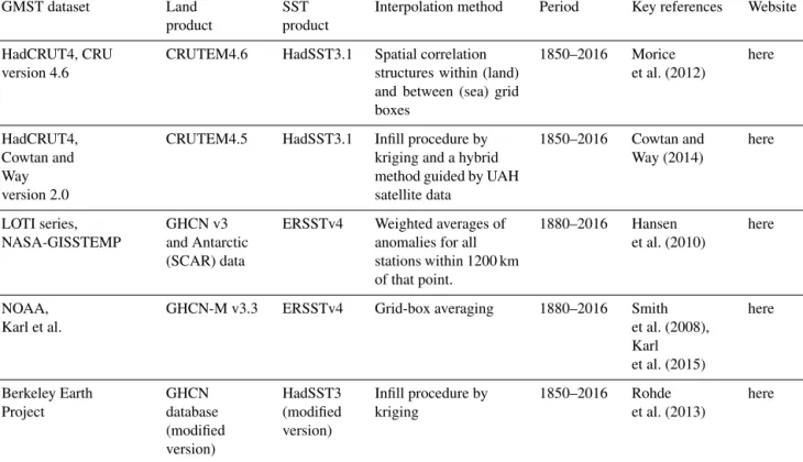
Table 1.Summary of observational datasets used in this study. Descriptions of interpolation schemes are only short indications. Details are given in the references.
GMST dataset Land
product
SST product
Interpolation method Period Key references Website
HadCRUT4, CRU version 4.6
CRUTEM4.6 HadSST3.1 Spatial correlation
structures within (land) and between (sea) grid boxes 1850–2016 Morice et al. (2012) here HadCRUT4, Cowtan and Way version 2.0
CRUTEM4.5 HadSST3.1 Infill procedure by
kriging and a hybrid method guided by UAH satellite data 1850–2016 Cowtan and Way (2014) here LOTI series, NASA-GISSTEMP GHCN v3 and Antarctic (SCAR) data
ERSSTv4 Weighted averages of
anomalies for all stations within 1200 km of that point. 1880–2016 Hansen et al. (2010) here NOAA, Karl et al.
GHCN-M v3.3 ERSSTv4 Grid-box averaging 1880–2016 Smith
et al. (2008), Karl et al. (2015) here Berkeley Earth Project GHCN database (modified version) HadSST3 (modified version) Infill procedure by kriging 1850–2016 Rohde et al. (2013) here
GCMs are only approximations to the real climate system and have considerable biases. Although GCMs are tuned to meet the main characteristics of the present climate (Voosen, 2016), GMSTs derived from GCMs still exhibit a wide range of trend progression estimates, as we will show.
In the discussion section, we address the role of various assumptions as for pre-industrial baselines, and differences in trend progression if Paris targets are interpreted as “total warming” vs. “anthropogenic warming”.
Our analysis is confined to historical data only (up to and including 2016). Examples for GMST projections have been given by IPCC (2013 – chap. 12), Forster et al. (2013), Mann (2014) and Schurer et al. (2017). A short-term prediction model is given by Suckling et al. (2016). An example of an uncertainty and sensitivity analysis of GMST projections has been given by Visser et al. (2000).
2 Data and methods
2.1 Data
Various research groups have published global GMST datasets. IPCC (2013 – Sect. 2.4.3) used three datasets, namely the HadCRUT4 series (Morice et al., 2012; Hope, 2016), the NOAA dataset (Vose et al., 2012) and the NASA/GISS dataset (Hansen et al., 2010). In the analysis here, we instead use a recent update of the NOAA data (Karl
et al., 2015). Karl et al. applied a number of corrections which mainly deal with sea surface temperatures, such as the change from buckets to engine intake thermometers. In addi-tion, we added two series, i.e. the version of the HadCRUT4 data in which the missing data have been filled in as pub-lished by Cowtan and Way (2014) and the GMST series by Rohde et al. (2013). Note that these datasets are not indepen-dent. They start from roughly the same station data over land, and more importantly are based on only two SST analyses: HadSST3 and ERSSTv4.
Cowtan and Way re-analysed the HadCRUT4 series by applying a statistical interpolation technique (kriging) and satellite data for regions where data are sparse. Their series shows higher GMST values in recent decades than the non-interpolated HadCRUT4 series due to the more-than-average warming of the poles. The land part of the GMST data of Rohde et al. (2013; Berkeley Earth group of researchers) systematically addressed major concerns of global warm-ing sceptics, mainly dealwarm-ing with potential bias from data selection, data adjustment, poor station quality and the ur-ban heat island effect. The ocean part (about 70 %) is taken from HadSST3. A summary of observational data products is given in Table 1.
Since two out of five GMST products start in the year 1880, we use the period 1880–2016 as our period of analy-sis. We return to this point in the discussion section. All data
4 H. Visser et al.: Signal detection in global mean temperatures after “Paris”
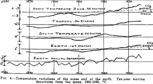
Figure 1.Graph taken from Callendar (1938). The fourth curve represents his GMST series, based on temperature data of 147 stations. To highlight smooth changes over time he used moving averages with a window of 10 years. It is interesting to note that he also addressed the specific effect of CO2emissions on global temperatures (dashed lines).
were downloaded from the institution websites with 2016 as the final year.
Next to these instrumental-data-based GMSTs we analyse three sets of GCM simulations all taken from CMIP5 (Tay-lor et al., 2012; IPCC, 2013 – chap. 9–12). GMST is defined here as the global average of near-surface temperature (tem-perature at surface, “tas”), in contrast to the observational datasets that use SST over sea for practical reasons (also de-noted as “blended temperature series”; Cowtan et al., 2015). The first set consists of GCM simulations where the input of greenhouse gases from 2005 onwards is taken from three representative concentration pathways (RCPs): 4.5, 6.0 and 8.5 W m−2(Van Vuuren et al., 2011; IPCC, 2014 – Sect. 12.4 and Fig. 12.5). These simulations cover the period 1861– 2100. We have taken a set of 42 GCM simulations with one member per model for emission scenario RCP4.5 (simula-tions for the other RCPs partly overlap with this set and are not considered here). GMSTs from CMIP5 simulations are based on wide range of modelling differences such as cli-mate sensitivities, cloud parametrization and aerosol forcing (e.g. IPCC 2013, chap. 9).
The second set that we have analysed, consists of 37 GCM runs for natural variability, denoted as “historicalNat”. These runs comprise forced and unforced natural variability but no GHG forcing (1860–2005). See Forster et al. (2013) for details. Finally, we analysed 41 pre-industrial control (Pi-Control) runs with lengths varying between 200 and 1000 years. These runs simulate natural internal variability only. All CMIP5 runs were downloaded from the KNMI Climate Explorer website with one member per model (Trouet and Van Oldenborgh, 2013).
2.2 Trend modelling
The tracking of signals or trends in GMST series has a long history. Callender (1938) studied in detail zonal and global temperatures, along with estimates for warming due to green-house gases (Fig. 1). To smooth changes he used moving av-erages with a window of 10 years. A wide range of methods have been applied since then to isolate long-term signals or “trends” in GMSTs. We have summarized trend techniques in Appendix A (Table A1).
As stated in the Introduction we choose statistical trend methods that allow for the quantification of trend progres-sion where no window is needed and where uncertainty esti-mates are available for any incremental trend value. Further-more, no specific period for pre-industrial has to be chosen (such as the mean of the 1851–1900 period or similar). “Pre-industrial” is reflected in the choice of the start of the sample period only.
Based on these considerations we have selected four trend approaches for our sensitivity analysis: ordinary least squares (OLS) linear trends, integrated random walk (IRW) trends and two approaches with splines. The first trend – a linear fit by OLS – was chosen by IPCC (2013) as their main method. Uncertainties simply follow from the linear model:
var(1µ2016) = var([a + b · 2016] − [a + b · 1880])
= var(137 · b) = 1372· var(b), (1)
where “a” is the intercept and “b” the slope. The variance of “b” follows from the OLS equations. Next to that the vari-ance estimate is corrected by calculating effective sample sizes Neff, based on annual data. This correction is important since residuals are not white noise due to persistence in natu-ral processes. The signal is therefore considered as noise with
1880 1900 1920 1940 1960 1980 2000 2020 Year -0.8 -0.4 0.0 0.4 0.8 Te m pe ra tur e anom al y (
C) HadCRUT4 GMT series Smoothing spline with DF = 7
1880 1900 1920 1940 1960 1980 2000 2020 Year -0.8 -0.4 0.0 0.4 0.8 (a) (b)
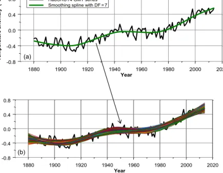
Figure 2.Construction of 1000 surrogate trend series by MC simulation, based on cubic splines. The AR(1) parameter estimated on the residuals of the spline model in (a) accounts for 0.28. A surrogate GMST series ˆyi,t is formed by simulating a new residual series ri,tbased
on the AR(1) process with ϕ = 0.28, and adding it to the estimated spline (green line in a). Then, a spline trend µi,t is estimated for each
surrogate ˆyi,t. As an illustration we have plotted 1000 of such trends µ1,t, . . ., µ1000,t in (b). Now, confidence limits can be estimated for
any µtbased on the values µ1,t, . . ., µ1000,t. These confidence limits can be based on SDs or percentiles. Similarly, confidence limits can
be calculated for the increment [µ2016−µ1880], based on the values [µ1,2016−µ1,1880], . . . , [µ1000,2016−µ1000,1880] (Mudelsee, 2014 –
Sects. 3.3.3 and 3.4).
a large decorrelation scale in this approach. The Neff correc-tion method has been explained by Zieba (2010), Chandler and Scott (2011, Sect. 3.3.3) and IPCC (2013 – 2SM).
The second trend approach that fulfils our uncertainty re-quirements, are sub-models from the class of structural time series models (STMs), in combination with the Kalman fil-ter (Harvey, 1989). From this group of models we choose the IRW trend model. The IRW trend model extends the lin-ear regression trend line by a flexible trend while retaining all uncertainty information (Visser, 2004; Visser et al., 2012, 2015). Furthermore, the flexibility of the trend model is opti-mized by maximum likelihood (ML) optimization. The IRW model reads as
yt=µt+εt and µt−2µt −1+µt −2=ηt, (2)
where yt denotes a measurement at time t and µt the trend component. The terms ηt and εt are independent, normally distributed white noise processes with zero mean.
The Kalman filter is the ideal filter here since it yields the so-called minimum mean squared estimator (MMSE) for the trend component in the model. The Kalman filter has been applied in many fields of research and is gaining popularity in climate research recently (e.g. Hay et al., 2015). As with OLS methods, residuals – or innovations in terms of the Kalman filter – should be white noise. We will use the Neffcorrection method in the case of correlated innovations (if necessary).
A third and fourth approach applies a combination of a trend model and the statistical structure of natural internal variability as derived from PiControl runs. It can be seen as a hybrid approach. To do so we have chosen the cubic spline trend model, a trend approach also applied in the AR5 (IPCC, 2013 – Box 2.2, Fig. 1). For a theoretical background we re-fer to Hastie et al. (2001) and Chandler and Scott (2011 – Sect. 4.1.3).
Smoothing splines are not statistical in nature and, thus, do not generate uncertainty estimates for GMST increments 1µ2016. However, uncertainty bands can be reconstructed by Monte Carlo (MC) simulations under the assumption of a given mean, variance and autocorrelation structure es-timated directly from the underlying dataset (Mudelsee, 2014 – Sect. 3.3). See Fig. 2 for an illustration.
To steer the flexibility of the cubic spline model we studied the correlation structure of internal variability. This correla-tion structure can be described by an AutoRegressive Mov-ing Average (ARMA) model as proposed by Hunt (2011) and Roberts et al. (2015). They estimated ARMA models to a range of PiControl runs. Similarly, we analysed 41 PiCon-trol runs with lengths varying between 200 and 1000 years. We found that variability can reasonably be characterized by AR(1) processes where the AR(1) parameter ϕ varies within the range [0.0, 0.75], depending on the GCM run chosen (see Mudelsee, 2014, Sect. 2.1). In this study we have removed
6 H. Visser et al.: Signal detection in global mean temperatures after “Paris” 1880 1900 1920 1940 1960 1980 2000 2020 Year -0.4 0.0 0.4 0.8 1.2 Trend increment 95% confidence limits [2016 - t ] ( C) 1880 1900 1920 1940 1960 1980 2000 2020 Year -0.04 -0.02 0.00 0.02 0.04 [t - t-1 ] ( C) Trend increment 95 % confidence limits 1880 1900 1920 1940 1960 1980 2000 2020 Year -0.6 -0.4 -0.2 0.0 0.2 0.4 0.6 0.8 Tempera tu re ano ma ly ( C) HadCRUT4 GMT series IRW trend 95 % confidence limits 1880 1900 1920 1940 1960 1980 2000 2020 Year -3.0 -2.0 -1.0 0.0 1.0 2.0 3.0 Inn ovati on s 0 5 10 15 20
Time lag in years -0.3 -0.2 -0.1 0.0 0.1 0.2 0.3 Corr el ati on (a) (c) (b) (d) (e)
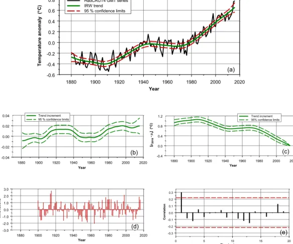
Figure 3.Results for the IRW trend model as applied to the HadCRUT4 series. Period: 1880–2016. Panel (a) shows the trend (green line) along with 95 % confidence limits (red dashed lines). The trend increments [µt−µt −1] are given in (b) along with uncertainties. Idem the
[µt−µ1880] values in (c). Panel (d) shows the innovations or one-step-ahead prediction errors which follow from the Kalman filter formulae.
Panel (e) shows the autocorrelation function (ACF).
the lowest and highest two ϕ estimates yielding the range [0.28, 0.60].
We note that in some cases MA(1) or ARMA(1,1) models performed somewhat better as checked by comparing AIC values. Thus, the AR(1) model is a compromise to ease the analysis. Next to that AR(1) models are widely applied in climate research (e.g. Mudelsee, 2014).
All four trend methods are designed to smooth GMSTs for annual to decadal natural variability (forced and un-forced). However, if Paris targets should be interpreted as anthropogenic warming only, we should estimate the role of decadal to centennial forcings from volcanic and solar ac-tivity as well. To estimate the role of volcanic eruptions we have extended the OLS linear trend model and the IRW trend model by adding the aerosol optical depth (AOD) index as regressor (Visser and Molenaar, 1995; Visser et al., 2015 – Fig. 4). The extended IRW model reads as
yt=µt+αxt+εt and µt−2µt −1+µt −2=ηt, (3a) where the variable xt stands for the inclusion of an explana-tory variable (regressor). The AOD index is available from
NASA for the period 1850–2016 (Sato et al., 1993; Ridley et al., 2014).
We note that if the variance of noise process ηt in model (3a) is set to zero, the model reduces to the OLS mul-tiple regression model with one regressor:
yt=α0+α1t + α2xt+εt. (3b)
Thus, model (3b) is a special case of model (3a).
3 Results
3.1 Sensitivity analysis trend methods and data products
Based on the 1880–2016 GMST sample period we have evaluated trend progression values 1µ2016from 1880 up to 2016 along with uncertainties for all datasets and trend ap-proaches. This yields the 4-by-5 matrix shown in Table 2. As for linear trends we corrected uncertainty estimates by a fac-tor√(1.60/0.40) = 2.0, analogous to the approach chosen
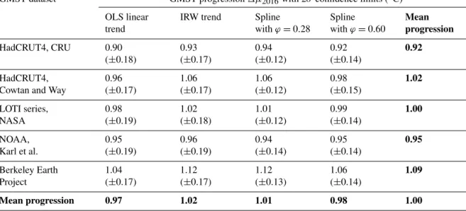
Table 2.Trend increments 1µ2016along with 2σ confidence limits. Increments are given for the five GMST series given in Table 1, and the
four trend approaches proposed in Sect. 2.2. Values in bold are row and column averages.
GMST dataset GMST progression 1µ2016with 2σ confidence limits (◦C)
OLS linear trend
IRW trend Spline
with ϕ = 0.28 Spline with ϕ = 0.60 Mean progression HadCRUT4, CRU 0.90 (±0.18) 0.93 (±0.17) 0.94 (±0.12) 0.92 (±0.14) 0.92 HadCRUT4, Cowtan and Way
0.96 (±0.17) 1.06 (±0.17) 1.06 (±0.12) 0.98 (±0.15) 1.02 LOTI series, NASA 0.98 (±0.19) 1.02 (±0.18) 1.01 (±0.12) 0.99 (±0.14) 1.00 NOAA, Karl et al. 0.95 (±0.19) 0.96 (±0.19) 0.94 (±0.14) 0.95 (±0.14) 0.95 Berkeley Earth Project 1.04 (±0.17) 1.12 (±0.17) 1.12 (±0.13) 1.06 (±0.14) 1.09 Mean progression 0.97 1.02 1.01 0.98 1.00
in IPCC (2013 – chap. 2, Supplement) since first-order au-tocorrelations lie around 0.60. Table 2 shows that the trend slopes for the datasets HadCRUT4, LOTI-NASA, NOAA-Karl and Cowtan and Way are close, where the lowest slope value is for the HadCRUT4 series. This dataset has poor cov-erage in the Arctic, where trends are much higher than the global mean. The steepest trend is found for the Berkeley Earth series. Identical patterns are found for the other trend models: lowest trend progression for the HadCRUT4 dataset and highest values for the Berkeley Earth dataset.
As for the IRW trend estimates – formulated in Eq. (2) – we find reasonable flexible patterns which closely resemble the spline trend shown in IPCC (2013 – chap. 2: Box 2.2, Fig. 1b). An example for the HadCRUT4 dataset is shown in Fig. 3. Data, trend and uncertainties are shown in the upper panel. The trend increments [µt−µt −1] and [µt−µ1880] are given in the middle left and right panel, respectively, along with uncertainties (see explanations given in Visser, 2004). The [µ2016−µ1880] value with uncertainty is taken as the value in Table 2. The lower left panel shows the innovations or one-step-ahead prediction errors which follow from the Kalman filter formulae. The lower right panel shows the au-tocorrelation function (ACF). We note that a prerequisite of Kalman filtering is that the innovations – also denoted as one-step-ahead prediction errors – follow a white noise process. The ACF shows an AR(1) value of 0.30 which is slightly significant. We applied the Neffcorrection for compensating for this the violation by applying the approach of IPCC, as we did for linear trends: uncertainty bands are corrected by a factor√(1.30/0.70) = 1.3.
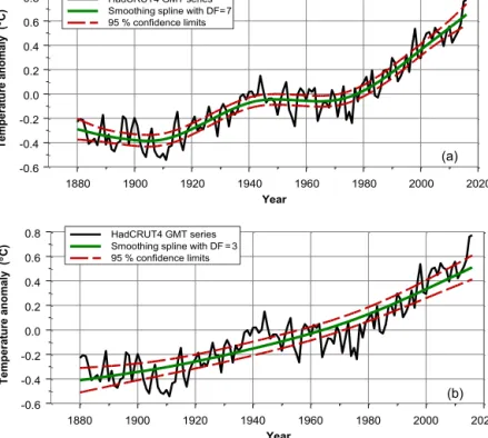
As for smoothing splines, we have estimated trends in GMST series such that the residual series exhibits an AR(1) process with a ϕ value of 0.28 and 0.60. Trend estimates
based on the HadCRUT4 series are shown in Fig. 3. The spline approaches show quite different trend patterns. The model shown in the upper panel of Fig. 4 is based on a slightly correlated noise process and – as for the IRW trend from Fig. 3 – closely resembles the spline trend shown in IPCC (2013 – chap. 2: Box 2.2, Fig. 1b). The model shown in the lower panel shows a parabolic shape. This parabolic pattern closely resembles the anthropogenic signal in GMST series as shown by IPCC (2013 – Fig. 10.1f), derived from “historicalGHG” simulation runs (Forster et al., 2013).
It is interesting to note that none of the four trend methods show a sign of a “hiatus”, “slowdown” or “pause”. That is not surprising for the linear trend and the spline estimate with ϕ =0.60 due to their stiff character. However, the IRW trend and spline with ϕ = 0.28 are more flexible and do not show any stabilization pattern for recent years at all. We tested the residuals of the IRW trend model and these appear to be close to white noise (see lower panels of Fig. 2). This inference is consistent with recent findings on the hiatus (Marotzke and Forster, 2015; Hedemann et al., 2017; Medhaug et al., 2017; Rahmstorf et al., 2017).
Table 2 shows that differences between trend model and dataset combinations can be considerable. The lowest 1µ2016 value is found for the HadCRUT4 dataset in com-bination with the IRW trend model: 0.90 ± 0.18◦C (± 2σ ). The highest values are found for the Berkeley Earth dataset in combination with cubic spline interpolation and ϕ = 0.28: 1.12 ± 0.13◦C. These two extremes reveal that the range of 1µ2016values due to datasets and trend models accounts for 0.22◦C. This range is somewhat lower than that due to nat-ural variability alone. Based on 2σ limits, we find a low es-timate of ± 0.12◦C, leading to a maximum range of 0.24◦C (LOTI dataset in combination with cubic spline interpolation
8 H. Visser et al.: Signal detection in global mean temperatures after “Paris” 1880 1900 1920 1940 1960 1980 2000 2020 Year -0.6 -0.4 -0.2 0.0 0.2 0.4 0.6 0.8 Tempera tu re ano ma ly ( C) HadCRUT4 GMT series Smoothing spline with DF = 3 95 % confidence limits 1880 1900 1920 1940 1960 1980 2000 2020 Year -0.6 -0.4 -0.2 0.0 0.2 0.4 0.6 0.8 Tempera tu re ano ma ly ( C) HadCRUT4 GMT series Smoothing spline with DF=7 95 % confidence limits
(a)
(b)
Figure 4.Two smoothing spline estimates for the HadCRUT4 GMST series, with uncertainties generated by MC simulation. All confidence limits are based on 1000 surrogate GMST series following the approach set out in Mudelsee (2014 – Sect. 3.3.3). (a) AR(1) parameter chosen as ϕ = 0.28 (equivalent to 7 degrees of freedom), the low end of ϕ values within CMIP5 PiControl runs. (b) AR(1) parameter chosen as ϕ =0.60, the high end of ϕ values (DF = 3).
and ϕ = 0.28), and a high estimate of ± 0.19◦C, leading to a maximum range of 0.38◦C (three combinations in Table 2). To quantify the role of trend methods in more detail we have averaged trend estimates over the five GMST datasets and added it to Table 2 (bottom row). It shows that the range of trend progressions is small: [0.97, 1.01]◦C. At the other hand, if we average over trend methods, the variability due to datasets is found (right column of Table 1). The variabil-ity accounts for [0.92, 1.09]◦C. Clearly, variability due to GMST datasets is dominant over specific trend approaches.
3.2 Trend progression derived from GCM simulations Trend progression derived from GCMs have been anal-ysed in a range of studies, e.g. IPCC (2013 – chap. 10), Forster et al. (2013), Marotzke and Forster (2015), Mann et al. (2016) and Meehl et al. (2016). Here, we derive trend progression since pre-industrial by taking an ensemble of 42 GCM all-forcing simulations 1861–2016. We note that underlying models have quite different characteristics, such as climate sensitivities, various models for greenhouse gas cycling models, cloud parametrization and aerosol forcing. However, we did not perform a sensitivity analysis for these factors.
Short-term forced and unforced natural variability in individual GCM simulations is smoothed by estimating
splines to each individual simulation (both for ϕ = 0.28 and ϕ =0.60, as in Fig. 4). In this way we find 42 values for 1i,2016≡yi,2016−yi,1861. Results are shown in Fig. 5 (based on smoothing splines with ϕ = 0.28). The mean 12016value is 1.17 ± 0.50◦C (2σ ) for smoothing all 42 curves with ϕ =0.28 and 1.01 ± 0.52◦C for smoothing with ϕ = 0.60. These values are consistent with those reported by Forster et al. (2013, Table 3).
The GCM simulations analysed here differ from data prod-ucts as for their definition of temperatures (“tas only” vs. blended temperatures). Cowtan et al. (2015) and Richard-son et al. (2016 – Fig. 1) showed that tas temperatures differ from blended temperatures by 0.10◦C, for the period 1860– 2009. Thus, mean GCM-derived warming estimates cover the ranges [1.00–1.15]◦C (tas) or [0.90–1.05]◦C (blended). We note that these ranges reasonably correspond to the range found in Table 2.
4 Discussion
4.1 Uncertainty and sensitivity analysis
We make three comments concerning the robustness of the results given in Sect. 3. First, as summarized in Table A.1 of Appendix A, a wide range of trend models exist in the lit-erature, all with varying characteristics. The fact that many
0.4 0.6 0.8 1.0 1.2 1.4 1.6 1.8 2.0 2016 relative to 1861 (C) 0 1 2 3 4 5 N um ber o f GC M m em ber s
Figure 5.Histogram based on 42 GCM 1i,2016values, relative to 1861. Mean value is 1.17 ± 0.50◦C (2σ ). Individual GCM curves were
smoothed by splines, where the AR(1) parameter is chosen as ϕ = 0.28 (equivalent to 7 degrees of freedom), the low end of ϕ values within CMIP5 PiControl runs.
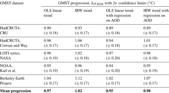
Table 3.GMST progression 1880–2016 with and without correction for volcanic activity (see Fig. 6). Values in bold are column averages.
GMST dataset GMST progression 1µ2016with 2σ confidence limits (◦C)
OLS linear trend
IRW trend OLS linear trend
with regression on AOD
IRW trend with regression on AOD HadCRUT4, CRU 0.90 (± 0.18) 0.93 (± 0.17) 0.89 (± 0.18) 0.89 (± 0.17) HadCRUT4,
Cowtan and Way
0.96 (± 0.17) 1.06 (± 0.17) 0.94 (± 0.18) 1.01 (± 0.17) LOTI series, NASA 0.98 (± 0.19) 1.02 (± 0.18) 0.97 (± 0.20) 0.98 (± 0.18) NOAA, Karl et al. 0.95 (± 0.19) 0.96 (± 0.19) 0.94 (± 0.20) 0.95 (± 0.19) Berkeley Earth Project 1.04 (± 0.17) 1.12 (± 0.17) 1.02 (± 0.17) 1.07 (± 0.17) Mean progression 0.97 1.02 0.95 0.98
of these methods are not statistical in nature does not limit their application in the present context: the approach shown in Fig. 2 (creating surrogate GMST series by MC simula-tion) is also applicable to methods such as binomial filters or LOESS estimators. Therefore, we cannot rule out that the influence of trend modelling is underestimated in Table 2. However, given the (i) small differences shown in the bottom row of Table 2, and (ii) the wide uncertainty bands due to natural variability, we judge such an underestimation to be relatively small.
A second comment concerns a source of uncertainty deal-ing with the choice for year or period that can be regarded as “pre-industrial”. As for the analyses in Sect. 3.1, we have chosen the year 1880 as low end of the sample period, simply because two out of five GMST products start in 1880 (NASA and NOAA). Both NOAA and NASA reason that SST data for the pre-1880 period are too sparse (Hansen et al., 2010 – indentation [15]).
The choice for 1880 is consistent with that made by IPCC (2013) as for historic trend progression (without claiming this to be “since pre-industrial”). In Sect. 3.2 we have chosen the year 1861 as low end of the sample period, again since simulations are available from that year onwards.
Would our results and conclusions from Table 2 or Figs. 3 and 4 be different if the sample period were enlarged, starting in 1400, 1720 or 1850? Strictly speaking, we cannot answer this question since we cannot extend our analyses to these starting years due to data availability. As for the instrumen-tal dataset, we could perform some analyses from 1850 on-wards but GMST estimates become inaccurate for these early decades. However, estimates based on GCM simulations are given by Hawkins et al. (2017) and Schurer et al. (2017).
Hawkins et al. show that the GMST difference between the two periods 1720–1800 and 1850–1900 is small, around 0.05◦C, lying on the edge of statistical significance. Ad-ditionally to their analysis we compared GMST mean
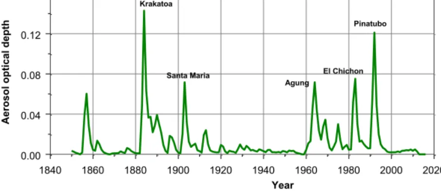
val-10 H. Visser et al.: Signal detection in global mean temperatures after “Paris” 1840 1860 1880 1900 1920 1940 1960 1980 2000 2020 Year 0.00 0.04 0.08 0.12 0.16 Ae rosol op tic al dep th Krakatoa Pinatubo Santa Maria Agung El Chichon
Figure 6.The AOD index series as introduced by Sato et al. (1993). Period is 1850–2016.
ues over three periods: 1850–1900, 1860–1880 and 1880– 1900, based on the HadCRUT4 dataset. The mean val-ues appear to be similar: −31 ± 0.03◦C, −0.31 ± 0.06◦C and −0.32 ± 0.05◦C, respectively (2σ limits). These dif-ferences are small if compared to the uncertainties due to natural variability, shown in Table 2. These results suggest that the choice for 1720–1800, 1850–1900, 1860–1880 or 1880–1900 as “pre-industrial” will have a small influence to the findings presented here. At the other hand, Schurer et al. show from GCM simulations that global warming is underestimated by 0.09 [0.03, 0.19]◦C if the period 1401– 1800 is chosen as pre-industrial baseline (compared to the period 1850–1900). Their estimate for the influence of GHG only lies close to these estimates, in the range from 0.02 to 0.20◦C. We conclude that recent simulations point to an underestimation of global warming if calculated relative to late nineteenth century estimates. The underestimation lies around 0.10◦C.
A third comment deals with differences in warming defini-tions as mentioned in the Introduction. If the Paris targets are to be interpreted as anthropogenic warming only, we should estimate these contributions as well. Clearly, the incremen-tal estimates 1µ2016 shown in Table 2 do not contain cor-rections for decadal to centennial natural forcings from solar and volcanic activity. To estimate the role of volcanic activity on the estimates given in Table 2 we have extended the OLS linear trend and the IRW trend model with a regression com-ponent, where GMST series are regressed on the OAD in-dex shown in Fig. 6, following models (3a) and (3b). Results are summarized in Table 3. The table shows that incremen-tal estimates 1µ2016are overestimated by 0.02◦C for linear trends and by 0.04◦C for IRW trends. A reason for this over-estimation could be the high volcanic activity for the period 1880–1890, containing the peak eruption of the Krakatoa).
To estimate the role of long-term solar activity we did not choose for the time-series approach above since any ex-planatory variable in a regression model with some long-term trend will correlate and “explain” the long-term trend in the dependent variable (the cyclic pattern in solar radiance is not
reflected in GMTs as shown by a number of studies, e.g. Schurer et al., 2017 – Fig. S3). Therefore, we prefer to use GCM estimates to quantify the role of solar activity.
IPCC (2013) estimates the role of solar variability to be small and on the edge of significance. Incremental solar forc-ing for the period 1750–2011 accounts for 2 [0, 4] % of GHG forcing (Figure SPM.5 and Box 10.2). Schurer et al. (2017 – Fig. S3) estimate the incremental contribution of solar forc-ing on GMSTs to be 0.07 [0.02, 0.12]◦C. This estimate com-pares the period 1850–1900 to 1990–2000. Furthermore, the long-term influence of volcanic activity is non-significant in their simulations (their Fig. S2).
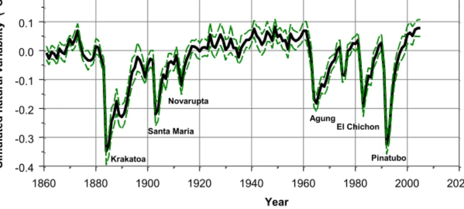
Next to these estimates we analysed an ensemble of 37 GCM simulations with natural forcing only (“historicalNat”; IPCC, 2013 – Figs. 10.1 and 10.7; Forster et al., 2013 – Fig. 2). The mean curve with 2 standard errors (SEs) is shown in Fig. 7, along with major volcanic eruptions (eruptions with a volcanic explosivity index of 5 and 6). Mean trend progres-sion for these 37 runs accounts for 0.078 ± 0.030◦C (2 SE), 1861–2005.
From these inferences we conclude that the difference be-tween total warming and anthropogenic warming lies around 0.10◦C with an uncertainty range of [0.0, 0.14].
4.2 Policy recommendation
Schurer et al. (2017) end their article with the recommenda-tion that a consensus be reached as to what is meant by pindustrial temperatures. In this way, the chance would be re-duced of conclusions that appear contradictory being reached by different studies. Furthermore, it would allow for a more clearly defined framework for policymakers and stakehold-ers. We fully agree with this recommendation. However, our uncertainty and sensitivity analysis has shown that the choice of a proper pre-industrial baseline is not the only parame-ter that could lead to contradictory results. Decisions around data products and GCM simulations, various time series techniques, or assumptions on warming definitions should be taken into account as well.
1860 1880 1900 1920 1940 1960 1980 2000 2020 Year -0.4 -0.3 -0.2 -0.1 0.0 0.1 0.2 S imula ted natu ra l va ri abi lity ( C) Agung El Chichon Santa Maria Krakatoa Novarupta Pinatubo
Figure 7.Natural variability based on 37 GCM simulations. Shown are mean values along with 2 standard errors. Period is 1861–2005.
Here, we make the following policy proposal which aims to be a reasonable compromise. First, we propose to base GMST warming estimates on data products rather than GCM simulations. Our argumentation is that 12016values based on GCM simulations show a wide range of warming estimates (Fig. 5). We note that even wider ranges are found for abso-luteGMST estimates (CMIP5 estimates for the mean GMST value over the period 1961–1990 show a range of 2.5◦C ac-cording to IPCC 2013 – Fig. 9-8). Another argument is that forcing estimates from CMIP5 are accurate up to the year 2005 (estimates for 2006–2016 apply to approximations for GHG concentrations, with no volcanic or solar activity).
Second, since warming estimates vary as a function of the GMST data products chosen (Table 2), we propose to esti-mate trends on the annual averages of all five data products.
Third, we found that the choice for specific trend methods plays a minor role, with largest differences between stiff and more flexible trend models. Therefore, we propose to apply a flexible and a stiff trend method and average the warming estimates found.
Fourth, two studies on the role of pre-industrial base-lines have been published recently. Schurer et al. (2017) find a GHG-induced warming in the range [0.02, 0.20]◦C if the period 1401–1800 is compared to the period 1850– 1900. Hawkins et al. (2017) define the period 1720–1800 as a reasonable baseline for pre-industrial and find small non-significant differences between the period 1720–1800 and 1850–1900. We choose to follow the baseline proposed by Hawkins et al. Since GMST observational data are uncertain in the pre-1880 period (sparse SST data) and GMST mean values for 1850–1900 and 1880–1900 appear to be of equal size (based on the HadCRUT4 data product), we propose to analyse trend progression from 1880 onwards.
Finally, we propose to interpret global warming in the context of “Paris” as the sum of natural and anthropogenic warming, consistent with the IPCC definition of climate change. One argument for this choice is that ecological sys-tems and human society will respond to total warming and induced shifts in climate extremes regardless of its origin.
From these choices it follows that trend progression 12016 accounts for 1.00 ± 0.13◦C (bottom row of Table 2). It is interesting to compare this estimate with that published re-cently by Haustein et al. (2017). They find for GMST warm-ing the incremental value 1.01 [0.87, 1.22]◦C, which is close to our findings. This is remarkable since their estimate is based on another approach and quite different assumptions.
5 Conclusions
We have addressed the issue of signal progression of GMST in relation to the GMST targets agreed upon in Paris in De-cember 2015. Although these targets are clearly defined – avoiding increments of 1.5 and 2.0◦C – there remain a num-ber of (scientific) questions unanswered in the agreement. We have identified five aspects of the accord which hamper an exact quantification of GMST progression: (i) the use of instrumental data and trend methods vs. GCM-derived pro-gression, (ii) the role of varying datasets, (iii) the role of varying trend methods, (iv) the role of varying choices for pre-industrial and (v) the role of warming definitions. Since there is no “true” or “best” approach (Visser et al., 2015), we have chosen to perform an uncertainty and sensitivity on GMST progression as propagated by Saltelli et al. (2004) and related articles. This allows us to test the robustness of vari-ous trend progression claims.
Approaches based on instrumental data.We find that trend values for GMST progression 1880–2016 vary considerably, from 0.90◦C (HadCRUT4 dataset in combination with the IRW trend model) to 1.12◦C (Berkeley Earth dataset in combination with cubic spline interpolation and ϕ = 0.28). The two extremes reveal that the range of 1µ2016 values due to datasets and trend models accounts for 0.22◦C. This range is smaller than that due to natural variability alone. Based on 2σ limits, we find a low estimate of 0.24◦C (LOTI dataset in combination with cubic spline interpolation and ϕ =0.28) and a high estimate of 0.38◦C (three combinations in Table 2). Furthermore, variability due to various GMST
12 H. Visser et al.: Signal detection in global mean temperatures after “Paris” products dominates the variability due to specific trend
ap-proaches.
Approaches based on GCMs. We find that mean trend progressions lie within the range of estimates from instru-mental data. However, the uncertainty bands for 42 simula-tions are much wider than those derived from instrumental trend estimates. Here, GCM variability stems from a wide range of modelling assumptions such as climate sensitivities, cloud parameterization and aerosol forcing (e.g. IPCC, 2013, chap. 9), in addition to natural variability.
The choice of a pre-industrial period. Recent studies have shown that GHG warming prior to 1880 or 1850 can-not be neglected. Schurer et al. (2017) estimate that early warming (1401–1800 compared to 1850–1900) accounts for 0.09 [0.03, 0.19]◦C. The role of solar and volcanic activity is minimal in this comparison.
Interpretation of Paris targets as being “total warming” or “anthropogenic warming only”. We find that the role of solar and volcanic activity is small on centennial scale. This contribution lies around 0.10◦C (0.03◦C from volcanic ac-tivity and 0.07◦C from solar activity; see Sect. 4.1 for an explanation).
Hiatus. As a side result of our trend analyses we note that no signs of an “hiatus”, “slowdown” or “pause” can be discerned in GMST trend progression. This inference is consistent with recent findings (Marotzke and Forster, 2015, Hedemann et al., 2017, Medhaug et al., 2017, Rahmstorf et al., 2017).
Policy recommendation. Schurer et al. (2017) recom-mend that a consensus be reached as to what is meant by pre-industrial temperatures. Our analysis shows that other sources of uncertainties should be taken into account as well. If not, contradictory results will appear in different studies with direct consequences for CO2reductions to hold GMSTs below the Paris targets. Our proposal shows a GMST pro-gression 12016of 1.00◦C.
Code availability. IRW trends have been estimated by the TrendSpotter software. This software package is freely available from the first author. Splines have been estimated by the statistical package S-Plus, version 8.2. The scripts, which are highly similar to R, are available from the first author.
Data availability. All five GMST datasets are open access and have been downloaded from the authors websites. All CMIP5 runs named in Sect. 2.1 were downloaded from the KNMI Climate Ex-plorer website with one member per model (Trouet and Van Old-enborgh, 2013). The names of individual GCMs can be found there as well. Please see https://climexp.knmi.nl/cmip5_indices.cgi?id= someone@somewhere. Data used for the graphical presentations in this article can be gained from the first author.
Appendix A: An overview of trend methods, applied to GMST observational data
In our study we have selected trend models which not only estimate a trend over time but also yield uncertainties for trend increments. However, this requirement appears to limit our model choices considerably. First, many methods are not statistical in nature, such as moving averages (Hansen et al., 2010; Smith et al., 2015; Fyfe et al., 2016), binomial filters (Morice et al., 2012), wavelets with scale dependencies (Lin and Franzke, 2015), EEMD decomposition (Wei et al., 2015; Yao et al., 2015) or linear trends based on stair-step averages with variable lengths (De Saedeleer, 2016). A historic exam-ple is given in Fig. 1, based on the work of Callender (1938). Next to that, a number of methods do not generate es-timates at the beginning and ending of the GMST series due to the dependence on “windows”. Examples are moving averages, OLS linear trends with moving windows (Risbey et al., 2015; Marotzke and Forster, 2015) and the staircase approach by De Saedeleer (2016).
Trend models applied to GMST datasets can be catego-rized methodological into three groups:
– Empirical models. These are trend models which are in principle data-based and may be steered by qualitative physical insights, such as the choice of a fixed window in combination with moving averages (Easterling and Wehner 2009; Hansen et al., 2010; Cowtan and Way, 2014; Roberts et al., 2015). Other trend models are OLS linear trends with varying sample periods (IPCC, 2013 – Box 2.2, Fig. 1a; Karl et al., 2015; Rajaratnam et al., 2015), linear trends with change points (Cahill et al., 2015), binomial filters (Morice et al., 2012), splines (IPCC, 2013 – Box 2.2, Fig. b), EEMD decomposition (Wei et al., 2015; Yao et al., 2015), structural time series models (Visser and Molenaar, 1995; Mills, 2006, 2010) and long-memory trend models (Lennartz and Bunde, 2009; Rea et al., 2011).
– Semi-empirical methods with stationary regressors. These methods are also data-based but physics may en-ter trend estimates by adding stationary climate indices in the context of regression models. An example is given by Forster and Rahmstorf (2011), who apply a linear re-gression model with three regressors (MEI, AOD and TSI). Other references are Visser and Molenaar (1995), Yao et al. (2015) and Trenberth (2015).
– Semi-empirical methods with non-stationary regressors. These models differ from semi-empirical models in that non-stationary regressors are used as well, such as global CO2 emissions. Typical examples are given by Imbers et al. (2013) and Hawkins et al. (2017). An ex-ample where GMST data are treated as regressor to model global sea levels has been given by Rahmstorf (2007).
A detailed description of methods is given in Table A1. For background information please see Chandler and Scott (2011), Mudelsee (2014) and Visser et al. (2015).
From the range of available trend methods we selected trend methods from the group of empirical models and semi-empirical models, with our main selection criterion being that models contain full uncertainty information for trend es-timates and trend increments. Based on this criterion we se-lected Models (4), (8), (16), (19) and (21). As for Model (8) we explained the construction of uncertainties in Fig. 2.
Furthermore, we decided not to use models from the semi-empirical approaches with non-stationary regressors. First, there is a danger of finding associations rather than causal re-lations since any two series with a long-term trend correlate high, whatever their origin (Nuzzo, 2014). Second, relations in the climate system are (highly) non-linear and we prefer to rely on GCM simulations rather than forcing indicators for GHGs, aerosols or solar activity which serve as regressors in a multiple regression model. Thus, we prefer the mod-els named in Table A1 under the heading “Semi-empirical approaches, stationary regressors” over “Semi-empirical ap-proaches, non-stationary regressors”.
14 H. Visser et al.: Signal detection in global mean temperatures after “Paris”
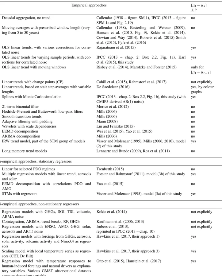
Table A1.Summary of three groups of modelling approaches to global mean temperatures: (i) empirical, (ii) semi-empirical with stationary regressors, and (iii) semi-empirical with non-stationary regressors. In the fourth column the presence of uncertainties for rates of change is given ([µt−µs] ± ?). The term “not explicitly” means that uncertainties could be calculated in principle but not shown by the author(s).
Empirical approaches [µt−µs]
±?
1 Decadal aggregation, no trend Callendar (1938 – figure SM.1), IPCC (2013 – figure
SPM.1a and Fig. 2.19)
no
2 Moving averages with prescribed window length
(vary-ing from 5 to 50 years)
Callendar (1938), Easterling and Wehner (2009), Hansen et al. (2010, Fig. 9), Kokic et al. (2014), Cowtan and Way (2014), Roberts et al. (2015) Smith et al. (2015), Fyfe et al. (2016)
no
3 OLS linear trends, with various corrections for
corre-lated noise
Rajaratnam et al. (2015) yes
4 OLS linear trends for varying sample periods, with
cor-rections for correlated noise
IPCC (2013 – chap. 2: Box 2.2, Fig. 1a), Karl et al. (2015), this study
yes
5 OLS linear trend with moving windows Risbey et al. (2014), Marotzke and Forster (2015) only for
[µt−µt −1]
6 Linear trends with change points (CP) Cahill et al. (2015), Rahmstorf et al. (2017) not explicitly
7 Linear trends, based on stair step averages with variable
lengths
De Saedeleer (2016) yes, by colour
graphs
8 Splines with Monte Carlo simulation IPCC (2013 – chap. 2: Box 2.2, Fig. 1b), this study (with
CMIP5-derived AR(1) noise)
yes
9 21-term binomial filter Morice et al. (2012) no
10 Hodrick–Prescott and Butterworth low-pass filters Mills (2006) no
11 Smooth transition trends Mills (2006) no
12 Adaptive filtering with padding Mann (2008) no
13 Wavelets with scale dependencies Lin and Franzke (2015) no
14 EEMD decomposition Wei et al. (2015), Yao et al. (2015) no
15 ARIMA decomposition Mills (2006) no
16 IRW trend model, part of the STM group of models Visser and Molenaar (1995), Mills (2006, 2010), model
(2) of this study
yes
17 Long memory trend models Lennartz and Bunde (2009), Rea et al. (2011) no
Semi-empirical approaches, stationary regressors
18 Linear for selected PDO regimes Trenberth (2015) no
19 Multiple regression models with linear trend, aerosols
and solar
Forster and Rahmstorf (2011), model (3b) of this study yes
20 EEMD decomposition with correlations PDO and
AMO
Yao et al. (2015) no
21 STMs with regressors Visser and Molenaar (1995), model (3a) of this study yes
Semi-empirical approaches, non-stationary regressors
22 Regression models with GHGs, SOI, TSI, volcanic,
ARMA noise
Kokic et al. (2014) not explicitly
23 Cointegration, ARIMA, trend breaks, RF, GHGs Kaufmann et al. (2006, 2013) not explicitly
24 Regression models with ENSO, AMO, GHG, solar,
aerosols and AR(1) noise
Imbers et al. (2013),
reprinted in IPCC (2013 – chap. 10)
not explicitly
25 Regression models with forcings from GHGs, aerosols,
solar activity, volcanic activity and Nino3.4 as regres-sors
Hawkins et al. (2017, their approach 1) yes
26 Scaling model with local temperature series as
regres-sors (CET, De Bilt)
Hawkins et al. (2017, their approach 3) yes
27 Regression model with temperature responses to
human-induced forcings and natural drivers as explana-tory variables. Various GMST observational datasets serve as dependent variable.
Competing interests. The authors declare that they have no con-flict of interest.
Acknowledgements. We thank Geert Jan van Oldenborgh (KNMI, Climate Explorer) for thorough comments on an early version of this text. Furthermore, we thank Peter Thorne (Maynooth University), an anonymous reviewer and Lenny Smith (The Lon-don School of Economics and Political Science) for important comments on the manuscript.
Edited by: Stefan Bronnimann
Reviewed by: Peter Thorne and one anonymous referee
References
Cahill, N., Rahmstorf, S., and Parnell, A. C.: Change points of global temperature, Environ. Res. Lett., 10, 084002, https://doi.org/10.1088/1748-9326/10/8/084002, 2015.
Callendar, G. S.: The artificial production of carbon dioxide and its influence on temperature, Q. J. Roy. Meteor. Soc., 64, 223–240, 1938.
Chandler, R. E. and Scott, E. M.: Statistical Methods for Trend De-tection and Analysis, Wiley & Sons Statistics in Practice, West Sussex, UK, 2011.
Cowtan, K. and Way, R. G.: Coverage bias in the HadCRUT4 tem-perature series and its impact on recent temtem-perature trends, Q. J. Roy. Meteor. Soc., 140, 1935–1944, 2014.
Cowtan, K., Hausfather, Z., Hawkins, E., Jacobs, P., Mann, M. E.,
Miller, S. K., Steinman, B. A., Stolpe, M. B., and
Way, R. G.: Robust comparison of climate models with observations using blended land air and ocean sea sur-face temperatures, Geophys. Res. Lett., 42, 6527–6534, https://doi.org/10.1002/2015GL064888, 2015.
De Saedeleer, B.: Climatic irregular staircases: generalized accel-eration of global warming, Nature Scientific Reports, 6, 19881, https://doi.org/10.1038/srep19881, 2016.
Easterling, D. R. and Wehner, M. F.: Is the climate
warm-ing or cooling?, Geophys. Res. Lett., 36, L08706,
https://doi.org/10.1029/2009GL037810, 2009.
Forster, G. and Rahmstorf, S.: Global temperature
evo-lution 1979–2010, Environ. Res. Lett., 6, 044022,
https://doi.org/10.1088/1748-9326/6/4/044022, 2011.
Forster, P. M., Andrews, T., Good, P., Gregory, P. M., Jackson, L. S., and Zelinka, M.: Evaluating adjusted forcing and model spread for historical and future scenarios in the CMIP5 generation of cli-mate models, J. Geophys. Res.-Atmos., 118, 1139–1150, 2013. Fyfe, J. C., Meehl, G. A., England, M. H., Mann, M. E., Santer, B.
D., Flato, G. M., Hawkins, E., Gillet, N. P., Xie, S. P., Kosaka, Y., and Swart, N. C.: Making sense of the early-2000s warming slowdown, Nat. Clim. Change, 6, 224–228, 2016.
Hansen, J., Ruedy, R., Sato, M., and Lo, K.: Global
sur-face temperature change, Rev. Geophys., 48, RG4004,
https://doi.org/10.1029/2010RG000345, 2010.
Harvey, A. C.: Forecasting, Structural Time Series Models and the Kalman Filter, Cambridge University Press, Cambridge, UK, 1989.
Hastie, T., Tibshirani, R., and Friedman, J.: The Elements of Sta-tistical Learning, Springer series in statistics, New York, USA, 2001.
Haustein, K., Allen, M. R., Forster, P. M., Otto, F. E. L., Mitchell, D. M., Matthews, H. D., and Frame, D. J.: A real-time global warming index, Nature Scientific Reports, 7, 15417, https://doi.org/10.1038/s41598-017-14828-5, 2017.
Hawkins, E., Ortega, P., Suckling, E., Schurer, A., Hegerl, G., Jones, P., Joshi, M., Osborn, T., Masson-Delmotte, V., Mignon, J., Thorne, P., and Van Oldenborgh, G.:
Es-timating changes in global temperature since the
pre-industrial period, B. Am. Meteorol. Soc., 98, 1841–1856, https://doi.org/10.1175/BAMS-D-16-0007.1, 2017.
Hay, C. C., Marrow, E., Kopp, R. E., and Mitrivica, J. X.: Prob-abilistic reanalysis of twentieth-century sea-level rise, Nature, 517, 481–484, 2015.
Hedemann, C., Mauritsen, T., Jungclaus, J., and Marotzke, J.: The subtle origins of surface-warming hiatuses, Nat. Clim. Change, 7, 336–339, 2017.
Hope, M.: Temperature spiral goes viral, Nat. Clim. Change, 6, 657–657, 2016.
Hunt, B. G.: The role of natural climatic variation in perturbing the observed global mean temperature trend, Clim. Dynam., 36, 509–521, 2011.
Imbers, J., Lopez, A., Huntingford, C., and Allen, M. R.: Testing the robustness of the anthropogenic climate change detection statements using different empirical models, J. Geophys. Res.-Atmos., 118, 3192–3199, 2013.
IPCC: Climate Change 2013: The Physical Science Basis. Con-tribution of Working Group I to the Fifths Assessment Report of the Intergovernmental Panel on Climate Change, edited by: Stocker, T. F., Qin, D., Plattner, G. K. Tignor, M. M. B., Allen, S. K., Boschung, J., Navels, A., Xia, Y., Bex, V., and Midgley, P. M., Cambridge University Press, Cambridge, 2013.
IPCC: Climate Change 2014: Mitigation of Climate Change. Con-tribution of Working Group III to the Fifths Assessment Report of the Intergovernmental Panel on Climate Change, edited by: Edenhofer, O., Pichs-Madruga, R., Sokona, Y., Minx, J. C., Fara-hani, E., Kadner, S., Seyboth, K., Adler, A., Baum, I., Brunner, S., Eickemeier, P., Kriemann, B., Savolainen, J., Schlöner, S., Von Stechow, C., and Zwickel, T., Cambridge University Press, Cambridge, 2014.
IPCC Annex II: Glossary, Contribution of Working Groups I, II and III to the Fifth Assessment Report of the IPCC, edited by: Pechauri, R. K. and Meyer, L. A., IPCC, Geneva, Switzerland, 2014.
Karl, T. R., Arguez, A., Huang, B., Lawrimore, J. H., McMahon, J. R., Menne, M. J., Peterson, T. C., Vose, R. S., and Zhang, H.: Possible artifacts of data biases in the recent global surface warming hiatus, Science, 348, 1469–1472, 2015.
Kaufmann, R. K., Kauppi, H., and Stock, J. H.: Emissions, con-centrations, and temperature: a time series analysis, Climatic Change, 77, 249–278, 2006.
Kaufmann, R. K., Kauppi, H., Mann, M. L., and Stock, J. H.: Does temperature contain a stochastic trend: linking statistical results to physical mechanisms, Climatic Change, 118, 729–743, 2013. Kokic, P., Crimp, S., and Howden, M.: A probabilistic analysis of human influence on recent record global mean temperature changes, Clim. Risk Management, 3, 1–12, 2014.
16 H. Visser et al.: Signal detection in global mean temperatures after “Paris”
Lennartz, S. and Bunde, A.: Trend evaluation in records with long-term memory: application to global warming, Geophys. Res. Lett, 36, L16706, https://doi.org/10.1029/2009GL039516, 2009. Lewandowsky, S., Oreskes, N., Risbey, J. S., and Newell, B. R.: Seepage: climate change denial and its effect on the scientific community, Global Environ. Chang, 33, 1–13, 2015.
Lin, Y. and Franzke, L. E.: Scale-dependency of the global mean surface temperature trend and its implication for the recent hia-tus of global warming, Nature Scientific Reports, 5, 12971, https://doi.org/10.1038/srep12971, 2015.
Mann, M. E.: Smoothing of climate time series revisited, Geophys. Res. Lett., 35, L16708, https://doi.org/10.1029/2008GL034716, 2008.
Mann, M. E.: False hope. The rate of global temperature rise may have hit a plateau, but a climate rise still looms in the near future, Sci. Am., April issue, 79–81, 2014.
Mann, M. E., Rahmstorf, S., Steinman, B. A., Tingley, M., and Miller, S. K.: The likelihood of recent record warmth, Nature Scientific Reports, 6, 19831, https://doi.org/10.1038/srep19831, 2016.
Marotzke, J. and Forster, P. M.: Forcing, feedback and internal vari-ability in global temperature trends, Nature, 517, 565–570, 2015. Medhaug, I., Stolpe, M. B., Fischer, E. M., and Knutti, R.: Recon-ciling controversies about the “global warming hiatus”, Nature, 545, 41–47, 2017.
Meehl, G. A., Hu, A., Santer, B. D., and Xie, S.-P.: Contribution of the Interdecadal Pacific Oscillation to twentieth-century global surface temperature trends, Nat. Clim. Change, 6, 1005–1008, 2016.
Millar, R. J., Fuglestvedt, J. S., Friedlingstein, P., Rogelj, J., Grubb, M. J., Matthews, H. D., Skeie, R. B., Forster, P. M., Frame, D. J., and Allen, M. R.: Emission budgets and pathways consistent with limiting warming to 1.5◦C, Nat. Geosci., 10, 741–747, 2017.
Mills, T. C.: Modeling current trends in Northern Hemisphere tem-peratures, Int. J. Climatol., 26, 867–884, 2006.
Mill, T. C.: “Skinning a cat”: alternative models of representing temperature trends, Climatic Change, 101, 415–426, 2010. Morice, C. P., Kennedy, J. J., Rayner, N. A., and Jones, P. D.:
Quantifying uncertainties in global and regional tempera-ture change using an ensemble of observational estimates: the HadCRUT4 data set, J. Geophys. Res., 117, D08101, https://doi.org/10.1029/2011JD017187, 2012.
Mudelsee, M.: Climate Time Series Analysis: Classical Statistical and Bootstrap Methods, Springer, New York, USA, 2014. Nuzzo, R.: Statistical errors, Nature, 506, 150–152, 2014.
Otto, R. E. L., Frame, D. J., Otto, A., and Allen, M. R.: Embracing uncertainty in climate change policy, Nat. Clim. Change, 5, 917– 920, https://doi.org/10.1038/NCLIMATE2716, 2015.
Rahmstorf, S.: A semi-empirical approach to projecting future sea-level rise, Science, 315, 368–370, 2007.
Rahmstorf, S., Forster, G., and Cahill, N.: Global temperature evo-lution: recent trends and some pitfalls, Environ. Res. Lett., 12, 054001, https://doi.org/10.1088/1748-9326/aa6825, 2017. Rajaratnam, B., Romano, J., Tsiang, M., and Diffenbaugh, N. S.:
Debunking the climate hiatus, Climatic Change, 133, 129–140, 2015.
Rea, W., Reale, M., and Brown, J.: Long memory in tem-perature reconstructions, Climatic Change, 107, 247–265, https://doi.org/10.1007/s10584-011-0068-y, 2011.
Richardson, M., Cowtan, K., Hawkins, E., and Stolpe, M. B.: Rec-onciled climate response estimates from climate models and the energy budget of Earth, Nat. Clim. Change, 6, 931–936, https://doi.org/10.1038/NCLIMATE3066, 2016.
Ridley, D. A., Solomon, S., Barnes, J. E., Burlakov, V. D., Desh-ler, T., Dolgii, S. I., Herber, A. B., Nagai, T., Neeley, R. R., Nevzorov, A. V., Ritter, C., Sakai, T., Santer, B. D., Sato, M., Schmidt, A., Uchino, O., and Vernier, J. P.: Total vol-canic stratospheric aerosol optical depths and implications for global climate change, Geophys. Res. Lett., 41, 7763–7769, https://doi.org/10.1002/2014GL061541, 2014.
Risbey, J. R., Lewandowski, S., Langlais, C., Monselesan, D. P., O’Kane, T. J., and Oreskes, N.: Well-estimated
global surface warming in climate projections selected
for ENSO phase, Nat. Clim. Change, 4, 835–840,
https://doi.org/10.1038/NCLIMATE2310, 2014.
Risbey, J. S., Lewandowsky, S., Langlais, C., Monselesan, D. P., O’Kane, T. J., and Oreskes, N.: Well-estimated global surface warming in climate projections selected for ENSO phase, Nat. Clim. Change, 4, 835–840, 2015.
Roberts, C. D., Palmer, M. D., McNeall, D., and Collins, M.:
Quantifying the likelihood of a continued hiatus in
global warming, Nat. Clim. Change, 5, 337–342,
https://doi.org/10.1038/NCLIMATE2531, 2015.
Rohde, R., Muller, R., Jacobsen, R., Perlmutter, S., Rosenfeld, A., Wurtele, J., Curry, J., Wickham, C., and Mosher, S.: Berkeley Earth temperature averaging process, Geoinformatics & Geo-statistics: An Overview, 1/2, 1–13, 2013.
Saisana, M., Saltelli, A., and Tarantola, S.: Uncertainty and sensi-tivity analysis techniques as tools for the quality assessment of composite indicators, J. R. Statist. Soc. A Stat., 168, 307–323, 2005.
Saltelli, A., Tarantola, S., Campolongo, F., and Ratto, M.: Sensitiv-ity Analysis in Practice, Wiley & Sons, Chichester, UK, 2004. Sato, M., Hansen, J. E., McCormick, M. P., and Pollack, J. B.:
Stratospheric aerosol optical depths 1850–1990, J. Geophys. Res., 98, 22987–22994, 1993.
Schurer, A. P., Mann, M. E., Hawkins, E., Tett, S. F. B., and Hegerl, G. C.: Importance of the pre-industrial baseline for like-lihood of exceeding Paris goals, Nat. Clim. Change, 7, 563–568, https://doi.org/10.1038/NCLIMATE3345, 2017.
Smith, T. M., Reynolds, R. W., Peterson, T. C., and Lawrimore, J.: Improvements to NOAA’s historical merged land-ocean surface temperature analysis (1880–2006), J. Climate, 21, 2238–2296, 2008.
Smith, S. J., Edmonds, J., Hartin, C. A., Mundra, A., and Calvin, K.: Near-term acceleration in the rate of temperature change, Nat. Clim. Change, 5, 333–336, 2015.
Suckling, E. B., Van Oldenborgh, G. J., Eden, J. M., and Hawkins, E.: An empirical model for probabilistic decadal pre-diction: global attribution and regional hindcasts, Clim. Dy-nam., 48, 3115–3138, https://doi.org/10.1007/s00382-016-3255-8, 2016.
Taylor, K. E., Stouffer, R. J., and Meehl, G. A.: An overview of CMIP5 and the experiment design, B. Am. Meteorol. Soc., April issue, 485–498, 2012.
Tollefson, J.: The 2◦C dream, Nature, 527, 436–438, 2015. Trenberth, K. E.: Has there been a hiatus?, Science, 349, 691–692,
2015.
Trouet, V. and Van Oldenborgh, G. J.: KNMI Climate Explorer: a web-based research tool for high-resolution paleoclimatology, Tree-Ring Res., 69, 3–13, 2013.
UN: Adoption of the Paris Agreement, FCCC/CP/2015/L.g/Rev.1, available at: http://unfccc.int/resource/docs/2015/cop21/eng/ l09r01.pdf (last access: 22 January 2018), 2015.
Van Vuuren, D., Edmonds, J., Kainuma, M., Riahi, K., Thomson, A., Hibbard, K., Hurtt, G. C., Kram, T., Krey, V., Lemarque, J., Masui, T., Meinshausen, M., Nakicenovic, N., Smith, S. J., and Rose, S. K.: The representative concentration pathways: an overview, Climatic Change, 109, 5–31, 2011.
Visser, H. and Molenaar, J.: Trend estimation and regression anal-ysis in climatological time series: an application of structural time series models and the Kalman filter, J. Climate, 8, 969–979, 1995.
Visser, H.: Estimation and detection of flexible trends, Atmos. Env-iron., 38, 4135–4145, 2004.
Visser, H. and Petersen, A. C.: Inferences on weather extremes and weather-related disasters: a review of statistical methods, Clim. Past, 8, 265–286, https://doi.org/10.5194/cp-8-265-2012, 2012. Visser, H., Folkert, R. J. M., Hoekstra, J., and De Wolf, J. J.:
Iden-tifying key sources of uncertainty in climate change projections, Climatic Change, 45, 421–457, 2000.
Visser, H., Dangendorf, S., and Petersen, A. C.: A review of trend models applied to sea level data with reference to the “acceleration-deceleration debate”, J. Geophys. Res.-Oceans, 120, 3873–3895, https://doi.org/10.1002/2015JC010716, 2015. Voosen, P.: Climate scientists open up their black boxes to scrutiny,
Science, 354, 401–402, 2016.
Vose, R. S., Arndt, D., Banzon, V. F., Easterling, D. R., Gleacon, B., Huang, B., Kearns, E., Lawrimore, J. H., Menne, M. J., Pe-terson, T. C., Reynolds, R. W., Smith, T. M., Williams, C. N., and Wuertz, D. B.: NOAA’s merged land-ocean surface temperature analysis, B. Am. Meteorol. Soc., 93, 1677–1685, 2012. Wei, M., Qiao, F., and Deng, J.: A quantitative definition of global
warming hiatus and 50-year prediction of global-mean surface temperature, J. Atmos. Sci., 72, 3281–3289, 2015.
Xie, S. P.: Leading the hiatus research surge, Nat. Clim. Change, 6, 345–346, 2016.
Yao, S. L., Huang, G., Wu, R. G., and Qu, X.: The global ing hiatus – a natural product of interactions of a secular warm-ing trend and a multi-decadal oscillation, Theor. Appl. Clima-tol., 123, 349–360, https://doi.org/10.1007/s00704-014-1358-x, 2015.
Zieba, A.: Effective number of observations and unbiased estima-tors of variance for autocorrelated data – an overview, Metrol. Meas. Syst., 17, 3–16, 2010.