Spatial variability of urban
background PM
10
and PM
2.5
concentrations
This report describes the study on the spatial variability, spatial
representativeness and temporal variability of urban background
concentrations of PM
10
and PM
2.5
in the city of Rotterdam. The study was
carried out by TNO and ECN as part of the Netherlands Research Program
on Particulate Matter (BOP).
Two monitoring campaigns in September/October 2007 and March 2008,
including measurements at 11 fixed locations and additional mobile
measurements, showed that the spatial variability of urban background
PM concentrations is similar to the estimated measurement accuracy.
We concluded that the spatial variability is less than 10% for PM
10
and less
than 5% for PM
2.5
. Measurements confirm the non-significant differences
between concentrations in different GCN urban background grid cells.
They suggest the concept of an urban PM plateau, in which a small
gradient from the regional background concentration leads to a constant
level of urban background PM concentrations. To reduce the uncertainty in
the assessment of the monitored urban background level, multiple urban
background monitoring locations are recommended.
This study is a BOP publication produced under the auspices of TNO and
ECN.
The Netherlands Research Program on Particular Matter (BOP) is a national
program on PM
10
and PM
2.5
. It is a framework of cooperation involving the
Energy Research Centre of the Netherlands (ECN), the Netherlands
Environmental Assessment Agency (PBL), the Environment and Safety
Division of the National Institute for Public Health and the Environment
(RIVM) and TNO Built Environment and Geosciences.
BOP Report
Spatial variability of urban
background PM
10
and PM
2.5
concentrations
Spatial variability of urban background PM10 and PM2.5 concentrations This is a publication of the Netherlands Research Program on Particular Matter Report 500099010
M.H. Voogt, M.P. Keuken, E.P. Weijers, A. Kraai Contact: karin.vandoremalen@pbl.nl ISSN: 1875-2322 (print) ISSN: 1875-2314 (on line) English editing: Annemarieke Righart
Figure editing: PBL editing and production team Layout and design: RIVM editing and production team Cover design: Ed Buijsman (photographer: Sandsun) ECN Energy Research Centre of the Netherlands PBL Netherlands Environmental Assessment Agency TNO Institute for Applied and Scientific Research
RIVM National Institute for Public Health and the Environment
This study has been conducted under the auspices of the Netherlands Research Program on Particulate Matter (BOP), a national program on PM10 and PM2.5 funded by the Dutch Ministry of Housing, Spatial Planning and the Environment (VROM).
Parts of this publication may be reproduced provided that reference is made to the source. A comprehensive reference to the report reads as ‘ Voogt M.H., Keuken M.P., Weijers E.P., Kraai A. (2009) Spatial variability of urban background PM10 and PM2.5 concentrations: The complete publication, can be downloaded from the website www.pbl.nl, or a copy may be requested from reports@pbl.nl, citing the PBL publication number.
Netherlands Environmental Assessment Agency, (PBL) P.O. BOX 303, 3720 AH Bilthoven, the Netherlands; Tel: +31-30-274 274 5;
Fax: +31-30-274 4479; www.pbl.nl/en
Dit rapport beschrijft de studie naar de ruimtelijke variabiliteit, de ruimtelijke representativiteit en temporele variabiliteit van de stadsachtergrondconcentratie van PM10 en PM2.5 in de stad
Rotterdam. De studie is uitgevoerd door TNO en ECN in het kader van het beleidsgeoriënteerd onderzoeksprogramma PM (BOP).
In twee meetcampagnes in september/oktober 2007 en maart 2008, bestaande uit metingen op 11 vaste locaties en aanvullende mobiele metingen, heeft de ruimtelijke variabi-liteit van de stadsachtergrond concentratie van PM dezelfde grootteorde als de geschatte meetnauwkeurigheid. Er wordt geconcludeerd dat de ruimtelijke variabiliteit kleiner is dan 10% voor PM10 en 5% voor PM2.5. De metingen bevestigen de
niet significante verschillen tussen de concentraties in de GCN stadsachtergrond grid cellen. Ze suggereren het concept van een PM plateau, waarin een kleine gradiënt van de regionale achtergrondconcentratie leidt tot een constant niveau van de stadsachtergrondconcentratie. Om de onzekerheid in het vaststellen van de stadsachtergrondconcentratie door middel van metingen te verminderen wordt aanbevolen om op meer-dere stadsachtergrondlocaties te meten.
Content
Summary 9 1 Introduction 13 1.1 Background 13 1.2 Objectives 15 2 Methodology 17 2.1 Research approach 17 2.2 GCN 1 x 1 km2 background 19 2.3 Measurement locations 19 2.4 Mobile measurements 20 2.5 Data analysis 21 3 Results and discussion 23
3.1 Identification of urban background locations based on Osiris data 23 3.2 Spatial variability in urban background 25
3.3 Urban representativeness of a measurement station 26 3.4 Local representativeness of an urban measurement station 28 3.5 PM gradients 29 3.6 Temporal variability 32 4 Conclusions 35 References 38
Annex 1 Osiris environmental dust monitor
39
Annex 2 Mobile measuring instruments
41
Annex 3
Comparison of different instruments 43 Annex 4 Osiris normalisation factors
46
Annex 5 Osiris data
49
Annex 6 Passive sampling data (NO
2) 53
Annex 7 GCN data
54
Annex 8 Scheme of the different routes during the mobile measurements
55
Annex 9 Data mobile monitoring campaign
57
Annex 10 Weather conditions during monitoring campains
60
Annex 11 Semivariogram: details and results
63
Acknowledgements
This report describes the study on urban background concen-tration levels of PM10 and PM2.5 carried out by TNO and ECN
as part of the Netherlands Research Program on particulate matter (BOP). The objectives are to gain insight into:
the influence of local shipping, industry, harbour activities 1.
and (motorway) traffic on PM concentration levels; the spatial variability of the urban PM background; 2.
the urban representativeness of a PM monitoring station 3.
(to what extent do measurements collected at a fixed urban background station represent other background areas within the same city?);
the local representativeness of a PM monitoring station in 4.
an urban background (how large is the area represented in the measurement results from such a fixed urban back-ground station?);
the gradient in PM levels from the regional to the urban 5.
background;
the temporal variability of the urban PM background. 6.
These research objectives are used to address two policy questions:
What is the impact of the urban background variability a.
on the uncertainty in modelling local PM concentrations and exceedances of the EU limit values?
What are the recommendations for an urban back-b.
ground monitoring network?
Two monitoring campaigns of one month each were carried out, in which Osiris monitors (optical particle counters) meas-ured PM10 and PM2.5 concentrations at eleven fixed locations
in the city of Rotterdam. The first campaign took place during September/October 2007, the second was held in March 2008. Besides, measurements were taken throughout the studied area, using a mobile unit on ten days during the first campaign. The mobile unit’s measurements of PM10 and PM2.5
were taken with a LAS-x monitor.
The first monitoring campaign, in September/October 2007, was characterised by stable weather conditions, low wind speeds and easterly winds, while the weather during the second campaign, in March 2008, was unstable, windy and wet, and the prevailing winds were west. Due to these differ-ent meteorological circumstances, PM concdiffer-entrations were lower in March 2008 than during the autumn of 2007. The following conclusions can be drawn with respect to the research objectives:
Local sources;
1. detection of local influences through Osiris measurements turned out to be difficult, due to the relatively small increments from local sources in the back-ground concentration levels and the measurement uncer-tainty. As a result, influences from shipping and industry/ harbour could not be detected by the measurements. Six of the selected monitoring locations in this study have been regarded as urban background locations that were not influenced by local sources.
Urban spatial variability;
2. the urban spatial variability is
expressed as the relative standard deviation between mean PM concentrations in both monitoring periods (aver-aged over 16 and 19 days, respectively, of simultaneous monitoring) at the six urban background locations. This was around 5 and 10% for PM10 and 5% for PM2.5. The
esti-mated measurement uncertainty of the mean PM concen-tration in both periods was similar to the variability (10% for PM10 and 5% for PM2.5).
Urban spatial representativeness;
3. absolute differences
between the fixed urban background station in Schiedam and mobile measurements in the urban background were less than 5 µg/m3 for PM
10 and 2.5 µg/m3 for PM2.5 (average
over daytime periods of 6 to 8 hours). The differences were similar to the estimated measurement uncertainty.
Local spatial representativeness;
4. the study in which
mobile measurements are used to assess the local spatial representativeness of measurements at fixed locations is regarded as exploratory research. First results indicated for urban monitoring locations a representative length scale of 3 km, based on measurements collected at half-hourly intervals. More research is required to interpret results, so that the local representativeness of point meas-urements in an urban environment can be assessed.
Regional-to-urban spatial gradient;
5. concentration
differ-ences between the regional and urban background loca-tions were small: on average 4 to12% for daily mean PM10
and PM2.5 concentrations. Although measurements were
carried out during only two one-month periods and might therefore not be representative for an average year, this result reflects the major influence of large-scale transport and weather conditions. The limited concentration gradi-ent was confirmed by the mobile measuring campaign.
Urban temporal variability;
6. the temporal variability in PM
concentrations at the monitoring locations is high, both during the day and between days. The relative standard deviations between the daily average concentrations during the monitoring periods were from 35 to 50% for
1 Every year maps are produced showing large-scale concentrations of several air quality components in the Netherlands for which there are European regulations (e.g. Velders et al., 2008). The concentration maps are based on a combination of model calculations and measurements. These maps (called GCN maps) show the large-scale contribution of these components in air in the Netherlands for both past and future years. Local, provincial and other authorities use these maps for reporting exceedan-ces in the framework of the EU Air Quality Directive and for planning.
PM10 and 45 to 70% for PM2.5. The temporal variation was
very similar for regional background, urban background and traffic sites, indicating that the PM concentration levels in a city are dominated by the regional background contribution.
The following answers to the two policy questions are provided:
Question A. What is the impact of the urban background variability on the uncertainty in modelling local PM concentrations and exceedances of the EU limit values?
The urban background variability is small compared tot the measurement uncertainty. Therefore, the impact on the uncertainty in modelling is presumably small.
The question is related to the GCN1 background
concentra-tion maps used in modelling the local air quality. In 2007, the model resolution of the GCN maps was increased from 5 x 5 km2 to 1 x 1 km2. This resulted in a PM
10 pattern with
higher concentrations near local sources, such as motorways. However, the variability in PM10 concentration remained small
because of the limited range of the scale on the GCN map. For Rotterdam and its surroundings, the range of scale in the GCN PM10 map is only 6 µg/m3 for both 2006 and 2007. Within the
urban background area differences are less than 2 µg/m3. The
uncertainty (1σ) in the GCN concentration is estimated at 15% (Velders et al., 2008). Taking this uncertainty into account, the differences within the urban background area are not signifi-cant. This implies that the higher resolution modelling for the GCN 2007 map does not yield significantly different concen-trations and it also does not lessen the uncertainty within the urban background. It must be noted that from a regulatory point of view, the (non-significant) variability is treated as relevant in complying with the yearly averaged PM10 limit at
locations in inner urban areas.
Measurements carried out during this study confirm the non-significance of the urban background spatial variability
of PM10, as well as of PM2.5 within the urban background.
Whether the change in GCN resolution from 5 x 5 km2 to 1 x
1 km2 is an improvement for assessing local PM
10
concentra-tions, therefore, cannot be judged by the measurements carried out in this study.
In this study, the representation of the urban background in the GCN maps of 2006 (concentric pattern) and 2007 (spatial variation within the city) could not be confirmed by the measurements. Based on the small spatial variability and small gradients between the regional and urban backgrounds, the measurements suggest a third concept: a small gradient from the regional to urban background leading to an urban background concentration plateau. Figure 1 presents the three concepts.
Due to measurement uncertainty, all three concepts may represent the truth. Dealing with the uncertainty, the plateau concept is the most simplified concept.
With the concept of the urban background plateau in mind, focus with respect to the uncertainty in the GCN maps should not be on the variability within urban areas, but rather on how to reduce the uncertainty in the absolute concentra-tion levels. The present calibraconcentra-tion of the GCN model results to measurements from the national monitoring network occurs by adding the same PM10 concentration at each
loca-tion within the Netherlands (14.4 µg/m3 in 2007, Velders et
al., 2008). It is recommended to assess to what extent city/ region-specific calibration may improve the GCN background concentration estimates. Regarding the city/region-specific versus the national calibration procedure, the following is noted. This study focused on the variability of the PM concentration within the city of Rotterdam. Assuming that Rotterdam is the city with the highest variability in the urban background PM concentration levels within the Netherlands due to the relatively large amount of local sources, it is argued that spatial variation in other Dutch cities is also small. This study did not focus on the absolute concentration differences between cities within the Netherlands. With respect to the
Representation of the urban PM background by three concepts: concentric, spatial variation and the plateau. The peaks on top of the urban background represent the concentration increase by local sources.
above mentioned recommendation for local calibration, this issue would be of vital importance.
Another issue following from the small spatial variation in PM background levels, is the focus on PM mass concentration in regulation. The relative increment of local contributions (traffic, shipping, industry/harbour) is limited for both PM10
and PM2.5, as a result of the large-scale nature of PM10 and
PM2.5. In view of the health effects found near heavy traffic
locations, it is recommended to identify a transport-related PM indicator different from PM10 and PM2.5. More research
may be directed towards EC/OC and ultrafine particles: these parameters show larger relative contributions from local sources (e.g. exhaust emissions from road traffic) and are believed to be of relevance in affecting people’s health. In the scope of the BOP programme, studies are carried out regard-ing EC/OC and chemical characterisation. Ultrafine particles represent an area of increasing interest, however this topic is not covered in the BOP programme.
Question B: What are the recommendations on an urban background monitoring network?
From a surveillance and health point of view, the background concentration in a city needs to be known with the highest possible reproducibility. From the rather low spatial vari-ability found in this study, one may argue that one urban background station would sufficiently represent the yearly average urban background in Rotterdam. However, since PM measurement uncertainty is generally high, multiple measure-ments at urban background locations within one city would decrease the uncertainty in the estimation of the mean urban background concentration. If we assume an uncertainty (1σ) of 10% when using one location, this will reduce to 7% for 2 locations, 6% for 3 locations and 5% for 4 locations.
To be able to quantify the spatial variation within the urban background, the concentration at the locations needs to be measured with higher accuracy than was done in this study. Double (or even triple) the number of measurement record-ings at the locations would be needed to reduce the uncer-tainty below the level of the spatial variability.
Results from this study do not yield straightforward recom-mendations on the choice of location for an urban back-ground monitoring station. Influence from traffic must be avoided as much as possible. According to the criterion presented by Larssen et al. (1999), there should be no more than 2500 motor vehicles per day within a radius of 50 metres around a monitoring location.
With the concept of the urban background plateau in mind, it is recommended to locate the urban monitoring stations for PM not too close (~1 km) to the edge of a city. More research is needed to assess whether the representation by the plateau is indeed realistic and to define the distance from the edge of a city by which the plateau would be reached. Due to the small spatial variability for PM within a city, the measurement of PM concentrations will not be very sensitive to the choice of the exact location. However, for other air pol-lution components, this choice will likely be more critical.
1
This study is conducted under the auspices of the Netherlands Research Program on Particulate Matter (BOP), a national
pro-gramme on PM10 and PM2.5, funded by the Netherlands Ministry
of Housing, Spatial planning and the Environment (VROM). The programme is a framework of cooperation, involving four Dutch institutes: the Energy Research Centre of the Netherlands (ECN), the Netherlands Environmental Assessment Agency (PBL), the Environment and Safety Division of the National Institute for Public Health and the Environment (RIVM) and TNO Built Envi-ronment and Geosciences.
The goal of BOP is to reduce uncertainties about particulate matter (PM) and the number of policy dilemmas, which com-plicate development and implementation of adequate policy measures. Uncertainties concerning health aspects of PM are not explicitly addressed.
The approach for dealing with these objectives is through the
integration of mass and composition measurements of PM10 and
PM2.5, emission studies and model development. In addition,
dedicated measurement campaigns have been conducted to research specific PM topics.
The results of the BOP research programme are published in a special series of reports. The subjects in this series, in general terms, are: sea salt, mineral dust, secondary inorganic aerosol, elemental and organic carbon (EC/OC), and mass closure and source apportionment. Some BOP reports concern specific PM topics: urban background (this report), PM trend, shipping emissions, EC/OC emissions from traffic, and attainability of
PM2.5 standards. Technical details of the research programme
are condensed in two background documents; one on measure-ments and one on model developmeasure-ments. In addition, all results are combined in a special summary for policy makers.
Introduction
Netherlands Research Program on Particulate Matter (BOP)
Background
1.1
This report describes the study on spatial and temporal variability and representativeness of urban background concentration levels of PM10 and PM2.5, conducted under the
auspices of the Netherlands research Program on Particulate Matter (BOP – see Textbox). It is important to have sufficient knowledge on the urban background level, because of several reasons:
Firstly, this knowledge is required to gain more insight into
the degree of exposure to PM for people living in urban areas. In urban areas, high population density coincides with high pollution levels. However, the daily personal exposure to airborne particulate matter is difficult to assess. Usually, epidemiological studies compare results from statistical research on health effects with an average concentration at one station. This is likely to result in significant errors of exposure (Ashmore, 2001). Obviously, a more precise determination of the actual exposure requires detailed knowledge of the concentration levels and variability at locations where people live or frequently pass by.
Secondly, the new EU Air Quality Directive establishes new
air quality standards for PM2.5. One of the key elements is a
reduction obligation for the PM2.5 average exposure levels
in major urban agglomerations between 2010 to 2020 (by 15 or 20% depending on the average exposure level). Hence, it is important to adequately assess the urban background through a combination of modelling and moni-toring. Consequently, the spatial representativeness of monitoring sites should be as high as possible to establish a cost-effective monitoring network.
Thirdly, the urban background is important as a basis for
modelling local air quality. In these models, the contribu-tion by local sources is added to the urban background concentration.
In view of the above, we need to know (and possibly reduce) the uncertainty in (the determination of) the spatial variation of the urban background. Presently, the urban background in the Netherlands is assessed by a combination of monitor-ing and modellmonitor-ing, producmonitor-ing large-scale concentration maps (GCN) at a resolution of 1 x 1 km2 (Velders et al, 2008). Due
to the increase in the modelled resolution (from 5 x 5 km2 to
1 x 1 km2), in 2008, this study does not aim at assessing how
measurement locations are needed to downscale to 1 x 1 km2.
Rather, it assesses whether it is required (in view of assess-ment objectives) to reduce the uncertainty in the 1 x 1 km2 PM
urban background levels in the Netherlands by taking meas-urements at multiple stations in the urban background. The spatial representativeness of a monitoring station in the urban background area needs to be as high as possible. Although there are recommendations for the locations of
rural, urban and ‘hotspot’ stations (Larssen, 1999), these criteria leave relatively much room for deciding on the exact location. It is difficult to assess the spatial representativeness of a monitoring location. The question to be answered in this perspective is ‘What is the rate of change in PM concentra-Schematic overview of the urban PM background. Left: urban background level that is increasing towards the city
centre. Right: urban background level with more spatial variation. The peaks on top of the urban background are caused by local sources.
Schematic overview of the urban PM background Figure 2
The study area Rotterdam situated in the national and European context.
Monitoring locations 9 8 7 6 5 4 3 2 1 11 10 Monitoring location Road type Highway Main road Other roads 1 Urbanization N470 N471 A4 A13 A20 Figure 3
tions with increasing distance from a monitoring station?’ This is important in urban background areas with a relatively large number of local sources.
The above mentioned aspects of spatial variation and repre-sentation are illustrated by the picture on the left in Figure 2. The PM urban background is represented by a concentric pattern with increasing concentration towards the city centre. The background consists of 1) a regional background which depends on the contributions by the large-scale trans-port of polluting emissions from Europe, the Netherlands and from other sources, such as natural emissions of sea-salt, and 2) contribution from urban sources.
Near local sources, such as urban motorways or inner urban roads, the concentration of PM further increases due to traffic emissions which could be assessed by models, such as a street canyon or a line source model.
The assumption that the PM background concentration gradually increases towards the city centre is questionable, as local sources may cause increases in the local urban back-ground. The spatial pattern of the urban background might be less concentric. This is illustrated by the picture on the right, in Figure 2. Since local sources are considered in GCN maps, the pattern of the urban background in the 1 x 1 km2
resolution GCN map is more like the picture on the right, in Figure 2. The question is, whether GCN maps ‘truly’ represent the urban background and what would be the optimal urban background monitoring network for supporting the GCN maps.
This study is carried out by measuring the PM concentrations at several locations within one city. The city of Rotterdam was chosen for this purpose, because of the presence of many different local sources: urban and motorway traffic, industry and harbour activities and shipping (see Figure 3). Rotterdam is considered to be the Dutch city with the highest variabil-ity in the urban background PM concentration due to these local sources. This implies that results for Rotterdam can be regarded as worst-case results for other cities.
The study is carried out by ECN and TNO, supported by DCMR Environmental Protection Agency Rijnmond and RIVM.
Objectives
1.2
The study carried out in this part of the BOP programme has the objective to provide insight into:
the influence of local shipping, industry, harbour activities 1.
and (motorway) traffic on PM concentration levels; the spatial variability of the urban PM background; 2.
the urban representativeness of a PM monitoring station 3.
(to what extent do measurements collected at a fixed urban background station represent other background areas within the same city?);
the local representativeness of a PM monitoring station in 4.
the urban background (how large is the area represented in the measurement results from such a fixed urban back-ground station?);
the gradient in PM levels from the regional to the urban 5.
background;
the temporal variability of the urban PM background. 6.
The research objectives are used to address the two following policy questions:
What is the impact of the urban background variability a.
on the uncertainty in modelling local PM concentrations and exceedances of the EU limit values?
What are the recommendations for an urban back-b.
ground monitoring network?
2
Research approach
2.1
To study the spatial variation and representativeness and tem-poral variability of PM in a city, choices were made regarding the monitoring locations, the instruments and the methods of data analysis. Details about the measurement methods and the handling of data are reported in the Annexes of this report, as well as in the Meettechnisch Rapport (Van Arkel et
al, in press). The latter presents an overview of all
measure-ments carried out within the scope of the BOP programme and describes the relevant details about measurement pro-tocols and data handling. It supports the database in which measurement data obtained within the BOP programme are collected.
Eleven monitoring locations in and around Rotterdam and the surrounding Rijnmond area were chosen in such a way that (in accordance with EU guidelines) the locations can be expected to represent urban background stations. Secondly, stations were selected to study the gradient from regional to urban locations and a number of urban background loca-tions were selected to study the possible impact from local sources (shipping, industry and traffic). Finally, a typical traffic location was selected as a reference station. An overview of the monitoring locations including their strategic objectives is presented in Paragraph 2.3.
Osiris monitoring campaigns 2.1.1
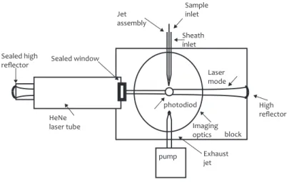
To meet the objectives 1, 2, 5 and 6 (Paragraph 1.2), two moni-toring campaigns were carried out with Osiris Environmental Dust Monitors (‘Osiris’ in short, see Annex 1). Hourly concen-trations of PM10 and PM2.5 were measured during two periods
of approximately one month each (during September/ October 2007 and March 2008). The Osiris is used because of its reproducibility, cost-efficiency and ease of installing the instrument at different locations during a field campaign. The reproducibility is optimised by a normalisation procedure carried out both before and after the measurement cam-paign (see Annex 1 for further details and estimation of the reproducibility).
The disadvantage of the Osiris is that the measurements are not conform or equivalent to the reference method (gravim-etry). Calibration to the reference method was not carried out because 1) we were more interested in (relative) differences than in absolute concentration levels and 2) available gravi-metric measurements from only one location would not yield additional information when evaluating differences between
locations. Furthermore, for assessing spatial variation, the reproducibility of the Osiris instruments is more important than measurement of absolute concentrations in accordance with the reference method. The data analyses are thus carried out based on the Osiris measurements, normalised to one reference Osiris level only. Therefore, the Osiris concentra-tions expressed as ‘µg/m3’ in this report should be regarded as ‘Osiris µg/m3’ rather than ‘reference µg/m3’. It is not
pos-sible to study absolute levels of PM concentrations and, for example, the fraction of PM2.5 /PM10.
The methods of data analysis are presented in Paragraph 2.5. To identify the influence of traffic, the monthly averaged concentration of NO 2 was measured by passive sampling at
the eleven locations. The Palmes tubes used for the measure-ments were supplied and analysed by Gradko Environmental (UK). The duration of a sampling period depends on the loca-tion. The sampling started on the day that the Osiris instru-ment was installed and ended on the day it was removed.
Mobile measurements 2.1.2
Besides the Osiris monitoring campaign carried out at the eleven locations, measurements were made throughout the studied area with a mobile unit. These measurements were used for objectives 3, 4 and 5 of the BOP programme (Para-graph 1.2).
With respect to the mobile measurements, the following questions were specifically formulated:
What is the representativeness of network measurement 1.
data within a city? In other words: to what extent are measurements, collected at a fixed urban background station, representative of the quality of the air in other background areas within the same city? This is referred to as the urban representativeness of a monitoring station. (objective 3)
Is it possible to quantify a scale length for which measured 2.
concentration data are representational? This is referred to as the local representativeness of measurements at a fixed location. (objective 4)
What are the changes in PM concentration levels meas-3.
ured when travelling through a city? More specifically, is it possible to estimate an (average) concentration gradient, that is, an absolute concentration change per kilometre? (objective 5)
The mobile measurements are complementary to the Osiris measurements at the fixed locations. A point measurement at a fixed location is representative of a small area around this point. Mobile measurements can be used to identify the
scale of this area, which is referred to as the local representa-tiveness (objective 4). Besides, in the Osiris set-up, to assess the spatial variability, results are in fact compared between those small areas. What is happening in-between the areas is PM10 GCN map for 2006. The monitoring locations from the Osiris campaign are represented by the dots and
numbers. 9 8 7 6 5 4 3 2 1 11 10 PM10 GCN map for 2006 PM10 concentration < 27 27 - 28 28 - 29 29 - 30 30 - 31 31 - 32 32 - 33 > 33 Locations Roads 1 Figure 4
PM10 GCN map for 2007. The monitoring locations from the Osiris campaign are represented by the dots and numbers. 9 8 7 6 5 4 3 2 1 11 10 PM10 GCN map for 2007 PM10 concentration < 27 27 - 28 28 - 29 29 - 30 30 - 31 31 - 32 32 - 33 > 33 Locations Roads 1 Figure 5
unknown, and for this the mobile measurements give addi-tional information.
Ten daytime periods between 27 September and 16 October were selected. The mobile unit that was used, contained high time-resolution equipment for on-line measuring of ambient levels of mass and particle numbers. The instruments used were a Laser Aerosol Spectrometer (LAS-x), a Condensation Particle Counter (CPC) and an Osiris. From the collected data PM10 and PM2.5 were calculated. The measurements were
taken while driving around different areas of Rotterdam, as well as from stationary positions, that is, near the Osiris locations. At different days, the LAS-x’ results were compared to the gravimetric TEOM-SES readings of the DCMR back-ground station at Schiedam. This was necessary to make a sound comparison between the TEOM data and the collected LAS-x data measured in other parts of the city. Further details about applied instruments and methods of data analysis are presented in Paragraphs 2.4 and 2.5.
GCN 1 x 1 km
2.2
2background
The large-scale concentration maps (GCN) provided yearly by the Netherlands Environmental Assessment Agency (PBL) serve as the background levels in local air-quality modelling. It is, therefore, important to assess the uncertainty in the GCN maps. The GCN maps are produced by calibrating OPS model calculations to measurements from the Dutch monitoring network (LML) (Velders et al., 2008). For PM10, the current
calibration procedure is to add the same value (14.4 µg/ m3) to the modelled concentration in each grid cell, in the Netherlands. The spatial resolution of the GCN maps is 1 x 1 km2. In 2006, the 5 x 5 km2 model grids were converted to 1 x
1 km2 grids, by interpolation. In 2007, the modelling
resolu-tion was enhanced to 1 x 1 km2 for most of the Dutch sources.
Shipping and foreign sources were still modelled at 5 x 5 km2
resolution. Consequently, the spatial variability near roads and industry hotspots increased. The PM10 GNC maps for 2006
and 2007 are presented in Figure 4 and Figure 5, along with the monitoring locations from the Osiris campaign. It is noted that the GCN map for 2007 was not yet available when the locations in this study were selected.
From Figure 4 and Figure 5, the difference between interpo-lating from 5 x 5 km2 (2006) and modelling at 1 x 1 km2 (2007)
is obvious. The 2006 presentation of the GCN concentrations is similar to the picture on the left in Figure 2, with increasing urban background towards the centre of the city. In 2007, the map is similar to the picture on the right in Figure 2, showing an urban area with more spatial variation in the background concentration. Also, the impact by urban motorways is visible on the GCN map, as the urban motorways around Rotterdam are situated in the GCN grid cells with highest concentrations. However, it should be noted that the range between the lowest en highest concentrations in both GCN maps is only 6 µg/m3. Within the area in which the urban monitoring locations are situated, the range is only 2 µg/m3, at the most. Spatial variability is, thus, very small in both maps.
The spatial variation in the urban PM10 background levels from
the GCN 2006 and 2007 maps is assessed and compared to the spatial variation derived from the measurement cam-paigns in September/October 2007 and March 2008. Since the GCN maps present average yearly concentrations, and both campaigns only cover one month each, the comparison is based on differences relative to the concentration levels. This is done by comparing the spatial coefficients of variation (see Paragraph 2.5).
Measurement locations
2.3
As mentioned in Paragraph 2.1, eleven monitoring locations in and around Rotterdam/Rijnmond were chosen and presented on a map in Figure 6. A description of the locations and objec-tives is given in Table 1.
The locations 2, 3, 4, 5 and 9 are regarded ‘true’ urban background stations for studying the variability of the urban background. The gradient from regional to urban background is studied from locations 6, 1 and 9. Location 6 is referred to as regional; it is not a rural site, since it is located close to the city of Delft in the north and close to the greenhouse area in the north-west. Location 9 is the DCMR urban background monitoring station at Schiedam, and actually lies in the vicinity of a heavy-traffic crossroad and the motorway A20, but is screened off from this traffic by some multi-storey buildings. The RIVM station Schiedamsevest (7) is characterised as an urban background station; it is located relatively close to the river ‘Nieuwe Maas’ and the harbour ‘Leuvehaven’. Therefore, inland shipping may influence the PM concentrations at this
Description of monitoring locations and specific objectives
Nr Monitoring location Monitoring objective Possible local influence
1 Schiedam Kethel, Educatief Centrum Regional to urban background
2 Schiedam West, Tennisvereniging Urban background
3 Rotterdam Nieuwe Westen, CBS Mozaiek Urban background
4 Rotterdam Provenierswijk, Hildegardis MAVO Urban background
5 Rotterdam Crooswijk, Speeltuinvereniging Urban background
6 Schipluiden, Zouteveensweg Regional background
7 Rotterdam city centre, RIVM Schiedamsevest Urban background Inland shipping
8 Vlaardingen, DCMR Vlaardingen Urban background Industry/harbour and urban traffic
9 Schiedam, DCMR Schiedam Urban background
10 Rotterdam Noord, Bentinckplein Traffic location
11 Rotterdam Overschie, DCMR Overschie Urban background Motorway traffic
location, at wind directions from south to east. Location 8 is influenced by traffic from the road that crosses the railway near the railway station at Vlaardingen. Influence from indus-try and harbour is expected when the wind direction is west to south. Location 10, at Bentinckplein, is a traffic station. The DCMR monitoring station at Overschie (11) is also character-ised as a traffic station; influence from motorway traffic (A13) is highest when the wind direction is west to south.
Mobile measurements
2.4
With respect to the mobile measurements, the experimental data presented here were collected with a (small) mobile unit. This unit contained high time-resolution equipment for on-line measuring of ambient levels of mass and particle numbers. The use of mobile laboratories has become a common feature (e.g. Seakins et al., 2002) but recording measurements ‘while driving’ is a rather new approach. During an extensive campaign, Bukowiecki et al. (2002; 2003) measured on-road concentrations of trace gases and various aerosol parameters in a mountainous Swiss area. In their studies, the suitability of the mobile-measurement approach for short- and long-term air-pollution investigations was shown. Another variant is the ‘real-world’ measurement of pollutants in exhaust emissions, produced by vehicles driving at a short distance ahead of the mobile laboratory (e.g. Kittelson et al., 2000; Canagaratna et al., 2004).
In our campaign, the mobile measurement technique was used along roads within the city of Rotterdam. Measured aerosol properties were restricted to mass (PM10 and PM2.5)
and particle number. The latter is used for the detection of influence from local traffic nearby, for which data were elimi-nated. The shortest length scale of interest here is that of an urban street (∼30 m). Even with the low vehicle traveling
speeds typical in urban agglomerations (∼30 km/h), param-eters need to be measured with high time resolutions (<20 s). Measurements were taken on ten days, between 27 Sep-tember and 16 October, with a mobile unit equipped with registrating measurement equipment, a GPS and a power generator. The measurements were carried out while driving, as well as when parked at certain locations.
For the campaign, three suitable routes were chosen. They are characterised as ‘regional to city centre’ (going from Schipluiden to Schiedamse Vest, and back), ‘urban’ (travel-ling past background locations within the urban centre) and a ‘gradient’ route from west to east and back (from Vlaardin-gen to Crooswijk). In Vlaardin-general, for all these routes, around 5 locations were visited twice a day; between these locations the shortest possible route was followed, following main roads. At the fixed locations, measurements close to the Osiris were carried out during 15 to 30 minutes. In Annex 8, a detailed scheme of the various routes is given.
For collecting the mobile measurements, different instru-ments for measuring size distribution and mass concentration of PM10 and PM2.5 were placed in the mobile unit. The
instru-ments used were a Laser Aerosol Spectrometer (LAS-x (see Annex 2) from PMS Inc.), a Condensation Particle Counter (CPC from TSI inc.) and an Osiris monitor. LAS-x and Osiris are optical instruments. In the campaign the LAS-x and Osiris were compared to a gravimetric instrument, the TEOM-SES of DCMR. The TEOM-SES was used for data analysis, with a standard correction factor of 1.3. This TEOM-SES was used for the comparison instead of FDMS, because most of the standard stations were equipped with the TEOM. In the ten days of measuring, there were no PM2.5 measurements by
TEOM-SES, so here only the FDMS was used. A description of Monitoring locations in Rotterdam/Rijnmond
9 8 7 6 5 4 3 2 1 11 10
Monitoring locations in Rotterdam/Rijnmond
Monitoring location Road type Highway Main road Other roads 1 N209 N470 N471 A4 A13 A20 Figure 6
the instruments is given in Annex 2. The comparison analysis is presented in Annex 3.
The weather conditions for the ten days of our mobile campaign are given in Annex 10, in which data on Rotterdam Airport (from the Royal Netherlands Meteorological Institute (KNMI)) are presented. On most of these days, wind speeds were relatively low, except for the first and last two days. During the campaign, wind direction was predominantly east or west. There was some rainfall on 1 and 3 October.
Data analysis
2.5
This paragraph describes the method of data analysis that was applied in the study. It starts with a description of the analysing method of the two month-long monitoring cam-paigns, at eleven locations, to assess spatial and temporal variability. Subsequently, the analysing methods are pre-sented that were used for the mobile measurements during specific days.
Osiris monitoring campaigns 2.5.1
The data analyses of the Osiris measurements from the eleven locations are applied after normalisation of the raw data to one reference Osiris level and outlier removal (see Annex 1). Annex 4 presents the normalisation factors.
Spatial variation
For the analysis of the spatial variation, first the locations were identified that represented real urban background locations during both the monitoring periods. This was done by assessing the differences in the mean concentration over both periods. Daily average concentrations of PM10 and PM2.5
were derived from the hourly data. Afterwards, the average concentration during both monitoring periods was caulated for each location , from the daily averages. Days were only taken into account if the daily average concentrations were available from all eleven locations. Due to power and instru-ment failure, there were several days without data, for some locations:
On certain days during the campaign in September/
October 2007, there were problems at locations 7 (Rotter-dam city centre) and 9 (Schie(Rotter-dam). As a result, there were only 16 days for which data were available from all eleven locations, during this campaign (3 to 18 October). During the campaign in March 2008, severe power prob-
lems were encountered at location 2 (Schiedam West). There were so few measurements available from this loca-tion that it was decided to exclude it. At localoca-tion 7 (Rot-terdam city centre), the Osiris instrument collapsed after 5 days of monitoring and, consequently, data were lost. And, since there were also two days without data from location 9 (Schiedam), the total number of days for which data were available from all eleven locations, during the second campaign, was 19 (12 to 17 March, 19 to 24 March, 26 March to1 April).
The uncertainty (1σ) in the mean concentration over the moni-toring period, per location, was estimated to be 10% for PM10
and 5% for PM2.5 (see Annex 1). This uncertainty refers to the
reproducibility (comparability between instruments). It does not include the bias towards reference concentration values. The mean concentration at each location was, subsequently, compared to the mean at the predefined urban background locations 2, 3, 4, 5 and 9. The differences (relative to the urban background mean) were plotted in column charts, allowing the identification of real urban background locations and hotspots.
Next, as a measure of spatial variability in urban background PM concentrations, the spatial coefficient of variation (SCV) was calculated. The SCV has been expressed as the standard deviation in measured concentrations divided by the mean measured concentration. The SCV was calculated, based on the locations identified as urban background locations. The SCV was calculated for the mean concentration per campaign. The uncertainty in the concentration per location was estimated at 10% and 5% for PM10 and PM2.5, respectively.
The SCV needs to be compared to the measurement uncer-tainty. If SCV values are higher than the uncertainty in the measurements, it can be concluded that the spatial variability was significant. If lower SCV values are found, no significant spatial variability can be determined. In other words, it was less than the measurement uncertainty. Since the uncertainty in the measurements itself is uncertain (it is an estimation), SCV values below the measurement uncertainty do not lead to the conclusion that the spatial variability is zero.
SCVs were calculated for the measurements during both monitoring campaigns and for the 2006 and 2007 GCN maps. A comparison was made between the spatial variability in the measurements and the GCN maps.
Regional to urban background gradient
The regional to urban background gradient analysis was done by wind rose analysis of the gradient between locations 6, 1 and 9, based on daily average concentrations. The gradients were calculated, based on linear regression,using the data from the three locations. This analysis was based on the above mentioned days used in the spatial analysis and on additional days for which the daily mean concentration was available from the locations 6, 1 and 9 (campaign 1: 21 to 29 September + 3 to 21 October 2007; campaign 2: 6 to 17 + 19 to 24 March + 26 March to 1 April 2008).
Temporal variability
A distinction has been made between the regional back-ground, urban background and traffic locations. Apart from the analysis of the temporal coefficient of variation (TCV), based on daily average concentrations (see explanation of SCV), the rate of change on an hourly temporal scale has been investigated.
Mobile measurements 2.5.2
For the mobile measurements, data analysis involved the LAS-x and CPC results. LAS-x data were converted into mass concentrations (PM10 and PM2.5). The CPC dataset consists of
corresponding particle number concentrations, and was used to detect the possible influence of traffic emissions nearby. High values of CPC numbers indicate the presence of vehicles.
When the particle number concentration deviated by more than 3 times the standard deviation, the corresponding LAS-x data were eliminated. This was done for measurements near the Osiris stations, as well as for the data obtained during driving. In addition to this, in the driving route analysis, data were only used when the mobile unit’s speed was above 5 km h-1 in order to avoid interference from traffic emissions during
stop-and-go situations (traffic lights, traffic jams). The unit’s speed was calculated from the GPS data.
To explore the urban representativeness of the Schiedam station (location 9), the (mobile) LAS-x data were compared to the TEOM-SES results obtained at this station. To do so, the LAS-x had to be scaled according to synchronised measure-ments from the TEOM at this station. The time resolution of the TEOM-data is one hour. The measurements with the LAS-x resulted in several periods of about 20 minutes on the Schie-dam location. Average LAS-x data were compared with inter-polated (hourly) TEOM data. For further details see Annex 3. In the gradient analysis, the changes in concentrations ‘while on the road’ were quantified by use of linear regression analysis. Subsequently, the change in the time variable was replaced by the distance covered An average estimate (per day) was then obtained by averaging the absolute results. When dealing with spatial concentration data in a geographi-cal context, identifying an appropriate sgeographi-cale for analysis is a critical issue. In this study, the mobile monitoring method was applied to collect spatially representative measure-ments of particulate matter (here only PM10 was considered).
A geostatistical technique (semivariogram) was applied to characterise the appropriate spatial-analysis scale as defined by the semivariogram range, the maximum distance of spatial dependence within the concentration data. Such a distance may be considered as the maximum distance for which measurements at a fixed location could still be used or would still be ‘representative’. This method was used to identify the area size, by characterising the degree of spatial autocorrela-tion in a dataset. Examples of this technique can be found in Lightowlers et al. (2008) and Larson et al. (2007). For more details see Annex 11.
3
Identification of urban background
3.1
locations based on Osiris data
Annex 5 presents the measured daily average PM concentra-tions at the eleven monitoring locaconcentra-tions, during both Osiris monitoring campaigns. For PM10, it also presents a
compari-son with TEOM-SES data from measurements by DCMR, simultaneously recorded at locations 9, 10 and 11. The ratios of the measurements collected by both instruments, differed between the locations. However, assuming that the relative uncertainty (1σ) in the mean concentration over the monitor-ing period of both the Osiris and TEOM-SES were in the order of 10% (see Annex 1 for Osiris), the differences found are within the uncertainty range. The performance of the Osiris instruments, therefore, cannot be evaluated by this compari-son. Annex 5 also presents the reference (gravimetric) PM measurements taken by RIVM at locations 9 and 10. Based on the regressions between Osiris and gravimetry, it can be con-cluded that the Osiris measurements have underestimated the PM concentrations. The underestimation during the first campaign was higher than during the second.
The meteorological variables, as measured by KNMI at Rot-terdam Airport, are presented in Annex 10. The prevailing winds during the first monitoring campaign were north-east. The monitoring period was characterised by high pressure systems and little precipitation. The temperature was mostly between 10 and 15 ºC, decreasing by the end of the monitor-ing period.
During the second monitoring campaign, there were few days with high PM concentrations compared to the first monitor-ing campaign. This can be explained by the large differences in weather conditions. Apart from lower temperatures, the wind direction was 180º different (south-west). Regional PM background concentrations are higher when air is being trans-ported over land rather than over sea. This explains the lower PM concentrations during the second monitoring campaign. Besides, March 2008 was a windy and wet month, causing enhanced dispersion and washout of aerosol particles. Annex 6 presents the measured NO2 concentration, indicating
the influence from traffic at the locations. The NO2
concentra-tions are shown to follow the same pattern in both monitor-ing periods. Traffic influences can be seen at locations 8, 10 and 11. During the second campaign, with westerly winds, the traffic influence at Overschie (location 11) was indeed higher than during the first campaign. In Vlaardingen (location 8)
and at Bentinckplein (location 10), the traffic influence did not seem to depend on the wind direction. It is also appar-ent, that the NO2 concentration was the lowest at regional
background locations.
An overview of the differences between the average meas-ured concentrations of PM2.5 and PM10 is presented,
allow-ing the identification of urban background locations. The first monitoring campaign is discussed first, followed by the second.
Figure 7 shows the difference between the location specific mean and the urban background mean PM concentration, relative to the urban background mean, for the first monitor-ing campaign. The urban background mean was derived from the predefined ‘true’ urban background stations 2, 3, 4, 5 and 9. Uncertainty intervals were based on the estimated repro-ducibility of 10% (PM10) and 5% (PM2.5) in the mean
concentra-tion over the monitoring period.
Figure 7 shows concentration differences, ranging from -14 to +13% for PM10 and from -15 to +22% for PM2.5.As can be seen
from the uncertainty intervals, only the largest differences are significant. Several aspects of Figure 7 are discussed:
Locations 6 and 10;
As could be expected, the lowest PM10
concentration was measured at the regional background location 6, while the highest PM10 concentration was
meas-ured at the traffic location 10, Bentinckplein. For PM2.5,
the concentrations were the second lowest and second highest. These results provide confidence in the reliability of the dataset.
Locations 2, 3, 4 and 5;
These locations are the ‘true’ urban
background stations and, as could be expected, had the lowest concentrations (besides the regional location 6 and location 1, which is situated at the edge of the city).
Location 9;
The concentration of PM10 (and to a lesser
extent PM2.5) was relatively high. It may be that, with
easterly winds, the impact of traffic from the nearby cross-roads and the motorway A20 was stronger than expected. However, this did not show up in the NO2 measurements. Locations 7 and 8;
These locations were urban background
stations, potentially influenced by local sources, such as inland shipping, harbour/industry and traffic. At location 7, as was expected in view of the prevailing easterly winds, no impact of shipping was measured for PM10 and PM2.5.
Hence, location 7 was regarded a ‘true’ urban background location during this monitoring period and has been incor-porated in the analysis of spatial variability (Paragraph 3.2).
The concentrations of PM10 and PM2.5 were relatively high
at location 8, which was attributed to the impact of traffic.
Locations 6, 1 and 9;
These locations were selected to
determine the gradient from the regional background to the urban background. From these three locations, the lowest PM10 and PM2.5 concentrations were measured at
location 6 and the highest concentrations were measured at location 9, as was . Therefore, the results may be suf-ficient for analysing this gradient.
Location 11;
Since the Overschie station is a ‘motorway station’ it is remarkable that both PM10 and PM2.5
con-centrations were low (for PM2.5 even lower than regional
background). In view of the potential influence of the A13 motorway near to station, this was unexpected. Indeed,
the NO2 measurements indicated influence from traffic,
even though the prevailing winds were easterly (see Annex 10). From the comparison with TEOM-SES data (Annex 5), it is not possible to conclude whether the Osiris instrument at location 11 has functioned inadequately. In view of this uncertainty, the data from location 11 were not used in further data analyses.
Figure 8 shows the difference between the location specific mean and the urban background mean PMconcentration, relative to the urban background mean, during the second campaign. The urban background mean was derived from the predefined ‘true’ urban background stations 3, 4, 5 and 9. Difference between the location specific mean and the urban background mean PM concentration, relative to the
urban background mean, during the first monitoring campaign (%). Here, the urban background mean is the mean at locations 2, 3, 4, 5, and 9. 1 2 3 4 5 6 7 8 9 10 11 location number -30-25 -20 -15 -10 -5 0 5 10 15 20 25 3035 40 % PM 10 PM2.5 Uncertainty
First monitoring campaign
PM concentration difference Figure 7
Difference between the location specific mean and the urban background mean PM concentration, relative to the urban background mean, during the second monitoring campaign (%). Here, the urban background mean is the mean at locations 3, 4, 5, and 9.
1 2 3 4 5 6 7 8 9 10 11 location number -30-25 -20 -15 -10 -5 0 5 10 15 20 25 3035 40 % PM 10 PM2.5 Uncertainty
Second monitoring campaign
From a comparison between Figure 8 and the results from the first monitoring campaign in Figure 7, is concluded that the range of variability of the concentrations between the loca-tions during the second campaign was far smaller than during the first, both for PM10 and PM2.5. Also, the overall levels of
PM were lower during the second campaign. The latter was against expectations as during the winter period higher con-centrations were expected due to less favourable dispersion conditions compared to during the first monitoring campaign. However, the wind direction was mainly south-west with relatively high wind speeds, while during the first campaign easterly winds dominated. In fact, meteorological conditions were reversed, compared to what was expected during the set-up of the monitoring strategy. The prevailing winds during this month were representative of a large part of an average year in the Netherlands. In this respect, the campaign has been very useful.
Both PM10 and PM2.5 concentration differences ranged from -8
to +10 %. Taking the measurement uncertainty into account, those differences are not significant. Main aspects to discuss are:
Location 5;
The PM10 concentration at this urban
back-ground location was high, compared to the other urban background locations. During the campaign, construction activities took place at the cemetery, located to the north-east. However, the wind from that direction was very light, so it is unlikely that the activities influenced the measure-ment. Therefore, location 5 was retained in the PM10 data
analyses.
Location 7; No influence from shipping was seen. Location
7 was regarded as a ‘true’ background location during this period and has been incorporated in the analysis of spatial variability (Paragraph 3.2).
Location 8
; Typically, the PM10 concentration was in the
lower range, while the PM2.5 concentration was in the
higher range. The low PM10 concentration is puzzling,
espe-cially since the NO2 measurements indicated a high traffic
contribution. Under the westerly wind circumstances, influence would be expected from harbour and industrial activities. It may be that the influence of the harbour and industrial activities were restricted to the finer fraction of PM (due to combustion processes). Care must be taken, however, because the differences are small compared to the measurement uncertainty.
Location 11
; The motorway station situated on the east side of the motorway A13, had a higher ranking compared to the first campaign. Due to the south-west wind direction, the impact of the motorway was indeed expected to be higher during the second campaign.
Spatial variability in urban background
3.2
The spatial variability in urban background PM concentra-tions is measured by the spatial coefficient of variation (SCV). The SCV is expressed as the standard deviation in measured concentrations divided by the mean measured concentration. Locations representing the urban background monitoring stations were: 2 (only available during the first monitoring campaign), 3, 4, 5, 7 and 9. Table 2 presents the SCV values for PM10 and PM2.5, based on the mean concentration at the
mentioned locations during the monitoring periods. The SCV values were lower than the measurement uncer-tainty (1σ), which was estimated at 10% for PM10 and 5% for
PM2.5. It must be concluded that, during both monitoring
cam-paigns, no significant spatial variability could be determined in the period’s mean concentration at the urban background locations.
Also, a single-factor ANOVA analysis, based on daily average PM10 concentrations at the urban background locations during
the first monitoring campaign, indicated that the spatial vari-ation was not significant (p>0.05). This means that the spatial variation was far less than the temporal variation from day to day (see also Paragraph 3.6).
Under conditions that favour high PM concentrations (such as during the first monitoring campaign in September), the spatial variability in the urban background concentration of PM2.5 was less than for PM10. Local sources of PM10, such as
non-exhaust emissions from traffic and construction activi-ties, may account for this.
To put the calculated urban background PM10 variability in
per-spective, the variability in GCN maps was assessed for com-parison. Keeping in mind that GCN maps are yearly averages and the monitoring campaigns only covered one month each, calculating SCV values allowed a normalised comparison. The GCN concentrations for the 1 x 1 km2 grid in which the
monitoring locations were located are presented in Annex 7. The concentrations at locations 2, 3, 4, 5, 7 and 9 were used to determine the SCV in the urban background. The calculated SCVs for both monitoring campaigns, GCN 2006 and GCN 2007, are presented in Table 3.
The low SCV values from the GCN reflect the lack of spatial variation in PM, due to long-range transport.
The spatial variability is lower in the GCN maps than in the measurements. The higher, measured SCV values do not automatically mean that the spatial variability was larger than
Measured spatial variability of urban background PM concentration
PM10 PM2.5
Monitoring campaign locations n SCV (%) locations n SCV (%)
1 (September/October 2007) 2,3,4,5,7,9 6 9.3 2,3,4,5,7,9 6 3.9
2 (March 2008) 3,4,5,7,9 5 4.3 3,4,5,7,9 5 4.6
Spatial coefficients of variation (SCV) in the PM urban background based on the average concentration at the locations over the monitoring periods.
would be expected from the GCN data. Due to the measure-ment uncertainty, one may only conclude that the spatial vari-ability of PM10 was smaller than the measurement uncertainty.
In fact, the uncertainty in the GCN concentrations is estimated at 15% (Velders et al., 2008), indicating that the variability of 2% is not significant.
The question now is: how well do the monitoring locations represent the 1 x 1 km2 grid cells of the GCN? One may expect,
in view of the relatively low spatial variability in the urban background cells, that within a grid cell the variability would be low, as well. Hence, a monitoring station located at a suf-ficient distance from local sources (no more than 2500 motor vehicles per day within a radius of 50 meter; Larssen, 1999) would be representative of the urban background concentra-tion within a 1 x 1 km2 grid cell. One of the goals of the mobile
measurement campaign, related to this question, was to assess the spatial representational scale around the measure-ment locations. (see Paragraph 3.4).
Urban representativeness of a measurement station
3.3
The first question with respect to the mobile measurements was if point measurements of PM10 and PM2.5 at an urban
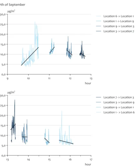
background station were comparable with average levels measured in other parts of the city (complying with the definition of urban background). Location 9 in Schiedam is the official DCMR background station at which PM is meas-ured with TEOM instruments (see Annex 40). To investigate the representativeness of this station for other background locations, LAS-x measurements were first levelled with the TEOM readings by using the factors determined in Annex 40 (see the Annex for more details). Also, any possible influence of traffic was considered and if necessary, affected data were removed. The resulting time series were compared with the corresponding time series of the TEOMs from this location. Figure 9 gives three examples of such time series. These were registrated with the LAS-x and TEOM equipment, on 27 Sep-tember, 4 and 11 October.. The LAS-x data points represent averages over the stationary, as well as the ‘mobile’ measure-ment periods. The first point in the LAS-x graph is always a measurement at a fixed location. On 27 September, the route which was driven was from Schiedam Kethel (location 1) to the city centre of Rotterdam (Schiedamsevest, location 7) and back. The west-to-east route on 4 October from Vlaardingen (location 8) to Crooswijk (location 5), was driven twice. This was also the case for the north-to-south route on 11 October, from Overschie (location 11) to Schiedamsevest (location 7). The figures for the remaining days are given in Annex 6.
Visual inspection learned that the LAS-x recordings (to some extent) resembled the hourly variation observed at Schiedam, for both PM10 and PM2.5. The TEOM variation appeared quite
considerable: changes in the order of 20 µg/m3 or more were observed within a timeframe of a few hours. This pattern was only partially followed by the LAS-x. The LAS-x series further possessed a variation in time that was smaller in magni-tude and higher in frequency, due to the shorter averaging time intervals revealing local influences. An example is the relatively large difference for PM10 (and less for PM2.5) found
on 27 September around 13:30 hrs (route from location 7 to location 3). This was caused by road construction, resulting in more resuspended dust and many traffic jams. This route was, therefore, not representative of the urban background. The above findings appear applicable to most recorded measurements. In general, the hourly variation measured at Schiedam was recognisable in the LAS-x measurements, sup-porting the idea of a large-scale ‘blanket’ of PM lying over the entire city, with variations caused by both regional transport of PM and weather conditions. However, large deviations occurred within some of the series, which could have been due to local influences on the LAS-x measurements.
Table 4 gives the average difference in concentrations between LAS-x and TEOM-SES (in case of PM10) and
TEOM-FDMS (PM2.5) measurements, for each day. These are
pre-sented, separately, for the mobile and stationary measuring periods, as well as for both modes together. A positive sign means that the LAS-x measured a higher (average) concentra-tion than the TEOM at Schiedam.
Averaged over all measurements days, the difference for PM10 was -1.5 µg/m3, and for PM2.5 -1.9 µg m-3. On most of the
days (8 out of 10) the (average) absolute difference between the LAS-x and TEOM time series at Schiedam was less than 5 µg/m3. On the remaining two days (15 and 16 October)
rather large differences were found which appear systematic throughout both days (see Annex 9). A possible explanation would be that on these days no representative calibration factor for the TEOM was determined. Instead, the average value was used. It may well be that this average is not repre-sentative of these two particular days. However, studying the weather conditions for these days, no apparent explanation was found.
In terms of percentages, the daily differences measured for PM10 were between -36% and +26%. Without 15 and 16 October,
the range would become -24% to +17%. Taking into account that 1) the direct influence of vehicular emissions could still have been present in the dataset and 2) measurements
Spatial variability of urban background PM10 for measurements and GCN
Measurement / GCN map n SCV (%)
Monitoring campaign 1 6 9.3
Monitoring campaign 2 5 4.3
GCN 2006 6 1.2
GCN 2007 6 1.8
Spatial coefficients of variation (SCV) in the urban background concentrations for both monitoring campaigns and GCN.