Approximate Sequence Alignment using the Bidirectional FM-index

(1)

Bidirectional FM-index

Approximate Sequence Alignment using the

Academic year 2019-2020

Master of Science in Computer Science Engineering

Master's dissertation submitted in order to obtain the academic degree of

Counsellor: Dr. Dries Decap

Supervisor: Prof. dr. ir. Jan Fostier

Student number: 01503824

(2)

(3)

Bidirectional FM-index

Approximate Sequence Alignment using the

Academic year 2019-2020

Master of Science in Computer Science Engineering

Master's dissertation submitted in order to obtain the academic degree of

Counsellor: Dr. Dries Decap

Supervisor: Prof. dr. ir. Jan Fostier

Student number: 01503824

(4)

PERMISSION OF USE ON LOAN I

Permission of Use on Loan

"The author gives permission to make this master dissertation available for consultation and to copy parts of this master dissertation for personal use.

In all cases of other use, the copyright terms have to be respected, in particular with regard to the obligation to state explicitly the source when quoting results from this master dissertation."

Luca Renders Ghent, May 2020

(5)

ACKNOWLEDGMENTS II

Acknowledgments

Five years ago, I started my engineering studies with the goal of becoming an expert in chemical technology. Now, I am finalizing my studies in Computer Science Engineering and completed a thesis that is applicable to bioinformatics. Oh how the times have changed. I could not have done this without the help of so many people during these past five years.

First and foremost, I would like to express my gratitude to my supervisor prof. dr. ir. Jan Fos-tier, for offering me the chance to work on this interesting project, for his enthusiasm and for opening my view to this fascinating interdisciplinary field of research. The brainstorming and feedback sessions, both on-campus and online due to the coronavirus, helped me a great deal in achieving the best possible dissertation. I also want to thank my counsellor dr. Dries Decap for his feedback throughout the year.

Second, I would like to thank my family for the never-ending support. I am also grateful for the friends I have made during my studies. They have been a continuous source of joy and entertainment, which was more than emphasized during the lockdown.

Lastly, Ina, I would like to thank you for always being there for me and for always listening to my, sometimes incohesive, ramblings about my thesis and computer science in general.

Luca Renders Ghent, May 2020

(6)

ABSTRACT III

Abstract

With the advent of High-Throughput Sequencing methods, the accumulated volume of sequenc-ing data grows faster and faster. Advancements in computer architecture are insufficient to keep up with the ever growing database of sequences. As a result, the there is an urgent need for efficient data structures and algorithms to analyze sequencing data. In this dissertation, we analyze how lossless approximate sequence alignment, where substitutions, insertions and deletions are allowed, can be improved. To answer this question, we propose a number of im-provements on approximate pattern matching algorithms using a bidirectional FM-index, as well as on the recently introduced concept of search schemes. The inherent redundancy associated with the edit distance metric is analyzed. The performance of the different search schemes and the effects of the improvements are studied by aligning artificial reads to the human genome. Our results showed that efficiently implementing a search schemes has a larger effect than choosing the optimal search scheme. Nonetheless, some schemes perform better than others on average. The results were compared to SeqAn v3, a publicly available library that imple-ments search schemes. We found that our implementation surpasses the results achieved by SeqAn v3.

(7)

Approximate Sequence Alignment using the Bidirectional

FM-index

Luca Renders

Supervisor: Prof. dr. ir. J. Fostier Counsellor: Dr. D. Decap Abstract—With the advent of High-Throughput Sequencing methods, the

accumu-lated volume of sequencing data grows faster and faster. Advancements in computer architecture are insufficient to keep up with the ever growing database of sequences. As a result, the there is an urgent need for efficient data structures and algorithms to analyze sequencing data. In this dissertation, we analyze how lossless approximate sequence alignment, where substitutions, insertions and deletions are allowed, can be improved. To answer this question, we propose a number of improvements on ap-proximate pattern matching algorithms using a bidirectional FM-index, as well as on the recently introduced concept of search schemes. The performance of the different search schemes and the effects of the improvements are studied by aligning artificial reads to the human genome. Our results showed that efficiently implementing a search schemes has a larger effect than choosing the optimal search scheme. Nonetheless, some schemes perform better than others on average. The results were compared to SeqAn v3, a publicly available library that implements search schemes. We found that our implementation surpasses the results achieved by SeqAn v3.

Keywords— Approximate Sequence Matching, Bidirectional FM-index, Search Schemes

I. INTRODUCTION

A

PPROXIMATE string matching is a well-studied problem in com-puter science. Commercial spell checkers have been around since the 1970s [1]. After Frederick Sanger determined the sequence of in-sulin in the early 1950s [2] and protein sequences became available, the need for automated sequence alignment in molecular biology arose and sequence alignment algorithms became central to bioinformatics applications.

In 2003, the human genome project was completed and for the first time, the DNA sequence of a human individual was established. This project took 13 years and cost over 3 billion USD. Today, the genome of any human can be sequenced for under a 1000 USD (see figure 1). High-Throughput Sequencing methods allow for cheap and parallel se-quencing of DNA, however, they fragment the DNA into millions of reads with no information on how they fit together. Among many other applications, this is where approximate pattern matching comes into play.

Fig. 1: Comparing the cost per human genome to Moore’s Law [3]. Formally, given a query pattern P (e.g. a read) and a search text T (e.g. a reference genome or a database of genomes), the basic task is to identify occurrences of P in T . If no errors are allowed, the problem is called exact pattern matching. Due to the presence of sequencing errors and natural variation (human individuals share roughly 99.9% of their DNA), one is often interested in finding occurrences of P in T within a certain Hamming distance (allowing only substitutions) or

Levenshtein/edit distance (allowing substitutions, insertions and dele-tions). This is called approximate pattern matching. As most practi-cal bioinformatics applications perform many queries for a given static search text T , the focus of this thesis is on approximate pattern match-ing usmatch-ing a full-text index.

Most bioinformatics tools (e.g. BLAT, BLAST, BWA, etc.) use lossy approximate pattern matching algorithms: they rely on heuristics to quickly identify some (but not necessarily all) approximate matches of P in T . By sacrificing some sensitivity, significant gains in perfor-mance can be obtained. This loss of sensitivity can manifest itself in many ways, for example, reads can be over-confidently mapped to the wrong position in genome, causing false-positive germline or somatic variants to be called. In contrast, in this thesis, the focus is on lossless algorithms that are guaranteed to retrieve all approximate matches of P in T .

In 2000, a new substring index, the FM-index, was proposed [4]. This index still allows for the alignment of sequences to a reference text in linear time of the pattern’s length, while having the benefit of being a very succinct (i.e. memory-friendly) data structure. In 2009, Lam et al. extended the unidirectional FM-index to a bidirectional FM-index. Using a bidirectional FM-index, patterns can be matched either from left to right, or from right to left. Curiously, this additional functionality opens up new possibilities for faster approximate matching [5].

In 2015, Kucherov et al. introduced the concept of search schemes. Informally, search schemes define how a pattern P is matched using a bidirectional index such that unsuccessful branches of the search tree are discarded as quickly as possible and runtime is minimized [6].

II. FM-INDEX

The FM-index a substring index proposed by Ferragina and Manzini in 2000 [4]. It is based on the Burrows-Wheeler transform [7].

Using conventional notation on strings, the Burrows-Wheeler trans-formation BWT(T) of a text T of size n that ends with a unique (and lexicographically smallest) sentinel character $ is defined as:

BWT(S)[i] = (

S[SA(S)[i]]− 1] if SA(S)[i] > 0

$ otherwise

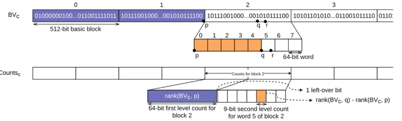
Here, SA(T) denotes the suffix array, an array over integer values that indicate the starting positions of the suffixes of T in lexico-graphical order. We need support for Occ[c, i] queries on the BWT that return the number of occurrences of character c in the prefix of BWT(T)[0, i)_{. One possible way to realize this, is through |Σ|} bit-vectors with constant-time rank support, e.g. using the rank9 algo-rithm [8]. Here, |Σ| denotes the size of the alphabet (e.g.|Σ| = 4) for DNA sequences). Exact pattern matching is then performed by match-ing character by character, from right to left. Let [i, j) denote the range over the suffix array for which the corresponding suffixes have P as a prefix. The range over the suffic array [i0_{, j}0₎_{whose suffixes have cP as} a prefix can then be computed by i0_{= C[c]+Occ[c, i}_{−1]+1 and j}0₌ C(c)+Occ[c, j_{−1]+1. Here, C[c] denotes the number of characters in} BWT(T)strictly smaller than c. These are pre-computed and stored in a small array of size |Σ|. Assuming Occ[c, i] queries can be performed in constant time, exact matching of a pattern P of size m takes O(m)

(8)

time. The size of the obtained range [i, j) denotes the number of occur-rences of P in T . The actual positions of the occuroccur-rences in T can be obtained using the suffix array. Often, only a subset of the suffixarray’s elements are stored: either every kth index of SA(T), or every kth suf-fix is stored. The latter has an improved worst-case running time but requires an auxiliary bit-vector with rank support to indicate the pres-ence or abspres-ence of index positions and to compute their offsets within the sparse SA. The full-text index that comprises a BWT representation and auxiliary tables is called the FM-index and may occupy as little as 2-4 bits of memory per character for DNA sequences.

A bidirectional FM-index is realized by also storing BWT(T0₎_the Burrows-Wheeler transformation of T0_{, the reverse of T . By keeping} track of both the range [i, j) over BWT(T) as well as the range [i0_{, j}0₎ over BWT(T0₎_{in a synchronized manner [5], one can extend a pattern} P to both cP as well as P c. By replacing the Occ data structure with a Prefix-Occ, this can be realized in constant time [9].

III. APPROXIMATEPATTERNMATCHING

Patterns do not necessarily have an exact match in a reference genome, either due to sequencing errors or genetic variation. Genetic variation is most commonly expressed as single nucleotide polymor-phisms (SNPs) [10]. Sequencing errors also result mostly in substitu-tions, deletions or insertions [11] w.r.t. the sequenced genome. The Il-lumina platforms suffer almost exclusively from substitutions whereas for Pacific Biosciences and Oxford Nanopore platforms, insertions and deletions are the dominant type of error. For this reason, it is inter-esting to consider approximate matches of a pattern (e.g. a read). Ap-proximate pattern matching thus involves identifying all occurrences of a query pattern P with respect to some distance metric. Usually, the Hamming distance (only substitutions) or Levenshtein/edit distance (indels and substitutions) are used. As mentioned in the introduction, we focus exclusively on lossless approximate pattern matching algo-rithms, where one has the guarantee that all occurrences of P are re-trieved.

The edit distance ED(X, Y), of two strings X and Y of length m and n, respectively, is defined by the smallest number of substitutions, insertions and deletions needed to transform X into Y .

Due to the recursive definition of the edit distance, it can be easily calculated using a dynamic programming algorithm. which uses an (m + 1)_{× (n + 1) alignment matrix AM, thus the memory complexity} is O(mn). Each cell takes constant time to compute, hence the time complexity is O(mn) as well.

A. Approximate Pattern Matching in the FM-Index

The goal is to find all (if any) occurrences of a pattern (e.g. a read) P in a text (e.g. a reference genome) T with at most K errors, i.e., we want to identify all infixes O of T for which ED(P, O) ≤ K.

The core idea is to explore all branches of the substring index until either an occurrence is found or until the maximum number of edit operations is exceeded. This is often referred to as ‘backtracking’. However, this naive search procedure quickly becomes computation-ally intractable for a larger number of allowed errors. Thus, most ap-proximate pattern matching tools only attain a feasible running time for a small number of errors (typically up to 4 errors are allowed [12]), or they rely on lossy approximate pattern matching algorithms that are not guaranteed to identify all occurrences of P in T .

A.1 Redundancy

The naive approach suffers from inherent redundancy associated with the edit distance metric: a single occurrence of a pattern P in T may be realized through multiple alignments with slightly different starting/ending positions in T .

In the search tree this entails that if a branch B reports occurrences (ED(B, P) ≤ K) , additional redundant branches Br_{might also report} occurrences.

A redundant alignment between P and B will have trailing or lead-ing gaps in either of the sequences. Four types of redundancy can be identified: adding leading characters to B, removing leading char-acters from B, adding trailing charchar-acters to B and removing trailing characters to B. The naive backtracking algorithm can be improved to eliminate these types of redundacny, which can significantly impact the search space (see section VI.

IV. SEARCHSCHEMES

Consider the human genome as a string over a 4-letter alphabet Σ_{= {A, C, G, T}. Assume the bases are randomly and uniformly} distributed over the genome. As the human genome has roughly 3 000 000 000 bases the expected number of occurrences of a 15-mer in the human genome under this assumption is greater than 1 (415_{< 3 000 000 000).}

For this reason, the search tree is highly dense in the neighborhood of the root, as all nodes in this neighborhood will have an expected number of 4 children.

Lam et. al were the first to note that due to this high density, most branches visited in the search tree will prove unsuccessful [5]. They proposed a scheme in which first part of a pattern P is exactly matched, thus going deeper into the tree and perform the approximate matching procedure on a less dense subtree of the search tree.

Kucherov et al. generalized this idea and defined the concept of search schemes [6]. Pockrandt adjusted the original definition by Kucherov et al. to be less restrictive [12].

Suppose a pattern P is partitioned into p parts. Each part Pi cor-responds to an infix of P , where if Pi = INm,n(P), then Pi+1 = INn,q(P)with 0 ≤ m < n < q ≤ |P |. A search S = (π, L, U) is a triplet of strings. π is a permutation string of length p over 1, 2, . . . , p, indicating the order in which the parts are searched. L[i] and U[i] give lower and upper bounds for the cumulative number of errors in all parts up to and including part Pπ[i], for 0 ≤ i < p. An error pattern is an integer string A of length p, where A[i] equals the number of errors in Pπ[i]. The weight k of string A equalsPp−1i=0A[i]. An error pattern A is covered by a search S = (π, L, U) if L[i] ≤Pi

j=0A[π[j]]≤ U[i], with 0 ≤ i < p. A K-mismatch scheme S is a set of searches for which each possible error possible error pattern A with weight k ≤ K is covered by at least one search.

Several search schemes have been proposed and these are analyzed for their performance in this thesis. They include the Pigeon H. S. [13], 01*0 seeds [14], schemes by Kucherov [6], schemes by Kianfar [9] and ManBest[12].

V. IMPROVEMENTS

A. Interleaved Bit Vectors

During the approximate matching procedure the number of occur-rences for each character in the alphabet before a certain index are cal-culated sequentially. This has up to 2 × |Σ| cache misses. By interleav-ing the rank9 bitvectors, one can reduce these cache misses, which can greatly reduce the running time.

B. Switch to Exact Matching

If at any point during the approximate matching procedure of a pat-tern P to an index I with a maximal edit distance of K, the minimal value of a row of the alignment matrix is K, then the only possible ap-proximate occurrences of the whole pattern to the current branch have trailing exact matches.

Exact matching is more efficient than approximate matching. For this reason, it is more efficient to switch to exact matching when for a node (d, [b, e)), minjAM[d, j] = K. Consider the case of backward search, as in the standard unidirectional FM-Index, and call the associ-ated prefix of n Pn. The exact matching procedure is then executed for every prefix of P, PREk(P), for which ED(Pn, SUFk(P)) = K 2

(9)

Assume banded alignment is used, in the worst case scenario AM[d, j] = K, _{for all j for which d − K ≤ j ≤ d + K and 2K + 1} exact matching procedures require to be performed. However, unless both the pattern and the branch have a long repeat of the same charac-ter, most of the started exact matching procedures will terminate early. In most cases, the number of exact matching procedures required will be limited and little overhead is introduced.

This improvement can also be applied to a search within a search scheme. Take a search S = (π, L, U) for which U[i] = U[i + 1] = e. If one of the reported occurrences of approximate matching procedure for the piece at π[i] has edit distance e, then piece π[i + 1] must be matched exactly if the pattern is an approximate match covered by search S. In this way, schemes can bypass the approximate matching procedure for the relevant piece and immediately start an exact match-ing procedure. The alignment matrix does not need to be created. C. Redundancy in between Parts of a Search

As searches of search schemes align a pattern P piece by piece, a cer-tain degree of redundancy inherent to the use of the edit distance metric might occur. If all occurrences of one piece Pπ[i]with an edit distance lower than or equal to some maximal value K are reported, then the search will start an alignment procedure for Pπ[i+1] for each occur-rence. Because of the redundancy as explained in section III-A.1, the alignment procedure will then be started for multiple, redundant occur-rences. Filtering this redundancy can significantly impact the running time.

To reduce this redundancy the new concept of clusters is introduced: A cluster {s, c, e} (s ≤ c < e) corresponds to part of a column j of the alignment matrix, i.e., all elements AM[i, j] with s ≤ i < e for which it holds that AM[i, j] = AM[c, j] + |c − i|.

AM[s, j], AM[c, j] and AM[e, j] are called the start, center and end of the cluster, respectively. The minimum value of the cluster is found at AM[c, j].

A cell AM[i, j] can be a part of multiple clusters. A cluster {c, c, c + 1} contains just one cell. Each cell AM[i, j] is part of at least one cluster.

Lemma V.1: Consider the optimal alignments of string X to string Y. For each optimal alignment that passes through one or more cells of cluster {s, c, e} and does not pass through the center, an equivalent alignment exists which passes through the center.

Proof: First, consider the case where an optimal alignment passes through cell AM[i, j], with s ≤ i < c. Because of the definition of a cluster, it holds that AM[i, j] = AM[c, j] + (c − i). Assume that AM[c, k]is leftmost cell on row c through which this optimal alignment passes. The optimal alignment path between matrix cells AM[i, j] and AM[c, k]_{entails exactly (k −j)−(c−i) gaps. Therefore, AM[c, k] ≥} AM[i, j] + (k−j)−(c−i) and hence, AM[c, k] ≥ AM[c, j]+(k −j). Therefore, an alternative alignment can be found for which the path in the alignment matrix runs from the origin to AM[c, j]; from AM[c, j] to AM[c, k]and then to the bottom-right element in an identical manner as the original path.

Second, consider the case where an optimal alignment passes through cell AM[i, j], with c < i < e and which does not go through AM[c, j]. Because of the definition of a cluster, it holds that AM[i, j] = AM[c, j] + (i_{− c). The value AM[i, j] can thus always} originate from AM[c, j] through a vertical path, as the difference in rows between these two cells is exactly (i − c).

As search schemes split the alignment in different stages, the con-cept of clusters provides an opportunity. Instead of reporting all ap-proximate matches of a piece smaller than or equal to a maximal edit distance K, one could opt to report only those matches that are also the center of a cluster. As each alignment that goes through cells of a clus-ter that are not the cenclus-ter can be replaced by an equivalent alignment that goes through the cluster center, no correctness is lost.

Checking if a node ends the alignment on a cell that is the center

of a cluster is simple. If a cell is the center, neither its parent nor one of its children can have a better alignment. If the search is depth-first, the value of the parent is always known when visiting the children. The values of all children are known when the search backtracks to the parent, so at this time it can be evaluated if the current parent is a cluster center and thus if it should report.

D. Caching and Reusing Parts of a Search Scheme

Many search schemes have multiple searches for which e.g. π[0], U [0]and L[0] are identical. Instead of recalculating the correspond-ing partial matches multiple times, they are cached and reused across different searches.

VI. EXPERIMENTS& RESULTS

The bidirectional FM-index as well as the search schemes are im-plemented in a C++11 stand-alone application that is available on GitHub1_.

A. Metrics

To compare different implementations where patterns P are approx-imately matched to a reference text T , different metrics are used. The most obvious metric is of course the running time of the approximate matching procedure. However, the running time metric can be influ-enced by the quality of the implementation. To compare to procedures on an algorithmic level, three other metrics are introduced:

Number of nodes visited: Approximate matching using the FM-index traverses a search tree in that FM-index. The number of visited nodes is an indication for the complexity and efficiency of an algorithm. Number of matrix elements filled in: To align a pattern P to a text T an alignment matrix is used. The matrix is reused for different branches of the search tree. At each node in the search tree a number of matrix elements will be filled in and thus calculated. This number will vary for the different search schemes. For exact matching, no matrix elements need to be calculated. Number of unique matches over number of reported matches: Different searches within a search scheme could return the same occurrence. Also, because of the inherent redundancy associated with the edit distance metric, some redundant matches might be found.

B. Dataset

To compare the different strategies, reads were aligned to the hu-man genome (GRCh38) [15]. All non-ACGT characters (e.g. Ns) of the reference genome were replaced by a randomly chosen nucleotide from {A, C, G, T}. All chromosomes were concatenated into a single string. It is possible that a read will be mapped across the boundary of adjacent chromosomes. However, it is possible to remove these occur-rences during post-processing, just as occuroccur-rences that wrap around the sentinel character can be removed.

As the reference text now only contains ACGT characters, the inter-leaved bit vectors from section V can be used. From the adjusted refer-ence genome, 100 000 reads of respectively length 250 bp and 100 bp were sampled. For each K ∈ {1, 2, 3, 4}, new sets of reads were gen-erated by introducing exactly K errors, with an equal probability for an insertion, deletion or substitution. By deleting or inserting a character, the length of the read might change, so that the smallest possible read is respectively 96 bp and 246 bp and the longest is respectively 104 bp and 254 bp long.

These reads are probably not very realistic, however they allow for comparing the performance of the different implementations.

C. Results

The results were achieved on a single core of 24-core AMD EPYC 7471 CPU running at a base clock frequency of 3.1 GHz. Running

1_{https://github.com/lurenders/Bidirectional-FM-index}

(10)

K = 0, |R| = 250

time avg. nodes avg. matrix el. avg. R/U

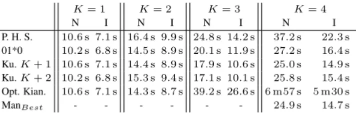
All strategies 4.0 s 250.00 0.00 1.00 K = 1, |R| = 250 Pigeon H. S. 7.1 s 324.86 192.26 1.03 01*0 6.8 s 340.09 214.30 1.03 Kucherov K + 1 7.1 s 324.86 192.26 1.03 Kucherov K + 2 6.8 s 340.09 214.30 1.03 Opt. Kianfar 7.1 s 324.86 192.26 1.03 Impr. Backtrack. 47.0 s 3429.76 10 282.93 1.01 Naive Backtrack. 1 m43 s 3937.72 11 804.73 1.05 K = 2, |R| = 250 Pigeon H. S. 9.9 s 476.76 805.49 1.42 01*0 8.9 s 463.53 595.61 1.34 Kucherov K + 1 8.9 s 425.92 536.30 1.20 Kucherov K + 2 9.4 s 488.23 551.88 1.35 Opt. Kianfar 8.7 s 414.55 498.52 1.07 Impr. Backtrack. 16 m8 s 67 865.24 339 294.43 1.02 Naive Backtrack. 20 m41 s 80 793.50 403 932.22 1.12 K = 3, |R| = 250 Pigeon H. S. 14.2 s 753.66 2075.66 1.81 01*0 11.9 s 640.43 1330.90 1.63 Kucherov K + 1 10.6 s 513.44 910.73 1.29 Kucherov K + 2 10.1 s 535.73 843.60 1.25 Opt. Kianfar 26.6 s 1789.13 1436.86 1.35 Impr. Backtrack. ∼4 h 30 m DNF DNF DNF Naive Backtrack. ∼5 h 20 m DNF DNF DNF K = 4, |R| = 250 Pigeon H. S. 22.3 s 1330.94 4950.71 2.28 01*0 16.4 s 968.12 2826.91 2.02 Kucherov K + 1 14.9 s 882.04 2046.91 1.87 Kucherov K + 2 15.4 s 981.93 1984.65 1.91 Opt. Kianfar 5 m30 s 28 417.93 18 100.31 1.13 ManBest 14.7 s 808.48 1777.40 1.14 Impr. Backtrack. ∼2 d 7 h DNF DNF DNF Naive Backtrack. ∼2 d 20 h DNF DNF DNF

TABLE I: Results with all improvements in place and a suffix array sparseness factor of 1 for the different strategies. The running times for the backtracking algorithm for K = 3 and K = 4 are extrapolated from the running times on the first 1000 reads. R/U stands for the num-ber of reported occurrences over the numnum-ber of unique occurrences. times can sometimes fluctuate, depending on the load of the machine. C.1 Comparing Different Strategies for Values of K

First, all strategies are compared with all implemented improvements for different values of K. The suffix array was stored with a sparseness factor of 1. In table I, the results for all search strategies are shown for each metric, reads of length 250 bp and different values of K.

For K = 0, all search schemes degenerate to the the exact matching procedure. For this reason, all strategies have near-identical results. No matrix elements need to be computed.

For K = 1, the strategies that partition the pattern into K + 1 pieces achieve better results for the number of nodes and matrix elements. However, 01*0 and Kucherov K + 2, which have two searches instead of three, have a slightly lower running time. The overhead of starting a new search is presumably the reason for the longer running times of the other schemes.

Even for values of K as low as 1 it is clear that the backtracking algorithms perform significantly worse than the other search schemes in terms of running time, number of nodes and number of matrix ele-ments. However, the improved backtracking algorithm performs better than all other search schemes in terms of number of reported matches to unique matches. This is because this algorithm filters out all leading and trailing redundancy, but still spends a considerable amount of time in the dense neighborhood of the root. The reason why the factor is slightly higher than 1 is because of edge-cases. The backtracking

al-K = 1 K = 2 K = 3 K = 4 N I N I N I N I P. H. S. 10.6 s 7.1 s 16.4 s 9.9 s 24.8 s 14.2 s 37.2 s 22.3 s 01*0 10.2 s 6.8 s 14.5 s 8.9 s 20.1 s 11.9 s 27.2 s 16.4 s Ku. K + 1 10.6 s 7.1 s 14.4 s 8.9 s 17.9 s 10.6 s 25.0 s 14.9 s Ku. K + 2 10.2 s 6.8 s 15.3 s 9.4 s 17.1 s 10.1 s 25.8 s 15.4 s Opt. Kian. 10.6 s 7.1 s 14.3 s 8.7 s 39.2 s 26.6 s 6 m57 s 5 m30 s ManBest - - - 24.9 s 14.7 s

TABLE II: Comparing the running time with and without interleaved bitvectors for different values of K and all search schemes. N and I denote non-interleaved and interleaved bitvectors, respectively. gorithms did not finish in reasonable time for K ≥ 3. Therefore, an estimate based on the performance of the first 1000 reads is provided.

For K = 2, it is clear that the scheme provided by Kianfar performs better than all other schemes for all metrics except the number of re-ported occurrences over the number of unique occurrences, where it is passed by the improved backtracking algorithm. Especially the lower number of redundant occurrences, as compared to the non-backtracking search schemes, stands out.

For K = 3, the scheme by Kianfar is never the best-performing scheme. The scheme by Kianfar has a search that starts with a piece where one error is allowed. This search is the main culprit for the low performance of this scheme as the search will spend a consider-able amount time in the dense neighborhood of the root. These two observations explain the higher node count as well as the higher run-ning time. It appears that Kucherov K + 2 performs the best, followed closely by Kucherov K + 1.

For K = 4, the scheme proposed by Kianfar deviates further from the other schemes. Here, this scheme has a search that starts with a part were two errors are allowed, which greatly impacts almost all met-rics. However, the scheme still performs the best if one considers the number of redundant reports. The newcomer, ManBesthas the best performance for all metrics except for the number of redundant reports. This scheme was manually created with the same aim as the scheme by Kianfar, but the extra requirement that all searches start with an error-free piece. This appears a successful strategy. The penalty for a higher number of redundant reports fades if one compares it to the gain on all other metrics. The greedy schemes by Kucherov et al. and the 01*0 strategy perform slightly worse than ManBestbut still provide reason-able results. The pigeon hole strategy does not seem opportune for higher values of K.

The “optimal” scheme by Kianfar et al. did not perform optimal at all for higher values of K. This may be due to the fact that Kianfar et al. focus on Hamming distance whereas we focus on edit distance. C.2 Effect of Improvements

The effects of all improvements defined in section V are analyzed. The backtracking algorithms are omitted from this analysis, as their performance for all values K > 0 was significantly worse than that of all other search schemes.

C.2.a Interleaved Bitvectors. Interleaving the bitvectors is purely an implementation improvement. Its purpose is to limit the number of cache misses. As such, this improvement will only have an effect on the running time of the program. In table II, the running time with and without interleaved bitvectors is given for different values of K and different search strategies.

The quality of the implementation clearly has a considerable effect. Storing the bitvectors in an interleaved manner has no effect on the size of the search space, however, the reduction of cache misses greatly improves the running time. Its effect on runtime can be larger than the performance differences between search schemes.

For example, the speed-up one observes from changing the search strategy from 01*0 to ManBest, for K = 4 and without interleaving 4

(11)

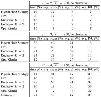
K = 2, |R| = 250, no clustering time (%) avg. nodes (%) avg. el. (%) avg. R/U (%)

Pigeon Hole Strategy 16 12 3 7

01*0 20 17 3 9

Kucherov K + 1 13 7 4 7

Kucherov K + 2 15 8 2 9

Opt. Kianfar 15 7 4 7

01*0 28 48 31 15

Kucherov K + 1 21 23 29 13

Kucherov K + 2 21 22 13 14

01*0 45 99 62 40

Kucherov K + 1 29 50 47 34

Kucherov K + 2 26 44 34 38

ManBest 24 48 27 35

TABLE III: Relative increase in workload without clustering when aligning of 100 000 reads of average length 250 bp to the human genome as compared to the figures in table I.

is around 1.1. In contrast, the speed-up from storing the bitvectors in an interleaved manner for the 01*0 search scheme and for K = 4 is around 1.7.

C.2.b Clustering. Clustering is a theoretical improvement that re-duces the search space. Clustering leads to fewer intermediate reports. For each intermediate report, a search is started, often for nodes close to each other in the search tree. This can lead to a large number of redundant computations. The higher the value for K, the bigger the impact of clustering as the maximal size of a cluster is 2K + 1. For K = 1, the impact is negligible. For higher values of K, the relative increase per metric is given in table III. It is clear that all strategies benefit from clustering. The Kianfar search scheme for K = 4 seems to benefit the least. This strategy had an average number of nodes and matrix elements that was already some magnitudes larger than the other strategies which explains why the relative increase is quite small.

An increase in the defined metrics does not automatically translate in the same increase in running time, as clustering also introduces some overhead. Nevertheless, the speed-up is often on par with the speed-up of interleaving the bitvectors, a purely implementation improvement.

Collectively, they prove that efficiently implementing a search scheme has a far higher impact than selecting the best search scheme. C.2.c Early Exact Matching. The results with and without early exact matching are compared for different values of K and search strategies are shown in table IV. It is clear that Kianfar’s scheme benefits the most from the early exact matching improvement, for K = 3 and especially for K = 4. This is due to the searches for which U[0] equals 1 and respectively 2. The search of the first piece is in the most dense region of the search tree, thus switching early to exact matching will greatly reduce the number of nodes visited and the accompanying matrix el-ements. However, all schemes benefit somewhat from this improve-ment. Especially the number of matrix elements reduces significantly with early exact matching. This effect is larger for larger values of K.

This improvement accelerates the approximate matching procedure, but has less effect than interleaving the bitvectors or clustering. C.3 Reusing Results of First Piece

The only search schemes that have at least two searches Siand Sj, for which πi[0] = πj[0], Ui[0] = Uj[0]and Li[0] = Lj[0], are the strategies by Kucherov. Kucherov K + 1 and K + 2, with K = 4,

K = 2, |R| = 250

no early exact matching early exact matching time avg.nodes avg. el. time avg. nodes avg. el.

P H. S. 11.0 s 479.53 1181.46 9.9 s 476.76 805.49 01*0 10.3 s 467.99 958.12 8.9 s 463.53 595.61 K. K + 1 9.9 s 428.16 872.90 8.9 s 425.92 536.30 K. K + 2 11.1 s 493.49 952.81 9.4 s 488.23 551.88 Opt. Kian. 9.7 s 416.75 817.91 8.7 s 414.55 498.52 K = 3, |R| = 250

no early exact matching early exact matching time avg.nodes avg. el. time avg. nodes avg. el. P H. S. 16.3 s 762.12 2791.06 14.2 s 753.66 2075.66 01*0 13.8 s 649.69 1859.66 11.9 s 640.43 1330.90 K. K + 1 11.7 s 517.99 1311.70 10.6 s 513.44 910.73 K. K + 2 11.7 s 543.92 1284.48 10.1 s 535.73 843.60 Opt. Kian 46.3 s 4028.99 12 116.84 26.6 s 1789.13 1436.86 K = 4, |R| = 250

no early exact matching early exact matching time avg.nodes avg. el. time avg. nodes avg. el. P. H. S. 26.3 s 1353.26 6389.06 22.3 s 1330.94 4950.71 01*0 19.3 s 988.31 3678.53 16.4 s 968.12 2826.91 K. K + 1 17.5 s 896.47 2888.98 14.9 s 882.04 2046.91 K. K + 2 18.6 s 1005.73 2857.85 15.4 s 981.93 1984.65 Opt. Kian. 13 m30 s 79 517.11395 568.36 5 m30 s 28 417.93 18 100.31 ManBest 17.6 s 830.92 2699.19 14.7s 808.48 1777.40

TABLE IV: Comparing the running time with and without early exact matching for different values of K and all search strategies. 100 000 reads of average length 250 bp were mapped to the human genome.

Kucherov K + 1 Kucherov K + 2 time avg. nodes time avg. nodes No reusing 16.0 s 990.22 17.6 s 1110.50 Reusing 14.9 s 882.04 15.4 s 981.93

TABLE V: Comparing the running times and visited number of nodes with and without reusing the results of the first piece for 100 000 reads of average length 250 and K = 4.

both have multiple groups of searches for which this kind of redun-dancy can be exploited. Specifically, for K = 2, Kucherov K + 2 has two searches for which the first piece and the first bounds are equal. As these search schemes only have searches that start with an exact search on the first piece, the only impact of this improvement will be on the number of nodes visited, since an exact search does not require an alignment matrix.

The results for the number of nodes and running time for these two strategies and K = 4 are given in table V. The number of nodes in-creases by more than 10% if one does not reuse the results of the first piece. Reusing the results of the first piece, thus has a positive ef-fect on the running time of these schemes, although the efef-fect is not as significant as interleaved bitvectors or clustering. Additionally, this improvement is only relevant for search schemes that suffer from this kind of redundancy.

D. Effect of Length of the Read

To study the effect of the length of the read has on the different search schemes, the 100 000 reads of length 100 were also aligned to the ref-erence genome.

For K ≤ 2, all search schemes perform better on shorter reads. The average number of nodes and matrix elements is smaller for shorter reads and small values of K. However, the average number of reported occurrences over unique occurrences increases for all schemes. As ex-pected, the number of unique occurrences is larger for shorter reads. Shorter reads have a higher probability, as compared to longer reads, of occurring in the text with less than K errors. An occurrence with less than K errors gives way to redundant occurrences, where characters 5

(12)

are deleted or inserted at the beginning or at the end of the occurrence. Clearly, if there are more unique occurrences, it is more likely that a redundant occurrence will be found as well.

For K = 3, only the search schemes by Kucherov et al. perform bet-ter for shorbet-ter reads. The scheme by Kianfar et al. and the backtracking schemes perform similar as on reads of average length 250. The pigeon hole strategy shows a sharp increase in nodes and matrix elements.

For K = 4, all schemes perform worse, although the schemes by Kucherov et al. are the least affected. This can be explained by the fact that reads of length 100 and up to 4 allowed errors will probably have more occurrences and more false leads than longer reads with the same number of allowed errors.

E. Space-Time Tradeoff

An increase in redundant reports means that more redundant accesses to the suffix array are required. If the suffix array is stored with a sparseness factor of 1, it is likely that this entry is cached and that the redundant report will not affect the running time much. However, if the sparseness is greater it is possible that this entry is not cached and needs to be recalculated. Redundant reports could then influence the running time. A higher sparseness factor will increase the running time for all search schemes.

Figure 2 shows the required memory for aligning reads to the human genome, and veryfiying the reported occurrences, as a function of the sparseness factor of the suffix array. Note that the required memory converges to 10 GB of memory.

For sparseness factors larger than 16, the memory improvement is negligible compared to the overall memory required. As high-end lap-tops currently have at least 16 GB of random access memory, it is clear that one could align on the human genome with a sparseness factor of only 4 using a laptop.

Fig. 2: Memory required for reading in a bidirectional FM-index and aligning 100 000 reads of length 250 on the human genome as a func-tion of the sparseness factor.

The running times for the different sparseness factors for all strate-gies and different values of K are shown in figure 3. The fluctuation of the running time due to the load of the machine is sometimes higher than the increase due to a higher sparseness factor. For sparseness fac-tors lower than 64, the effect on performance seems quite small. In order to compare the results more accurately, the experiments should be run on a bigger dataset and be repeated multiple times to get a mean and standard deviation.

F. Comparison with Seqan

To the best of our knowledge, SeqAn3 [16] is the only publicly avail-able library that implements search schemes to date. This implementa-tion is based on the optimal search schemes by Kianfar et al. [9].

This implementation was tested on the same dataset for reads of length 250. The running times are compared to the best running time

(a) K = 1 (b) K = 2

(c) K = 3 (d) K = 4

Fig. 3: Comparing the running times for the alignment of 100 000 reads of length 250 for all strategies on an FM-index with a different sparse-ness factor for different values of K.

K = 1 K = 2 K = 3 K = 4

Best 6.8 s 8.7 s 10.1 s 14.7 s

Opt. Kianfar 7.1 s 8.7 s 25.6 s 5 m30 s SeqAn v3.0.1 24.0 s 4 m48 s 2 h 25 m >1 d

TABLE VI: Comparing the performance of the best result of our im-plementation to the performance of Optimal Kianfar in our implemen-tation and to the performance of SeqAn3.

achieved by our implementation, as well as the running time of our implementation of the schemes by Kianfar et. al.

Table VI shows the results achieved by SeqAn3 as compared to our own implementation. Kianfar et al. performed the worst for higher val-ues of K in our implementation, but compared to the results of SeqAn3, this scheme still achieves reasonable results.

VII. CONCLUSION

The goal of this thesis was to analyze and improve the performance of lossless algorithms for approximate pattern matching. Such algo-rithms are guaranteed to retrieve all approximate matches of a pattern Pin a reference text T .

We demonstrated that the bidirectional FM-index is a succinct data structure that enables lossless approximate pattern matching on the hu-man reference genome with relatively modest memory requirements. The implementation makes use of the rank9 data structure, which sup-ports rank() operations in constant time. Aligning reads using the bidirectional FM-index to the human genome is feasible on a modern high-end laptop.

Search schemes organize the search procedure in such a way that un-successful branches in the search tree can be eliminated quickly. The new concept of clusters was introduced. By eliminating redundant in-termediate reports, the search space decreases significantly. In some cases the search space was halved.

We have shown that the rank9 data structure can be stored in memory in an interleaved manner for DNA sequences, which reduces the num-ber cache misses and thus positively impacts the running time. The gain in performance due to an improved implementation was found to be higher than changing to a more performant search scheme.

We also found that the “optimal” search schemes proposed by Kian-6

(13)

far et al. did not perform optimally for the edit distance metric and higher values of K. An in-depth comparison of several search schemes was provided for different metrics.

The research in this paper could be used to further accelerate lossless approximate matching, which can provide a new research direction for read mapping tools.

A. Future Work

The realized implementation can be improved further, both theoret-ically and implementation-wise. Below, we list some directions for further research.

The approximate pattern matching procedure that uses search schemes requires only read access to the bidirectional FM-index. For this reason, the search procedure can easily be parallelized using threads if multiple patterns need to be aligned.

Kucherov et al. noted that it might be more efficient to partition a search pattern into pieces of unequal length. For example, in the scheme with K = 4 and K + 1 pieces, the first search S0allows up to two errors in its second piece (U0[1] = 2) whereas the other searches Sionly allow a single error in their second piece (Ui[1] = 1). Hence, it can be beneficial to decrease the size of the piece π0[1] = 1. Kucherov et al. show in their paper that, within certain limits, enlarging the size of the piece π0[0]and decreasing the size of piece π0[1]leads to com-putational gain. So, one could, for each search scheme, calculate the theoretically optimal partitioning of the search pattern.

Another approach is to choose the partition sizes dynamically, de-pending on the contents of the pattern P itself. Most search schemes consist of searches that start with an exact match for their first piece. To balance the workload between searches, one could balance the size of the corresponding ranges for those pieces. In other words, one could try to choose the partition sizes in such a way that each piece roughly has the same number of exact occurrences.

In our own experiments, we noticed that the sizes of the ranges of the exact matches for search schemes with K = 4 ranged between 1 and 23 281for reads of length 250 and between 1 and 994 505 for reads of length 100, a difference of almost six orders of magnitude. These values were found for search schemes that partition the pattern into K+ 2pieces, as is to be expected as these pieces will be shorter. However, the other search schemes, with K + 1 pieces, still reported a maximum value as high as 555 168. We expect that a dynamic partitioning of the search pattern P can better balance these differences in workload.

There is a large variability in workload between patterns, depending on the presence or absence of substrings in P that are highly repetitive in T . For example, the number of nodes visited in the search tree to align a pattern, with K = 4 and the ManBeststrategy ranges between 308and 224 070 – a difference of three orders of magnitude. In other words, certain patterns are computationally cheap to align, whereas oth-ers require the exploration of a very large search space.

Even though ManBestperforms the best on average, it is not the best scheme in all scenarios (see table VII). As most search schemes parti-tion the pattern either in K + 1 or K + 2 pieces, and if the partiparti-tioning is the same for all search schemes it might be beneficial to calculate the exact ranges of each piece (which is a relatively cheap operation) and leverage this information (the size of the ranges and thus the sizes of the underlying subtrees) to dynamically select an appropriate search scheme.

During the search procedure it is not uncommon to visit a node of which the range has size 1. Even more, often this range is already achieved after the exact search of the first piece. It might be more beneficial to, instead of accessing the FM-index datas tructure, align the remaining pattern directly to T . The remaining piece of P is then aligned directly to the substring of T that follows (or precedes) the oc-currence using a bit-parallel algorithm [17, 18] and the remaining edit distance. The Bwolo tool by Vroland et al. [14], makes use of 01*0 seeds, a unidirectional FM-Index and in-text verification. This tool

of-|R| = 250 |R| = 100

min(nodes) max(nodes) min(nodes) max(nodes)

Pigeon H. S. 315 430 162 162 1 147 116 01*0 315 336 887 159 815 858 Kuch. K + 1 309 388 469 156 702 932 Kuch. K + 2 358 209 712 174 387 023 Opt. Kianfar 15 663 335 075 14 964 589 586 ManBest 308 224 070 155 428 697

TABLE VII: Minimum and maximum values for the number of nodes visited for each scheme during the alignment of one pattern with aver-age length |R| and K = 4.

ten achieves better results than full-fleshed search schemes. Pockrandt acknowledged this in his PhD dissertation and found that for Hamming distance a speedup of 1.6 to 2.1 can be achieved if one switches to in-text verification if the number of occurrences is 25 or lower [12].

For all search schemes, for which the searches start with an error-free piece, the increase in running time between K = 3 and K = 4 is only 50% for reads with average length 250 (see table I). For this reason, the performance of search schemes for the alignment with more errors might be reasonable and is worthwhile to be researched. Such search schemes might be beneficial for sequencing technologies that produce reads with a high error rate, such as Pacific Biosciences or Oxford Nanopore platforms.

REFERENCES

[1] J. L. Peterson, “Computer programs for detecting and correcting spelling errors,” Communications of the ACM, vol. 23, no. 12, pp. 676–687, 1980.

[2] F. Sanger and H. Tuppy, “The amino-acid sequence in the phenylalanyl chain of insulin. 1. the iden-tification of lower peptides from partial hydrolysates,” Biochemical Journal, vol. 49, no. 4, p. 463, 1951.

[3] ”National Human Genome Research Institute (NHGRI)”, “Dna sequencing costs: Data.” https://www.genome.gov/about-genomics/fact-sheets/ DNA-Sequencing-Costs-Data. Accessed: 2020-05-18.

[4] P. Ferragina and G. Manzini, “Opportunistic data structures with applications,” in Proceedings 41st Annual Symposium on Foundations of Computer Science, pp. 390–398, IEEE, 2000.

[5] T. W. Lam, R. Li, A. Tam, S. Wong, E. Wu, and S.-M. Yiu, “High throughput short read alignment via bi-directional bwt,” in 2009 IEEE International Conference on Bioinformatics and Biomedicine, pp. 31–36, IEEE, 2009.

[6] G. Kucherov and D. Tsur, “Approximate string matching using a bidirectional index,” CoRR, vol. abs/1310.1440, 2013.

[7] M. Burrows and D. Wheeler, “A block-sorting lossless data compression algorithm,” in DIGITAL SRC RESEARCH REPORT, Citeseer, 1994.

[8] S. Vigna, “Broadword implementation of rank/select queries,” in International Workshop on Exper-imental and Efficient Algorithms, pp. 154–168, Springer, 2008.

[9] K. Kianfar, C. Pockrandt, B. Torkamandi, H. Luo, and K. Reinert, “FAMOUS: fast approximate string matching using optimum search schemes,” CoRR, vol. abs/1711.02035, 2017.

[10] G. A. Pavlopoulos, A. Oulas, E. Iacucci, A. Sifrim, Y. Moreau, R. Schneider, J. Aerts, and I. Iliopou-los, “Unraveling genomic variation from next generation sequencing data,” BioData mining, vol. 6, no. 1, p. 13, 2013.

[11] X. Yang, S. P. Chockalingam, and S. Aluru, “A survey of error-correction methods for next-generation sequencing,” Briefings in bioinformatics, vol. 14, no. 1, pp. 56–66, 2013.

[12] C. M. Pockrandt, Approximate String Matching: Improving Data Structures and Algorithms. PhD thesis, Freie Universit¨at Berlin, 2019.

[13] P. Fletcher and C. W. Patty, Foundations of higher mathematics /. Boston :: PWS-Kent Pub.,, 2nd ed. ed., 1992.

[14] C. Vroland, M. Salson, S. Bini, and H. Touzet, “Approximate search of short patterns with high error rates using the 01∗ 0 lossless seeds,” Journal of Discrete Algorithms, vol. 37, pp. 3–16, 2016. [15] V. A. Schneider, T. Graves-Lindsay, K. Howe, N. Bouk, H.-C. Chen, P. A. Kitts, T. D. Murphy,

K. D. Pruitt, F. Thibaud-Nissen, D. Albracht, R. S. Fulton, M. Kremitzki, V. Magrini, C. Markovic, S. McGrath, K. M. Steinberg, K. Auger, W. Chow, J. Collins, G. Harden, T. Hubbard, S. Pelan, J. T. Simpson, G. Threadgold, J. Torrance, J. Wood, L. Clarke, S. Koren, M. Boitano, H. Li, C.-S. Chin, A. M. Phillippy, R. Durbin, R. K. Wilson, P. Flicek, and D. M. Church, “Evaluation of grch38 and de novo haploid genome assemblies demonstrates the enduring quality of the reference assembly,” bioRxiv, 2016.

[16] K. Reinert, T. H. Dadi, M. Ehrhardt, H. Hauswedell, S. Mehringer, R. Rahn, J. Kim, C. Pockrandt, J. Winkler, E. Siragusa, G. Urgese, and D. Weese, “The seqan c++ template library for efficient sequence analysis: A resource for programmers,” Journal of Biotechnology, vol. 261, pp. 157 – 168, 2017. Bioinformatics Solutions for Big Data Analysis in Life Sciences presented by the German Network for Bioinformatics Infrastructure.

[17] J. Loving, Y. Hernandez, and G. Benson, “BitPAl: a bit-parallel, general integer-scoring sequence alignment algorithm,” Bioinformatics, vol. 30, pp. 3166–3173, 07 2014.

[18] G. Myers, “A fast bit-vector algorithm for approximate string matching based on dynamic program-ming,” Journal of the ACM (JACM), vol. 46, no. 3, pp. 395–415, 1999.

(14)

List of Symbols And Abbreviations XI

List of Symbols And Abbreviations

$ Sentinel character.

A(X, Y ) Alignment of two sequences X and Y .

Σ Alphabet.

AM Alignment Matrix.

BVc rank9 bitvector for character c.

C The counts array of an FM-index. ED(X, Y ) Edit distance between strings X and Y .

HD(X, Y ) Hamming distance between two strings X and Y . INi,j(S) Infix.

Occ The occurrences table of an FM-index. PREj(S) Prefix.

SUFi(S) Suffix.

BWT Burrows-Wheeler Transformation.

DNA Deoxyribonucleic acid.

HTS High-Throughput Sequencing.

NUMA Non-uniform Memory Access.

RAM Random-access memory.

SA Suffix Array.

(15)

1 |

Introduction

Approximate string matching is a well-studied problem in computer science. Commercial spell checkers have been around since the 1970s [1]. After Frederick Sanger determined the se-quence of insulin in the early 1950s [2] and protein sese-quences became available, the need for automated sequence alignment in molecular biology arose and sequence alignment algorithms became central to bioinformatics applications.

In 1977, the DNA of a phage was sequenced [3]. Since then, sequencing costs have decreased dramatically and the genomes of thousands of organisms have been determined. With the advent of High-Throughput Sequencing (HTS) methods (low-cost and highly parallelizable se-quencing), the accumulated data grows faster and faster. The Sequence Read Archive (SRA) is a large sequence database led by an international organization, which stores data from HTS experiments. Figure 1.1 compares the data growth of the SRA to the number of transistors in a CPU. Moore’s law is the observation that the number of transistors in an integrated circuit dou-bles every 1.5 to 2 years along with a similar increase in a CPU’s compute power [4]. Clearly, the advancements in computer architecture are insufficient to keep up with the ever growing database of sequences.

Figure 1.1: The number of megabases sequenced in the SRA compared to the transistor count on a logarithmic scale [5].

In 2003, the human genome project was completed and for the first time, the DNA sequence of a human individual was established. This project took 13 years and cost over 3 billion USD.

(18)

INTRODUCTION 2

Today, the genome of any human can be sequenced for under a 1000 USD (see figure 1.2). HTS methods allow for cheap and parallel sequencing of DNA, however, they fragment the DNA into millions of reads with no information on how they fit together. Among many other applications, this is where approximate pattern matching comes into play.

Figure 1.2: Comparing the cost per human genome to Moore’s Law [6].

Formally, given a query pattern P (e.g. a read) and a search text T (e.g. a reference genome or a database of genomes), the basic task is to identify occurrences of P in T . If no errors are allowed, the problem is called exact pattern matching. Due to the presence of sequencing errors and natural variation (human individuals share roughly 99.9% of their DNA), one is often interested in finding occurrences of P in T within a certain Hamming distance (allowing only sub-stitutions) or Levenshtein/edit distance (allowing substitutions, insertions and deletions). This is called approximate pattern matching. As most practical bioinformatics applications perform many queries for a given static search text T , the focus of this thesis is on approximate pattern matching using a full-text index.

Most bioinformatics tools (e.g. BLAT, BLAST, BWA, etc.) use lossy approximate pattern match-ing algorithms: they rely on heuristics to quickly identify some (but not necessarily all) approx-imate matches of P in T . By sacrificing some sensitivity, significant gains in performance can be obtained. This loss of sensitivity can manifest itself in many ways, for example, reads can be over-confidently mapped to the wrong position in genome, causing false-positive germline or somatic variants to be called. In contrast, in this thesis, the focus is on lossless algorithms that are guaranteed to retrieve all approximate matches of P in T .

Many approximate string matching techniques that exist for normal text, like inverted files, string B-trees and prefix indexes, are not suitable for bioinformatics applications because biological sequences cannot be broken up into words [7]. However, some techniques, like suffix trees and suffix arrays were applicable with good results [8]. In 2000, a new substring index, the FM-index, was proposed [9]. This index still allows for the alignment of sequences to a reference

(19)

INTRODUCTION 3

text in linear time of the pattern’s length, while having the benefit of being a very succinct (i.e. memory-friendly) data structure. In 2009, Lam et al. extended the unidirectional FM-index to a bidirectional FM-index. Using a bidirectional FM-index, patterns can be matched either from left to right, or from right to left. Curiously, this additional functionality opens up new possibilities for faster approximate matching [10]. Chapter 3 discusses and analyzes both the unidirectional and bidirectional FM-index.

The naive algorithm for approximate pattern matching (called ‘backtracking’) is discussed in chapter 4. In this thesis, the inherent redundancy associated with edit distance alignments is analyzed and an improved version of the naive algorithm is proposed.

In 2015, Kucherov et al. introduced the concept of search schemes. Informally, search schemes define how a pattern P is matched using a bidirectional index such that unsuccessful branches of the search tree are discarded as quickly as possible and runtime is minimized [11]. This concept is discussed in chapter 5.

Chapter 6 describes a number of improvements on the approximate pattern matching problem using the bidirectional FM-index, of which all but one are new concepts.

In chapter 7, the performance of different search schemes is assessed. Additionally, the effects of the new improvements in chapter 6 are investigated, as well as the effect of read length and the space-memory trade-off. Finally, chapter 8.1 identifies some directions for future work. The goal of this thesis is to analyze and improve the performance of lossless algorithms, like search schemes, that are guaranteed to retrieve all approximate matches of a pattern P in a reference text T .

(20)

DEFINITIONS AND NOTATION 4

2 |

Definitions and Notation

First, some formal definitions and notations used throughout this thesis are introduced.

Definition 2.0.1. — StringA string is a finite sequence of characters over the alphabet Σ. The

length of a string S is denoted by |S|. The reverse of string S is denoted as S0_.

Remark. Here, as in most programming languages, strings are indexed starting from zero.

Definition 2.0.2. — Empty stringThe empty string is a string of length 0. The empty string is

written as "".

Definition 2.0.3. — Alphabet (Σ)The alphabet Σ over a string S is the set of unique characters in the string.

Definition 2.0.4. — Range A range is a pair of integers i and j, with i ≤ j, that defines a

half-open interval [i, j). The size of the range is j − i. Note that [i, i) denotes the empty range. A range S[i, j) over a string S corresponds to all characters S[k], with 0 ≤ i ≤ k < j ≤ |S|. Ranges over arrays can be defined analogously.

Remark. The end of a range is non-inclusive. As a result, S[0, |S|)= S, and thus the end of S corresponds to |S|. This, together with the starting of indexing at zero is the convention preferred by Dijkstra [12] and is also adopted by the ISO C++ standard [13].

Definition 2.0.5. — Infix, Suffix and Prefix An infix INi,j(S)of S is a substring of S,

corre-sponding to S[i, j). A suffix SUFi(S)of S is a special kind of infix where the end of the infix is

the end of S (=INi,|S|(S)). Analogously, a prefix PREj(S)is an infix where the beginning is the

beginning of S (=IN0,j(S)).

Example 2.0.1. Assume S = "abcdef". Then, S[0] = ‘a’, S[1] = ‘b’, S[2] =‘c’, . . . The suffix

SUF3(S)is "def", PRE5(S)equals "abcde" and the infix IN2,5(S)equals "cde".

Definition 2.0.6. — (Substring) index A substring index is a data structure in which a

pre-processed static text is stored. It allows for querying the text for matches of substrings with a sublinear time complexity.

Definition 2.0.7. — Forward and backward search In most indexes, query strings are

searched character by character, either from left to right or from right to left. A forward search of a pattern P starts its search with the prefix PRE1(P ) and extends this prefix character by

character to the right, until PRE|P |(P )= P is matched or no match could be found. Likewise, a

backward search starts with the suffix SUF|P |−1(P )and extends this suffix character by

(21)

DEFINITIONS AND NOTATION 5

Definition 2.0.8. — Unidirectional index A unidirectional index is an index that either only

supports backward or forward searching.

Definition 2.0.9. — Bidirectional index A bidirectional index is an index that supports both

forward and backward searching.

Definition 2.0.10. — Sentinel character ($)In order to lexicographically compare two strings

of different length, a sentinel character, denoted as $ /∈ Σ is appended to each string. It is defined as either larger or smaller than any character in Σ. In this dissertation, the sentinel character is always the smallest character. The sentinel character is appended to the end of a string and does not occur anywhere else in this string. For notation purposes, it is assumed that all strings S over an alphabet Σ already have the sentinel character appended and therefore S[|S| − 1] = $. The sentinel character will also be used to uniquely define an ordering of cyclically rotated strings, see section 3.

Definition 2.0.11. — Lexicographical orderingThe lexicographical ordering of two strings X

and Y of equal length n is defined as:

X <LexY ⇐⇒ ∃i ∈[0, n) : ∀j < i : X[j] = Y [j] ∧ X[i] < Y [i] (2.1)

The ordering of two strings X and Y , where Y is shorter than X, is found by padding Y with the sentinel character until the two strings are of equal length and then applying formula 2.1 to X and the padded Y string. Analogously, if X is shorter than Y , then X is padded and the formula is applied to the padded X and Y string. ≤Lexcan be defined analogously, from which

=Lex, ≥Lex and >Lex can be easily derived. The alphabetical ordering used in conventional

dictionaries corresponds to this ordering.

Additionally, the ordering of two strings X and Y up to m characters can be defined. This ordering only considers the first m characters and is defined as:

X <Lex,m Y ⇐⇒ X[0, min(|X|, m)) <LexY[0, min(|Y |, m)) (2.2)

(22)

FM-INDEX 6

3 |

FM-index

The FM-index a substring index proposed by Ferragina and Manzini in 2000 [9]. It is based on the Burrows-Wheeler Transformation (BWT) [14].

3.1 BWT

The BWT is a reversible transformation that rearranges a text into a new text that contains the same characters as the original one. The result of this transformation is denoted as BWT(S) and is again a string. This transformation has the tendency to cluster equal characters together, making it easier to compress the transformed string.

The BWT(S) is constructed by lexicographically sorting all cyclic rotations of S and extracting the last character of each rotation. This algorithm is described in algorithm 1 and makes use of two helper functions: one that cyclically rotates a string S by a number of characters and one that lexicographically sorts an array of strings.

Algorithm 1:Burrows-Wheeler Transformation Input :String S of n characters

Output:String BW T , the transformation of S

1 cyclicRotations ←[] 2 for i ←0 to n − 1 do 3 cyclicRotations.add(S.rotate(i)) 4 end 5 sortedRotations ←sortLexicographically(cyclicRotations) 6 BW T ←“” 7 for i ←0 to n − 1 do 8 BW T.add(sortedRotations[i][n − 1]) 9 end

Remark. The lexicographically ordered array of cyclic rotations of a string S with length n can be seen as an n × n matrix M, where the last column corresponds to BWT(S).

Remark. Since the rows of matrix M all correspond to a unique cyclic rotation of string S, all columns of matrix M are a permutation of string S. The first column of this matrix M is the permutation of S where the characters are lexicographically sorted.

Example 3.1.1. Consider the string S = “banana$” of length 7. The transformation is illustrated

(23)

3.1 BWT 7

ordering of these rotations. The BWT(S) is the sequence of final characters, indicated in color and underlined. Thus, BWT(S) = “annb$aa”.

banana$ $banana

anana$b a$banan

nana$ba sort ana$ban

ana$ban ⇒ anana$b

na$bana lexicographically banana$

a$banan na$bana

$banana nana$ba

Remark. As stated in definition 2.0.10, the sentinel character is always the lexicographically smallest character. It effectively acts as a tiebreaker when sorting the rotations.

Another way to construct BWT(S) is via the Suffix Array (SA) of the string.

Definition 3.1.1. — Suffix Array (SA)A suffix array of a string S is a lexicographically sorted

array of all suffixes SUFi(S), with 0 ≤ i < |S|, it is denoted as SA(S). Only the subscripts i

of the suffixes SUFi(S)are stored along with string S instead of the actual suffixes, in order to

save space.

Remark. Note that due to the presence of the sentinel character, the sorted order of the suffixes of S corresponds to the sorted order of the rotations of S. Hence, the character at position i in BWT(S)is the character that immediately precedes SUFj(S), with j = SA(S)[i].

Formally: BWT(S)[i] =    S[SA(S)[i]] − 1] if SA(S)[i] > 0 $ otherwise (3.1)

Example 3.1.3 illustrates the relation between BWT(S) and SA(S).

LF Mapping

Definition 3.1.2. — LF PropertyConsider the matrix M that holds the lexicographically sorted

cyclic rotations of the string S. The ith occurrence of character c in the last column of M and the ith occurrence of c in the first column of M correspond to the same character in S.

To showcase the LF property, example 3.1.1 is revisited. This time, the characters are ranked as to distinguish occurrences of the same character.

Example 3.1.2. Consider the string “b0a0n0a1n1a2$0” of length 7 of example 3.1.1. The matrix

of sorted cyclic rotations is given below. One can see that the first occurrence of the character ‘a’ is a2in both the F and L column. The second occurrence is a1and third is a0. The order of

(24)

3.1 BWT 8 F L $0 b0 a0 n0 a1 n1 a2 a2 $0 b0 a0 n0 a1 n1 a1 n1 a2 $0 b0 a0 n0 a0 n0 a1 n1 a2 $0 b0 b0 a0 n0 a1 n1 a2 $0 n1 a2 $0 b0 a0 n0 a1 n0 a1 n1 a2 $0 b0 a0

The reason why the LF property holds is that both the characters in the F and in the L column are sorted by their right-context. This is due to the definition of lexicographical sorting and the cyclic nature of the rotations. For example in example 3.1.2, the right-contexts of a0, a1 and a2

are respectively “nana$”, “na$” and “$”.

The LF property can be used to map the index of a character c in the L column to the index of character c in the F column.

Example 3.1.3. Consider S = “banana$”. The F column, SA(S) and BWT(S) are given in

Table 3.1, as well as the suffixes corresponding to the entries of the suffix array. Applying equation 3.1 for i = 3 then gives: BWT(S)[3] = S[SA(S)[3] − 1] = S[1 − 1] = ‘b’. Note that F[k] = SUF_SA(S)[k](S)[0].

index SA(S) F BWT(S)= L SUF_SA(S)[index](S)

0 6 $ a $ 1 5 a n a$ 2 3 a n ana$ 3 1 a b anana$ 4 0 b $ banana$ 5 4 n a na$ 6 2 n a nana$

Table 3.1: SA(S), F column and BWT(S) for S = “banana$”.

3.1.1 Reversibility

The BWT is a reversible transformation. Using only the L and F column, and the LF property, it is easy to reconstruct the original string S. The F column can be derived from the L column by sorting the characters of L.

Reversing the BWT is easy once the following observation is taken into account.

Observation The character at the ith index position of L is the character that precedes the